A WORK PROJECT, PRESENTED AS PART OF THE REQUIREMENTS FOR THE AWARD OF A MASTER’S DEGREE IN ECONOMICS FROM THE NOVA SCHOOL OF BUSINESS AND
ECONOMICS
Non-linearities in Fiscal
Multipliers in EU15: A Panel
Data Threshold Model
Carlos Guilherme de Melo Gouveia
Student No. 868
A project carried on the Master’s in Economics Program under the supervision of:
Professor Paulo M. M. Rodrigues
Lisbon, 6
thJanuary 2017
1
1.
Introduction
Europe has suffered considerably from the collateral effects of the financial crisis of
2008, especially due to the sovereign debt crisis which was a side effect of the
previously mentioned crisis because of the increase in investor’s risk perception. This
last crisis affected many European countries, namely Greece, Portugal and Ireland that
needed bailouts to return to the markets.
Meanwhile, governments tried to reduce their expenses and increase their
revenues by reducing services and increasing taxes in those countries. The expected
effects were, of course, contractionary but countries felt that the consolidation of
public accounts were more important than making GDP return to its normal level in
the short run and giving those countries more favorable conditions in the future to
achieve their potential GDP.
This line of thought was instigated by the high interest rates that those countries
had to pay to have access to funds in the markets because investors felt that these
countries would not be able to repay their debt at those levels. So, states tried to show
that they were doing an enormous effort to make things right.
Nevertheless, the effects of the so called austerity measures were not as
anticipated and the contractionary effects were even larger than excepted. For
instance, Greece drowned into a spiral of impoverishment and its GDP lost more than
100 billion dollars in solely five years, which represents a drop of more than 30% while
its public debt level to GDP never stopped increasing. Portugal suffered massively, too,
but the Portuguese government was more successful in implementing those measures
and GDP is growing at modest rates since 2013.
The purpose of this study is to show that the effects were not as planned because
multipliers are not fixed and change when the economic conditions change. What we
will try to prove is that it is wrong to use multipliers obtained in regular periods when
you are facing an atypical event such as a crisis.
To do so, we will use the 15 countries that composed the European Union (EU)
from 2000 until 2016 (Austria, Belgium, Denmark, Finland, France, Germany, Greece,
Ireland, Italy, Luxembourg, the Netherlands, Portugal, Spain, Sweden and the United
Kingdom), and we will set up a Panel data regression threshold model, in order to
show that an increase in government expenditures has different impacts on GDP
2
This paper is organized as follows. Section 2 presents a literature review. Section 3
introduces the model we will use. Section 4 describes the data. Section 5 presents our
empirical results. Section 6 provides some robustness tests, and Section 7 puts forward
the conclusions.
2.
Literature Review
As a consequence of the crisis and the effects of policies with underestimated
results the subject of varying fiscal multipliers has started to arise and economists
restarted to see fiscal policy as a matter of study.
Even so, there are not many studies that look at fiscal multipliers in the way
that we are proposing in this work project as most of them use structural VAR
methodologies or just a narrative approach.
Structural VAR studies use recursive identification (Galí et al., 2007) or
extremely complex structures (Blanchard and Perotti, 2002). The first approach obtains
an instant multiplier of 0.8 and two years after a response of 1.8, whereas, the second
finds a peak spending multiplier between 0.9 and 2 depending on some assumptions
that the authors made.
In the narrative approach, authors look at newspapers or government reports
in order to get external information that may help them identify exogenous fiscal
shocks. Romer and Romer (2010) and Ramey (2011b) were some of the authors that
used this approach. Usually they find multipliers from 0.6 to 1.2 depending on the
sample and the underlying assumptions made.
However, since the Great Recession and the Sovereign Debt Crisis, economists
started to argue that fiscal multipliers may behave in a non-linear way depending on
the state of the economy. Almunia et al. (2010) and DeLong and Summers (2012)
showed that during the early 1930s (Great Depression) fiscal multipliers were larger
and Corsetti et al. (2012) used dummy variables to show that fiscal multipliers increase
during financial crisis.
To study this, we can use dummy variables, as Corsetti et al. have done, but we
think that using a threshold and allowing the model decide when the economy is in
one state or the other could eventually be more reliable.
Some economists thought in the same way and used a method similar to ours
3
Bachmann and Sims, 2012; Candelon and Lieb, 2013, Nunes and Poirier, 2014). Other
authors on the other hand used other variables in other to capture these states (see
e.g. Afonso et al., 2011; Baum et al., 2012a; and Ferraresi et al., 2014).
Nonetheless, our work is somehow different because it looks at the global EU15
and uses a panel data threshold model to reinforce that idea. This type of models was
first introduced by Hansen (1999, 2000) and to the best of our knowledge there has
been no application of this method to this particular subject. Chang et al. (2009)
applied it to the relationship between tourism specialization and economic
development and Kremer et al. (2012) used it to analyze the connection between
inflation and growth.
Our goal is to show that fiscal multipliers change conditionally on the output
gap, but using different samples of countries during several quarters. Our focus will be
the fifteen countries that were part of the European Union in the early 2000s.
3.
The Model
The model we used is an extension of the approach introduced by Hansen
(1999) which was developed by Kremer, Bick and Nautz (2012). Since we used their
model, we will explain it in an extremely similar way as they did.
This model allows the original setup to have endogenous regressors. Hence, we
will use GDP growth as our dependent variable and Investment growth as our
endogenous regressor, due to the Accelerator Theory that shows that investment
variations are highly correlated with variations in the output.
The model of interest can be written as:
( ) ( ) ,
where i = 1,…, 15 represents the first 15 countries joining the European Union by
alphabetical order and t=1,…, 62 is the time index. is the country-specific fixed effect. The error term is i.i.d. with mean 0 and variance σ2. I(.) is the function that
indicates the regime, and which is defined by the threshold variable, corresponds
to the output gap, and is the threshold level. is a vector of explanatory variables
which may include lagged values of the dependent variable, as well as exogenous and
4
3.1. Fixed-effects elimination
We start the estimation process by removing the fixed effects, , through a
fixed-effects transformation. To do so, we have to eliminate the country-specific fixed
effects without going against the distributional assumptions underlying Hansen (1999)
and Caner and Hansen (2004).
In this dynamic model, the transformation proposed by Hansen (1999) leads to
inconsistency because the lagged variable is always correlated with the transformed
individual errors. Hence, to overcome this problem, Kremer et al. (2012) used the
forward orthogonal deviations transformation proposed by Arellano and Bover (1995)
to eliminate the fixed effects. This transformation is especially virtuous because it
avoids serial correlation of the transformed error terms.
This transformation is not a simple first difference or the subtraction of the
mean from each observation. In this process the average of all future available
observations of a variable is considered.
The transformation is given by:
√ ( ( ) ],
where T is the total number of observations, (T=62 in our case).
Looking at the variance of the error terms, we observe that the error terms are
uncorrelated:
( ) ( ) .
3.2. Estimation
Following Caner and Hansen (2004), we then estimate a reduced form
regression for the endogenous variables as a function of the instruments and replace
them by their predicted values. In the second step, the main equation presented
before is estimated by least squares for a specific threshold value .
The threshold value is estimated by minimizing the sum of squared residuals.
The second step is repeated for a strict subset of the support of the threshold variable
and is fixed as the one that has the smallest sum of squared residuals. Standard
5
4.
Data
As previously indicated, this paper focuses on the 15 countries that constituted
the EU from 1995 until 2004, they are Austria, Belgium, Denmark, Finland, France,
Germany, Greece, Ireland, Italy, Luxembourg, the Netherlands, Portugal, Spain,
Sweden and the United Kingdom.
The variables used are GDP, Government Expenditures, Inflation and Output
Gap. GDP and government expenditures were obtained from Eurostat, GDP at market
prices and final consumption expenditure of general government were the items
chosen, both at current prices and seasonally and calendar adjusted. Inflation was
obtained from the OECD and Output Gap was obtained from the IMF for some
countries and from the OECD for others.
To avoid scale problems, GDP and Government Expenditures were used in per
capita values. To do so, we looked for Total Population in Eurostat and computed the
ratio.
All data is quarterly and refers to the period between 2000Q1 and 2016Q2. The
starting point was chosen because of data limitations for some countries which did not
report quarterly data until the beginning of the 2000s.
To compute inflation and output gap, we used a GDP weighted average. During
that time, the mean quarterly GDP of those 15 countries was 2859 billion euros, the
mean quarterly inflation was 0.43% and the economies spent more time with a
negative output gap than with a positive one, as 516 observations reveal an output gap
below zero.
5.
Empirical Results
To get the answers that we are looking for, we apply the panel threshold model
to our data in order to see if fiscal policy has different effects on GDP.
As mentioned before, our model consists of GDP as the dependent variable and
Government Expenses, Investment, Private Consumption, Real Exchange Rate,
Population, Prices and Lagged GDP as explanatory ones. All these variables are
expressed in growth terms. Output Gap is the variable that makes the model change
6
Investment growth is considered as endogenous due to the accelerator effect
proposed by Jorgenson (1963) which says that variations in investment are highly
correlated with variations in GDP growth.
As instruments, we use lags of the endogenous variable: investment growth. In
our application we just used one lag.
5.1. Threshold selection
The first step to get our results is to endogenously select the threshold value
that shifts our model from one regime to another. We decided to use just one
threshold that minimizes the sum of squared residuals as clarified before.
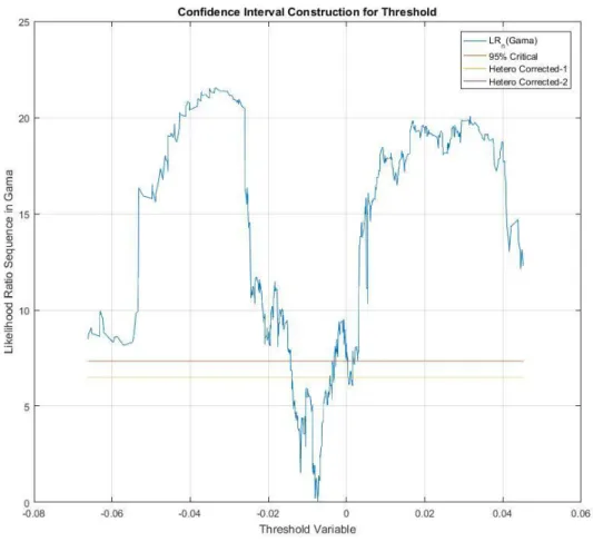
Figure 1 - Threshold selection
As can be observed from figure 1, our model provides the result that the value
of the output gap that makes the economy shift from one regime to another is
-0.7307%.
The 95% confidence interval is between -1.4303% and 0.1527%. This shows that
when the output gap gets slightly negative or zero, the economy changes its behavior
7
5.2. Slopes and Standard Errors
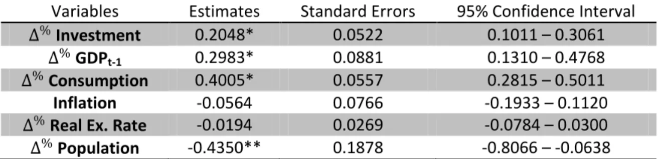
For the variables which do not depend on the regimes we observe that all
variables, with the exception of Inflation and Real Exchange Rate change, are
significant. 1
Variables Estimates Standard Errors 95% Confidence Interval
Investment 0.2048* 0.0522 0.1011 – 0.3061
GDPt-1 0.2983* 0.0881 0.1310 – 0.4768
Consumption 0.4005* 0.0557 0.2815 – 0.5011
Inflation -0.0564 0.0766 -0.1933 – 0.1120
Real Ex. Rate -0.0194 0.0269 -0.0784 – 0.0300
Population -0.4350** 0.1878 -0.8066 – -0.0638
Table 1 - Regime Independent Variable
Regarding Government Expenses, we found that its behavior is only significant
when the output gap is negative. This reinforces the idea that governments must
intervene when the economy is facing negative output gaps and that interventions
when the economy is overheated are pointless.
Government Expenses Estimates Standard Errors 95% Confidence Interval
Output Gap < -0.7307% 0.1021* 0.0342 0.0429 – 0.1778
Output Gap > -0.7307% 0.0357 0.0331 -0.0067 – 0.1253
Table 2 - Regime Dependent Variable
This model also allows for a constant term whenever the threshold variable is
below the threshold value, so, whenever we are facing an output gap below -0.007307,
the economy tends to grow, but at low levels.
Constant Term Estimate Standard Error 95% Confidence Interval
Output Gap < -0.7307% 0.0011* 0.0005 0.0005 – 0.0026
Table 3 – Regime Specific Constant Term
These results confirm that fiscal policy is an important tool whenever
economies are in recession.
In order to confirm our findings, we also performed some robustness tests by
changing the countries selected and the time frame that we are analyzing.
6.
Robustness Tests
In order to see if our conclusions hold under different circumstances, we
decided to performsome robustness checks by changing the data frame.
8
We will analyze the results of running the model without the “PIGS” countries
and the results of a model just with “PIGS” countries. Furthermore, we will also redo
the analysis by discarding the period after 2009 as well as looking only at the period
after 2009.
When trying to perform the model with GDP growth or lagged GDP growth as
threshold variable, the results showed that the threshold value is fixed for high levels
of growth, which is a problem because one regime ends up with extremely few
observations.
6.1. Without “PIGS”
During the years that we are considering, four countries received external aid.
Portugal, Ireland, Greece and Spain got through the crisis with even more difficulties
than the rest of the EU countries. In order to see if their removal from our sample
changes our conclusions significantly, we decided to redo the entire model with just 11
countries, i.e., without the so-called “PIGS”.
Threshold Value 95% Confidence Interval -0.7307% -1.1922% – -0.3751%
Table 4 - Threshold Value Without PIGS
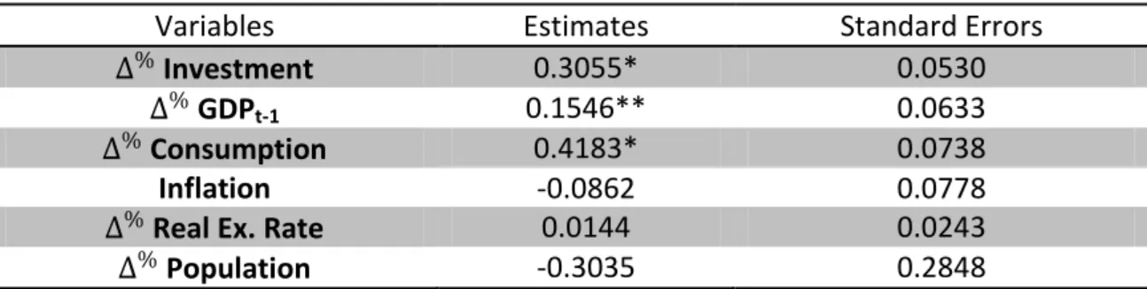
Variables Estimates Standard Errors
Investment 0.3055* 0.0530
GDPt-1 0.1546** 0.0633
Consumption 0.4183* 0.0738
Inflation -0.0862 0.0778
Real Ex. Rate 0.0144 0.0243
Population -0.3035 0.2848
Table 5 - Regime Independent Variables Without PIGS
Government Expenses Estimates Standard Errors
Output Gap < -0.7307% 0.1520* 0.0506
Output Gap > -0.7307% 0.0358** 0.0499
Table 6 - Regime Dependent Variable Without PIGS
Constant Term Estimate Standard Error
Output Gap < -0.7307% 0.0006** 0.0005
Table 7 - Regime Specific Constant Term Without PIGS
These results confirm our previous results and reinforce them, since we can see
that in the 11 countries that did not face external aid during the crisis, fiscal policy has
9
However, even though it is true that these results reinforce our previous
findings, it means that in PIGS, things are not so well behaved as in the other countries.
6.2. “PIGS”
In this restricted sample, the results go against our previous findings. However,
the fact that only Investment, Real Exchange Rate and Government Expenses in
periods in which the output gap is above the threshold value are significant, reinforces
the idea that these countries should be seen as outliers.
Threshold Value 95% Confidence Interval -3.0733% -8.6247% – -2.9149%
Table 8 - Threshold Value for PIGS
Variables Estimates Standard Errors
Investment 0.2359** 0.1030
GDPt-1 0.3246*** 0.1817
Consumption 0.1480 0.1300
Inflation 0.1505 0.2007
Real Ex. Rate -0.2415** 0.0973
Population -0.9096** 0.4007
Table 9 - Regime Independent Variables for PIGS
Government Expenses Estimates Standard Errors
Output Gap < -3.0733% 0.0055 0.0559
Output Gap > -3.0733% 0.0914** 0.0478
Table 10 - Regime Dependent Variable for PIGS
Constant Term Estimate Standard Error
Output Gap < -3.0733% -0.0047** 0.0020
Table 11 - Regime Specific Constant Term for PIGS
Even though it seems that the results go against the previous ones, we have to
look carefully at this output. Firstly, we can see that the standard errors increased in
every variable which shows that these countries went through agitated moments
which increased the uncertainty of the parameters a lot.
Also, this model presents a very low threshold value that is only observable
after the sovereign debt crisis in these four countries, and, so, it is important to
understand that one regime is purely showing us results from the crisis whereas the
other is just allowing us to understand what happened before it.
Furthermore, we cannot forget that economies have a tendency to go to
equilibrium and that equilibrium is when the output gap is close to zero, so, although
10
go to equilibrium, i.e., to grow. This explains why when governments were diminishing
their expenses, GDP did not fall as much as was expected.
In sum, this model in this subsamble demonstrates a lot of uncertainty
measured by the standard errors, has a low threshold value and the pressure of the
economy to go to equilibrium is quite high and contractionary measures have no great
contractionary effects.
6.3. No Crisis
The crisis that began in 2009 showed another side of the economy. A side that
no one had ever seen before and that could only be related to the Great Depression of
1929 even though the world was completely different back then.
So, it is legitimate to think that the years that followed 2008 introduced a great
change in the way that we now perceive crises. Also, we can think that the economic
world changed its behavior and it is now acting in a different way.
To prove this, we decided to run the model without any data from 2009 and
onwards. In this period, negative growth rates were extremely rare with just 5.2% of
the observations showing this phenomenon, whereas in the period after 2009 we can
see a terrifying value of 27.6% of GDP shrinking.
To understand what changed, we decided to redo the model.
Threshold Value 95% Confidence Interval
1.0126% 0.8591% – 4.0041%
Table 12 - Threshold Value Before 2009
Variables Estimates Standard Errors
Investment 0.3399* 0.0545
GDPt-1 0.0637*** 0.0975
Consumption 0.3530* 0.0709
Inflation -0.0810 0.1478
Real Ex. Rate 0.0666 0.0265
Population 0.7173 0.5671
Table 13 - Regime Independent Variables Before 2009
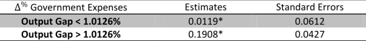
Government Expenses Estimates Standard Errors
Output Gap < 1.0126% 0.0119* 0.0612
Output Gap > 1.0126% 0.1908* 0.0427
11
Constant Term Estimate Standard Error
Output Gap < 1.0126% 0.0011* 0.0008
Table 15 - Regime Specific Constant Term Before 2009
Those last years changed a lot the behavior of the economy as this results show
exactly the opposite tendency regarding government expenses before the crisis.
Nonetheless, we must understand that only in 18 observations do we see
contractionary measures (understanding contractionary measures as reductions of
government expenses), which makes us look almost exclusively to how GDP reacted to
expansionary measures during the so-called Great Moderation, this creates sort of a
puzzle because it is not easy to understand why economies tended to deviate from
equilibrium in a positive way.
However, this can be interpreted as one of the reasons why the crisis was so
hard to overtake. Constantly overheated economies for a long time generate bubble
effects way more easily and it is undeniable that during the period that we are
considering, we had several markets, especially the real estate market, living in an
economic bubble (Lewis, 2010).
6.4. Just Crisis
If it is interesting to look at what happened before the crisis, it is also
interesting to look at what happened afterwards.
In this period, GDP decreased in several countries in several moments and
economies were constantly facing negative output gaps. It is a period where
economists were using trial and error in an attempt to surpass the problem because
this was an all-new phenomenon.
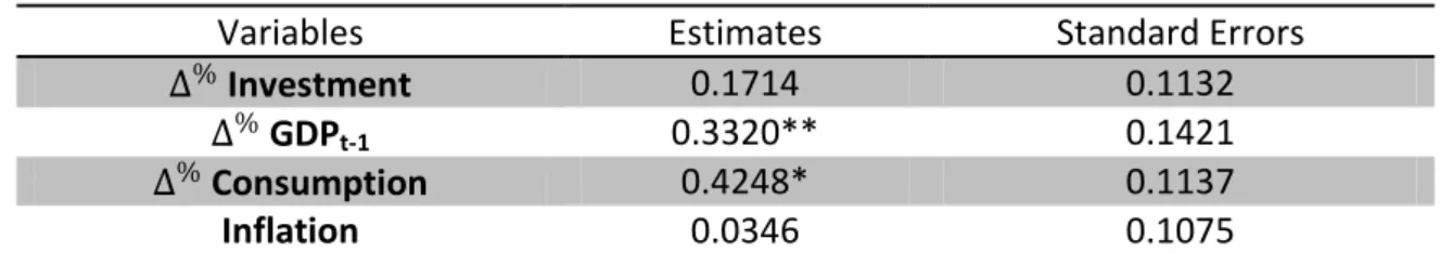
In this period we can see increases and decreases of all variables that we use in
our model and it has a great weight on the way that our main results are presented
because these periods correspond to almost half of the whole sample.
Threshold Value 95% Confidence Interval -0.9041% -6.6190% – -0.3946%
Table 16 - Threshold Value After 2009
Variables Estimates Standard Errors
Investment 0.1714 0.1132
GDPt-1 0.3320** 0.1421
Consumption 0.4248* 0.1137
12
Real Ex. Rate -0.0675 0.0472
Population -0.1645 0.1787
Table 17 - Regime Independent Variables After 2009
Government Expenses Estimates Standard Errors
Output Gap < -0.9041% 0.1314* 0.0446
Output Gap > -0.9041% -0.0035 0.0587
Table 18 - Regime Dependent Variable After 2009
Constant Term Estimate Standard Error
Output Gap < -0.9041% 0.0017*** 0.0008
Table 19 - Regime Specific Constant Term After 2009
In this period, we see that the economy is mainly driven by changes in private
consumption and that fiscal policy is just significant when the output gap is below the
threshold level, reinforcing the conclusions of the main model with the whole sample.
However, during this period, economies passed three quarters of the whole
time below the threshold value.
7.
Conclusion
This work project tried to understand whether fiscal policy has different effects
in moments of positive or negative output gap. To do so, we used a panel data
threshold model allowing for endogenous regressors proposed by Kramer et al. (2012).
The objective was to study if the fiscal multiplier varies in a non-linear way.
That non-linearity was provided by the state of the economy, depending on whether
we were facing a positive or a negative output gap. Our purpose was to understand
what governments can do when facing a recession period.
Considering the whole sample, we found what other studies often unveil:
namely that fiscal policy is stronger when potential GDP is higher than actual GDP and,
in our case, only in this scenario is fiscal policy significant to variations in GDP.
Our results suggest a threshold value of -0.7307% for the output gap, when the
economy shifted from one regime to another, dividing the sample into two regimes. In
the negative regime (calling negative regime the one where the output gap was below
the threshold value), the fiscal multiplier was 0.102, which means that whenever
governments raise their expenses in 1 p.p., ceteris paribus, GDP grwoth increased by
0.102 p.p., whereas, in the positive regime, the fiscal multiplier found was 0.036,
13
Nevertheless, since we studied 15 EU countries in the period between 2000 and
2016, one could easily imagine that this sample is quite troubled because of the crisis.
So we performed two kinds of robustness checks: one with and another without the
“PIGS” countries and one with the years after and another with the years before 2009.
In the first case, we found that without the “PIGS”, our model still behaves in
the same way, the threshold value remains the same and the fiscal multiplier even gets
larger in the negative regime. However, when studying just the PIGS, we get a smaller
threshold value (-3.07%) and find that when the output gap is below the threshold, the
fiscal multiplier is not significant. One possible explanation for this is that these
countries faced periods of austerity while their GDP was already significantly below its
potential.
In the second case, removing the years after 2009, the threshold value
becomes 1.01% and government expenses are significant and positive when the
output gap is larger than that value, which is contrary to the previous findings. An
explanation for this is that this period was marked by overheated economies and
expansionary measures, which created a bubble effect that distorted the results. When
looking at the sample from 2009 onwards, we find that our conclusions hold. In this
case, the threshold value is -0.90% and fiscal policy is only significant when the output
gap is below that value.
Our analysis would benefit from a larger sample. Unfortunately, many countries
did not collect quarterly data before 2000. One interesting development for future
work is the estimation of a panel data threshold Vector Autoregressive Model
combining all the literature that is being developed in the Threshold Vector
Autoregressive Models with the work of Hansen (1999, 2000) in the context of panel
data threshold models.
8.
References
Afonso A, Baxa J, Slavik M. 2011. Fiscal developments and financial stress: a threshold
VAR analysis. ECB working paper series 1319, European Central Bank.
Almunia M, Bénétrix A, Eichengreen B, O’Rourke KH, Rua G. 2010. From Great
Depression to Great Credit Crisis: similarities, differences and lessons. Economic Policy
25: 219–265.
Arellano M, Bover O. 1995. Another look at the instrumental variables estimation of
14
Bachmann R, Sims ER. 2012. Confidence and the transmission of government spending
shocks. Journal of Monetary Economics 59: 235–249.
Baum A, Checherita-Westphal C, Rother P. 2012a. Debt and growth: new evidence for
the euro area. ECB working paper series 1450, European Central Bank.
Baum A, Poplawski-Ribeiro M, Weber A. 2012b. Fiscal multipliers and the state of the
economy. Working paper 12/286, IMF.
Blanchard O, Perotti R. 2002. An empirical characterization of the dynamic effects of
changes in government spending and taxes on output. Quarterly Journal of Economics
117: 1329–1368.
Candelon B, Lieb L. 2013. Fiscal policy in good and bad times. Journal of Economic
Dynamics and Control 37: 2679–2694.
Caner M, Hansen B. 2004. Instrumental Variable Estimation of a Threshold Model.
Journal of Economic Theory 20: 813-843.
Caselli F, Esquivel G, Lefort F. 1996. Reopening the convergence debate: a new look at
cross-country growth empirics. Journal of Economic Growth 1(3): 363-389.
Chang C, Khamkaew T, McAleer M. 2009. A Panel Threshold Model of Tourism
Specialization and Economic Development.
http://www.cirje.e.u-tokyo.ac.jp/research/dp/2009/2009cf685.pdf (visited on 30th November 2016)
Corsetti G, Meier A, Müller G. 2012. What determines government spending
multipliers? Economic Policy 27: 521–565.
DeLong JB, Summers LH. 2012. Fiscal policy in a depressed economy. Working paper,
Brookings Institution.
Ferraresi T, Roventini, A, Fagiolo G. 2014. Fiscal Policies and Credit Regimes: A TVAR
Approach. Journal of Applied Econometrics 30: 1047-1072
Galí J, López-Salido JD, Vallés J. 2007. Understanding the effects of government
spending on consumption. Journal of the European Economic Association 5: 227–270.
Hansen B. 1999. Threshold effects in non-dynamic panels: estimation, testing, and
15
Hansen B. 2000. Sample splitting and threshold estimation. Econometrica 68(3):
575-603.
Jorgenson D. 1963. Capital Theory and Investment Behavior.
https://assets.aeaweb.org/assets/production/journals/aer/top20/53.2.247-259.pdf
(visited on 30th November 2016)
Lewis, M. 2010. The Big Short: Inside The Doomsday Machine. W. W. Norton &
Company.
Nunes L, Poirier R. 2014. Fiscal Multipliers in Portugal Using a Threshold Approach.
https://run.unl.pt/bitstream/10362/11536/1/Poirier_2014.pdf (visited on 30th
November 2016).
Ramey V. 2011b. Identifying government spending shocks: it’s all in the timing.
Quarterly Journal of Economics 126: 1–50.
Romer C, Romer D. 2010. The macroeconomic effects of tax changes: estimates based
16
9.
Appendix
9.1. Descriptive Statistics
All statistics are based in quarterly changes.
Output Gap MEAN MAX MIN MEDIAN STD. DEV.
Austria -0.12% 3.75% -3.67% -0.36% 2.00%
Belgium -0.02% 2.94% -2.15% -0.14% 1.30%
Denmark -0.04% 4.52% -3.61% -0.75% 2.38%
Finland -0.42% 6.02% -4.88% -0.45% 2.83%
France -0.05% 2.89% -3.00% -0.03% 1.63%
Germany -0.34% 3.01% -4.79% -0.09% 1.68%
Greece -1.54% 9.77% -14.48% 0.17% 7.89%
Ireland 1.56% 10.37% -8.62% 4.27% 6.94%
Italy -0.94% 2.89% -4.98% 0.13% 2.71%
Luxembourg -0.13% 6.01% -4.12% -0.23% 2.09%
Netherlands -0.40% 3.99% -3.53% -0.92% 2.24%
Portugal -1.62% 4.45% -8.07% -0.43% 3.63%
Spain -0.52% 5.58% -7.99% 1.93% 4.28%
Sweden -0.30% 4.78% -6.24% -0.68% 2.51%
United Kingdom -0.27% 4.21% -4.56% 0.14% 2.32%
Table 20 - Output Gap Descriptive Statistics
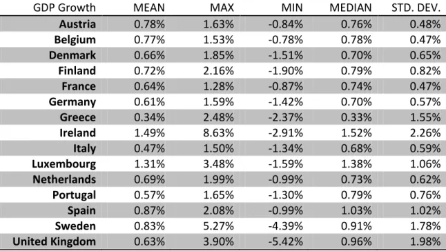
GDP Growth MEAN MAX MIN MEDIAN STD. DEV.
Austria 0.78% 1.63% -0.84% 0.76% 0.48%
Belgium 0.77% 1.53% -0.78% 0.78% 0.47%
Denmark 0.66% 1.85% -1.51% 0.70% 0.65%
Finland 0.72% 2.16% -1.90% 0.79% 0.82%
France 0.64% 1.28% -0.87% 0.74% 0.47%
Germany 0.61% 1.59% -1.42% 0.70% 0.57%
Greece 0.34% 2.48% -2.37% 0.33% 1.55%
Ireland 1.49% 8.63% -2.91% 1.52% 2.26%
Italy 0.47% 1.50% -1.34% 0.68% 0.59%
Luxembourg 1.31% 3.48% -1.59% 1.38% 1.06%
Netherlands 0.69% 1.99% -0.99% 0.73% 0.62%
Portugal 0.57% 1.65% -1.30% 0.79% 0.76%
Spain 0.87% 2.08% -0.99% 1.03% 1.02%
Sweden 0.83% 5.27% -4.39% 0.91% 1.78%
United Kingdom 0.63% 3.90% -5.42% 0.96% 1.98%
17
Government Expenses Growth MEAN MAX MIN MEDIAN STD. DEV.
Austria 0.87% 2.09% -0.54% 0.82% 0.52%
Belgium 1.01% 2.19% 0.27% 0.94% 0.45%
Denmark 0.82% 1.98% -0.41% 0.89% 0.56%
Finland 1.05% 2.14% -0.09% 1.11% 0.53%
France 0.76% 1.57% 0.26% 0.77% 0.31%
Germany 0.68% 1.57% -0.34% 0.69% 0.40%
Greece 0.51% 3.30% -4.25% 1.52% 2.10%
Ireland 1.22% 4.40% -2.82% 1.18% 1.72%
Italy 0.58% 2.22% -0.78% 0.30% 0.89%
Luxembourg 1.60% 3.00% -0.20% 1.69% 0.71%
Netherlands 1.04% 2.78% -0.39% 0.83% 0.89%
Portugal 0.51% 2.32% -3.54% 0.71% 1.29%
Spain 1.10% 2.53% -3.26% 1.61% 1.24%
Sweden 0.92% 4.18% -2.74% 1.00% 1.43%
United Kingdom 0.87% 3.69% -3.19% 1.37% 1.64%
Table 22 – Government Expenses Growth Descriptive Statistics
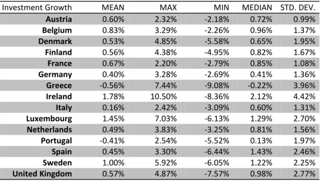
Investment Growth MEAN MAX MIN MEDIAN STD. DEV.
Austria 0.60% 2.32% -2.18% 0.72% 0.99%
Belgium 0.83% 3.29% -2.26% 0.96% 1.37%
Denmark 0.53% 4.85% -5.58% 0.65% 1.95%
Finland 0.56% 4.38% -4.95% 0.82% 1.67%
France 0.67% 2.20% -2.79% 0.85% 1.08%
Germany 0.40% 3.28% -2.69% 0.41% 1.36%
Greece -0.56% 7.44% -9.08% -0.22% 3.96%
Ireland 1.78% 10.50% -8.36% 2.12% 4.42%
Italy 0.16% 2.42% -3.09% 0.60% 1.31%
Luxembourg 1.45% 7.03% -6.13% 1.29% 2.70%
Netherlands 0.49% 3.83% -3.25% 0.81% 1.56%
Portugal -0.41% 2.54% -5.52% 0.13% 1.97%
Spain 0.45% 3.30% -6.44% 1.43% 2.46%
Sweden 1.00% 5.92% -6.05% 1.22% 2.25%
United Kingdom 0.57% 4.87% -7.57% 0.98% 2.77%
18
Consumption Growth MEAN MAX MIN MEDIAN STD. DEV.
Austria 0.73% 1.53% 0.05% 0.68% 0.36%
Belgium 0.71% 1.48% -0.45% 0.63% 0.42%
Denmark 0.72% 2.00% -1.09% 0.72% 0.57%
Finland 0.95% 1.90% -0.57% 1.03% 0.53%
France 0.65% 1.40% -0.54% 0.73% 0.44%
Germany 0.50% 1.06% -0.37% 0.52% 0.27%
Greece 0.41% 2.58% -2.65% 0.83% 1.53%
Ireland 0.92% 2.92% -3.38% 1.29% 1.43%
Italy 0.48% 1.32% -0.67% 0.63% 0.50%
Luxembourg 0.92% 2.53% -0.14% 0.96% 0.53%
Netherlands 0.50% 1.48% -1.14% 0.49% 0.52%
Portugal 0.62% 1.75% -1.44% 0.93% 0.86%
Spain 0.81% 2.04% -1.63% 0.81% 0.96%
Sweden 0.75% 4.40% -3.36% 0.83% 1.56%
United Kingdom 0.57% 3.90% -5.05% 0.82% 1.93%
Table 24 – Private Consumption Growth Descriptive Statistics
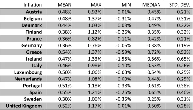
Inflation MEAN MAX MIN MEDIAN STD. DEV.
Austria 0.48% 0.92% 0.01% 0.45% 0.21%
Belgium 0.48% 1.37% -0.31% 0.47% 0.31%
Denmark 0.44% 1.03% 0.03% 0.49% 0.22%
Finland 0.38% 1.12% -0.26% 0.35% 0.32%
France 0.36% 0.82% -0.11% 0.42% 0.21%
Germany 0.36% 0.76% -0.06% 0.38% 0.19%
Greece 0.54% 1.37% -0.59% 0.72% 0.52%
Ireland 0.47% 1.33% -1.55% 0.56% 0.65%
Italy 0.46% 0.98% -0.10% 0.53% 0.26%
Luxembourg 0.50% 1.06% -0.03% 0.54% 0.25%
Netherlands 0.47% 1.08% 0.00% 0.44% 0.25%
Portugal 0.51% 1.18% -0.38% 0.61% 0.38%
Spain 0.55% 1.21% -0.26% 0.65% 0.40%
Sweden 0.30% 1.06% -0.35% 0.25% 0.31%
United Kingdom 0.52% 1.17% -0.01% 0.50% 0.28%
19
Real Ex. Rate Perc. Change MEAN MAX MIN MEDIAN STD. DEV.
Austria 0.05% 1.13% -1.14% 0.10% 0.52%
Belgium 0.11% 1.26% -1.49% 0.12% 0.58%
Denmark 0.07% 1.74% -1.73% 0.08% 0.72%
Finland 0.06% 1.87% -2.16% 0.11% 0.86%
France 0.02% 1.87% -1.87% 0.11% 0.76%
Germany -0.02% 1.64% -1.92% 0.05% 0.77%
Greece 0.10% 2.06% -2.15% 0.18% 0.76%
Ireland 0.12% 2.89% -2.62% 0.40% 1.18%
Italy 0.11% 2.06% -1.79% 0.18% 0.79%
Luxembourg 0.17% 1.37% -1.03% 0.23% 0.45%
Netherlands 0.10% 1.44% -1.48% 0.06% 0.66%
Portugal 0.11% 1.53% -1.18% 0.13% 0.58%
Spain 0.17% 1.89% -1.72% 0.28% 0.67%
Sweden -0.08% 2.88% -3.85% 0.08% 1.48%
United Kingdom -0.16% 2.12% -5.36% -0.04% 1.47%
Table 26 – Real Exchange Rate Percentage Change Descriptive Statistics
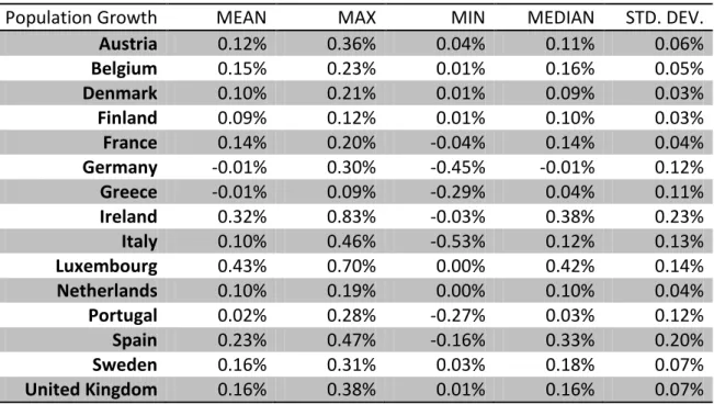
Population Growth MEAN MAX MIN MEDIAN STD. DEV.
Austria 0.12% 0.36% 0.04% 0.11% 0.06%
Belgium 0.15% 0.23% 0.01% 0.16% 0.05%
Denmark 0.10% 0.21% 0.01% 0.09% 0.03%
Finland 0.09% 0.12% 0.01% 0.10% 0.03%
France 0.14% 0.20% -0.04% 0.14% 0.04%
Germany -0.01% 0.30% -0.45% -0.01% 0.12%
Greece -0.01% 0.09% -0.29% 0.04% 0.11%
Ireland 0.32% 0.83% -0.03% 0.38% 0.23%
Italy 0.10% 0.46% -0.53% 0.12% 0.13%
Luxembourg 0.43% 0.70% 0.00% 0.42% 0.14%
Netherlands 0.10% 0.19% 0.00% 0.10% 0.04%
Portugal 0.02% 0.28% -0.27% 0.03% 0.12%
Spain 0.23% 0.47% -0.16% 0.33% 0.20%
Sweden 0.16% 0.31% 0.03% 0.18% 0.07%
United Kingdom 0.16% 0.38% 0.01% 0.16% 0.07%