4
Novembro de 2013
TEXTO DE DISCUSSÃO Nº37
ESTIMATING THE OUTPUT GAP:
A SVAR Approach
Vinícius de Oliveira Botelho
Samuel de Abreu Pessoa
Estimating the Output Gap: a SVAR Approach
∗
Vin´ıcius de Oliveira Botelho (IBRE FGV)
Samuel de Abreu Pessoa (IBRE FGV)
Silvia Maria Matos (IBRE FGV)
November 8, 2013
1
Introduction
The output gap measurement is one of the most difficult and important subjects in applied macroeconomics. It not only allows us to estimate the relationship between inflation and economic activity but also to evaluate the impact of inter-est rates movements and fiscal expansions on prices. There are three common strategies for estimating it: statistical filtering (e.g., the HP filter), production function approach, and demand shocks identification (such as Blanchard and Quah, in [4]). We use a combination of the second and third ones, applying the methology developed by [2] to identify demand shocks using the set of variables implied by the production function approach (and an external component).
2
Methodology
The variables were chosen to approximate a Cobb-Douglas production function (equation 1). Taking logs and derivatives of equation 1 and approximating the capital stock growth by the GDP’s gross investment, we have a relationship be-tween (HW) hours worked (IBRE), (CU) capacity utilization (IBRE), (GFCF) gross fixed capital formation (IBGE), (BGDP) Brazilian GDP (IBGE), and (UGDP) US GDP (BEA). Hence, these are the chosen variables for our SVAR. All data are quarterly (2004Q1 to 2013Q2) and seasonally adjusted.
GDPt=P rodt(Kt(1−N U CIt)) α
(Hourst))
1−α
(1)
The VAR, introduced by [5], has the form of equation 2: a set of simulta-neous equations explaining each of the variables from the vectorYt as a linear
combination of all variables fromYt−1up toYt−k and a constant1.
∗The views expressed here are from its author and do not represent the official opinions of
FGV or IBRE
1Note that the lagged terms ofYt are exogenous toYt (Ytcannot have causal impact on
Yt=β0+
k
X
j=1
Yt−jβj+Aut (2)
In equation 2, ut is a 5x1 vector of shocks and A is a 5x5 matrix that
contemporaneously transmits the shocks in each of these 5 variables to all of them. However, the VAR estimation provides only residuals (its coefficients,βj,
are estimated under OLS and the residualsutare the difference between actual
Yt and predicted values forYt), not the structural shocks series. In order to
identify them, assumptions on matrixAare needed.
A will be estimated by covariance-matching. The residual covariance of equation 2 is given byE[Autu′tA′], and we know that, beingCov the estimated
variance-covariance matrix, Cov = E[Autu′tA′] (supposing A is deterministic
and E[utu′t] = I, Cov = AA′). Cov has 25 values and A has 25 variables;
however, Cov and AA′ are symmetric. Therefore, while Cov = AA′ has 25 equations, only 15 of them are linearly independent (the 10 on the superior triangle are identical to the 10 on the inferior one). As a consequence, we need to impose 10 identification restrictions in order to have 25 equations for 25 variables (15 come from Cov = AA′ and 10 come from the identification restrictions).
These restrictions are on the short run and long run properties of our shocks (following [2]). They are:
• 1) Brazil is a small open economy
• 2) An increase in GDP may be caused by an increase in the hours worked, but not the opposite
• 3) An increase in GDP may be caused by an increase in the NUCI, but not the opposite
All restrictions are imposed to A: short run restrictions have the form of equation 3 (ai,jis the element ofAon thei-th row andj-th column), while long
run restrictions have the form of equation 4 (LRi,j is the element ofLRon the
i-th row andj-th column).
ai,j= 0 (3)
LR= (I−
Xk
j=1βj)−1AT
LRi,j = 0
(4)
comprises two more restrictions (GDP and investment do not affect neither the number of hours worked nor the NUCI). All identification conditions can be summarized in the system of equations 5.
aBGDP,HW = 0 (Condition2)
aBGDP,CU = 0 (Condition3)
aHW,U GDP = 0 (Condition1)
aCU,U GDP = 0 (Condition1)
aGF CF,U GDP = 0 (Condition1)
LRBGDP,HW = 0 (Condition2)
LRBGDP,CU = 0 (Condition3)
LRHW,U GDP = 0 (Condition1)
LRCU,U GDP = 0 (Condition1)
LRGF CF,U GDP = 0 (Condition1)
(5)
After the identification of the elements ofAwe can compute the shocks that hit the economy for each period in our sample. This can be easily done using equation 6 (etis the residual of the VAR described in equation 2).
ut=A−1et (6)
Therefore, we can calculate Brazilian GDP if only some of the five shocks occurred. Hence, using the decomposition method introduced by [1] we can calculate the contribution to economic growth for each of the 5 variables in our VAR. The first two variables (hours worked and NUCI) are interpreted as demand shocks, and so generate the output gap (the demand contribution to GDP growth is defined as the sum of the contributions of hours worked and NUCI). Similarly, the contribution of foreign shocks to the domestic growth are interpreted as the external gap. It is a natural consequence of this approach that the potential output be defined as the predicted value for GDP summed by the productivity and investment shocks.
3
The Output Gap
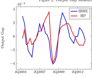
In figure 1 we show our estimates for the output gap. Since it captures demand shocks, it is indeed a very volatile series. In order to analyze our estimates, in figure 2 we show our four-quarter accumulated output gap and compare it with that obtained from the HP Filter. Both reflect percent deviations from the potential output. Interestingly, even our accumulated output gap is more volatile than the output gap derived from the HP Filter.
Figure 1: Output Gap Measures
1Q2004 3Q2006 1Q2009 3Q2011 2Q2013
−2 −1 0 1 2 ·10
−2
O
u
tp
u
t
G
ap
while ours immediately shows a rapid decline (there are negative demand shocks on 1Q2008, 3Q2008, and a strong negative shock in 4Q2008 and 1Q2009). Only in 4Q2008 the output gap derived from the HP is capable of indicating a deteri-oration in the aggregate demand. More importantly, after 2Q2012 the HP filter indicates a deflationary output gap, while our model shows there is inflationary pressure from aggregate demand. This is compatible with the rise in interest rates initiated in 2Q2013.
Figure 2: Output Gap Measures
4Q2004 2Q2007 4Q2009 2Q2012
−4 −2 0 2 4
·10−2
O
u
tp
u
t
G
ap
4
Small Economy Model (SEM)
Our SEM has 4 equations: the IS curve, the Phillips curve, the Taylor Rule, and the Expectations Rule. The Expectations Rule ensures that, in the long run, expected inflation equals actual inflation. The IS curve establishes a link between the neutral real interest rateex-ante and the long run nominal public deficit. It also determines the impact of the real interest rate and external output gap on the domestic one. The equations were estimated using GMM with lagged variables as regressors.
4.1
Phillips Curve
The Phillips Curve is vertical in the long run and depends on expectations, output gap, and the ERPT (exchange rate pass-through). Its reduced-form is expressed in equation 7, whereqtis the real exchange rate int,Htis the output
gap int,H∗
t is the foreign output gap int, Π t+3
t is inflation accumulated from
t to t+ 3, Et(xt+1) is the expectation operator for the random variable xt+1
based on an information set that comprises data only up to datet.
Πt=α0Πt−1+α1Πt−2+ (1−α0−α1)Et(Πtt+4+1)+
k1
X
j1=0
βj1Ht−j1+
k2
X
j2=0
γj2∆qt−j2+u
P t
(7)
Note that, in the long run, Ht, H∗t, and ∆qt are zero. It was estiamted
using GMM, with lagged variables as instruments. Πt is a core CPI measure.
Monitored and food prices are exogenous.
Table 1: Phillips Curve estimates
Variable Value
α0 1.070
(0.141)
α1 -0.266
(0.132)
β3 0.295
(0.102)
γ4 0.026
(0.009)
As table 1 suggests2, these estimates indicate a short run exchange-rate
pass-through (ERPT) of about 2.6% and very strong inertial effects. This is in
2Standard erros in parentheses. All ommitted parameters were statistically insignificant
part due to the fact that inflation was measured as four-quarter accumulated inflation.
4.2
IS
The IS equation follows the process described in 8.
Ht=c+αRrt+ f1
X
w1=1
ξw1Ht−w1+
f2
X
w2=0
ζw2H ∗
t−w2+
f3
X
w3=0
ηw3gt−w3+u
H t (8)
AlthoughHtandH∗t are zero in the long run,gtis not. Therefore, there is
a long run relationship between the real interest rate and the nominal deficit, as proportion of GDP.
Table 2: IS estimates
Variable Value
αR -0.110
(0.033)
ξ2 0.360
(0.057)
ζ0 0.502
(0.079)
η0 0.135
(0.060)
η2 0.113
(0.054)
As noted previously, for each level of permanent nominal deficit there is a real interest rate of equilibrium. For instance, for a nominal deficit of 2.8% of GDP, the real equilibrium interest rate is 6.3%; for a nominal deficit of 1.8% of GDP the real interest rate goes down to 4.1%.
The most recent data indicates a nominal deficit around 2.8% of GDP, which indicates a real interest rate of equilibrium lying around 6.3%. Therefore, the output gap calculated by this methodology seems to respond well to movements in interest rates and nominal government deficits, as expected.
Figure 3: Interest Rates and Nominal Deficits
1 2 3 4
2 4 6 8
Nominal Deficit (% of GDP)
R
eal
In
te
re
st
R
at
e
Also, the IRF (impulse response function) of four-quarter accumulated infla-tion after a shock of one standard deviainfla-tion (0.8%) on the output gap is shown in figure 4.
Figure 4: 4Q accumulated inflation after a 1 standard deviation shock on the output gap
0 10 20 30 40
0 0.1 0.2 0.3 0.4
t
In
fl
at
4.3
Taylor Rule
The monetary authority follows an inflation-targeting regime, defining the nom-inal interest rate. Therefore, as usual, it defines the level of inflation that will prevail in the long run (the inflation target). It assumes the relationship ex-pressed in 9, where ¯Π is the inflation target andui
tis a monetary policy shock.
it=γRit−1+ (1−γR)(i∗+λΠ(Πt−Π) +¯ λYHt) +uit (9)
Note that i∗ is the nominal interest rate of equilibrium (derived from the inflation target and the real interest rate of equilibrium), a clearly identified parameter in our model.
In the simulations, the real interest rate is computed using equation 10.
rt=
1 +it
1 +Et(Πt
+4
t+1)
−1 (10)
Table 3: Taylor Rule estimates
Variable Value constant -1.800 (0.527)
γR 0.951
(0.030)
λΠ 0.416
(0.076)
λY 0.533
(0.137)
The Taylor Rule estimates an inflation target of 5.49% and greater sensitiv-ity of the interest rate to output gap movements. This kind of sensitivsensitiv-ity is not usually found in the literature, but it may be the result of a more accurate mea-surement of the output gap, since it is widely known that erratic meamea-surement errors tend to underestimate their parameters.
4.4
Expectations
Expectations are assumed to be adaptative, as expressed in 11. This reduced form ensures that, in the long run,Et(Πtt+4+1) = Π
t+4
t+1.
Et(Πtt+4+1)−Et−4(Πtt−3) =λ(Π
t
t−3−Et−4(Πtt−3)) +u
E
Table 4: Expectation Rule estimates
Variable Value
λ 0.450
(0.077)
5
Results
5.1
Growth Decomposition
The model allows us to decompose the steady-state deviations in four com-ponents: external, productivity, demand, and investment. The results for the period 2007Q1 up to 2013Q2 are in figure 5.
Figure 5: Decomposition of the steady-state deviation of GDP growth
Note that, as expected, in the global economic crisis of 2008, global growth is the main cause of the plunge in Brazilian GDP. Also, in 2012 the external component seems to be an important driver of our low growth (in contrast with 2011, when it seems to be caused by negative productivity shocks).
5.2
Impulse Response Functions (IRFs)
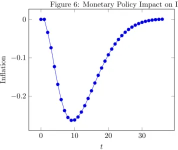
the nominal deficit is increased by 100 basis points for 4 quarters, going back to its original values after that, inflation will respond as in figure 7. The impacts estimated by this model are much greater than the ones showed in the Brazilian March Inflation Report ([3]).
Figure 6: Monetary Policy Impact on Inflation
0 10 20 30
−0.2 −0.1 0
t
In
fl
at
ion
This is a very striking result, since the nominal deficit has the operational (which impacts GDP and inflation) and the non-operational (which does not impact GDP and inflation) components: inasmuch as it suffers from this mea-surement error, its impacts tend to beunderestimated(bias toward zero). Other important observation is that a 100 basis points rise in the nominal deficit is much more unlikely than a 100 bps hike in the Selic. In fact, in our samples, a shock of one standard deviation in each of these variables would be a 350 bps hike in the Selic rate and a 140 bps hike in the nominal deficit. Therefore, although the Selic IRF shows an impact of approximately 0.25 bps after 9 quar-ters while the nominal deficit goes up to 0.40 bps, interest-rate movements are responsible for much more inflation fluctuation than the fiscal deficit (since it is 2.5 times more volatile).
Figure 7: Fiscal Policy Impact on Inflation
0 10 20 30
−0.4 −0.3 −0.2 −0.1 0
t
In
fl
at
ion
References
[1] Altissimo F. et al.Dealing with forward-looking expectations and policy rules in quantifying the channels of transmission of monetary policy. Economic Working Papers, 2002, Bank of Italy.
[2] Bjornland, Hilde C.; Leitemo, KaiIdentifying the interdependence between US monetary policy and the stock market. Journal of Monetary Economics, n.56 (2009), issue 2 (March), pages 275-282.
[3] Brazilian Central BankMarch Inflation Report. n.15 (2013), issue 1 (March).
[4] Blanchard, Olivier Jean; Quah, Danny The Dynamic Effects of Aggregate Supply and Demand Disturbances The American Economic Review, v.79, n.4 (Sep.1989), pp.655-673.
6
Rio de Janeiro
Rua Barão de Itambi, 60 22231-000 - Rio de Janeiro – RJ
São Paulo
Av. Paulista, 548 - 6º andar 01310-000 - São Paulo – SP