A new approach to constrained total least squares image restoration

(1)

Linear Algebra and its Applications 316 (2000) 237–258

www.elsevier.com/locate/laa

A new approach to constrained total least squares

image restoration

ø

Michael K. Ng

a,∗,1

_{, Robert J. Plemmons}

b,2

_{, Felipe Pimentel}

c,3

a_{Department of Mathematics, The University of Hong Kong, Pokfulam Road, Hong Kong} b_{Department of Mathematics and Computer Science, Wake Forest University, Winston-Salem,}

NC 27109, USA

c_{Departamento de Matemática, Universidade Federal de Ouro Preto, Ouro Preto, Brazil}

Received 30 March 1999; accepted 17 March 2000 Submitted by X. Sun

Abstract

Recently there has been a growing interest and progress in using total least squares (TLS) methods for solving blind deconvolution problems arising in image restoration. Here, the true image is to be estimated using only partial information about the blurring operator, or point spread function (PSF), which is subject to error and noise. In this paper, we present a new iterative, regularized, and constrained TLS image restoration algorithm. Neumann boundary conditions are used to reduce the boundary artifacts that normally occur in restoration pro-cesses. Preliminary numerical tests are reported on some simulated optical imaging problems in order to illustrate the effectiveness of the approach, as well as the fast convergence of our iterative scheme. © 2000 Elsevier Science Inc. All rights reserved.

Keywords: Constrained total least squares; Toeplitz matrix; Neumann boundary condition; Deconvolu-tion; Regularization

ø _{The first and third authors would like to dedicate their work on this paper to Prof. Robert J.}

Plem-mons, in celebration of his 60th birthday.

∗ Corresponding author. Tel.: +852-28592252; fax: +852-25592225.

E-mail addresses:mng@maths.hku.hk (M.K. Ng), plemmons@mthcsc.wfu.edu (R.J. Plemmons).

1 _{Research supported in part by Research Grants Council grant no. HKU 7147/99P and HKU CRCG}

grant no. 10202720.

2 _{Research supported in part by the National Science Foundation under grant no. CCR-9732070.} 3 _{Research supported by Brazilian Government/CAPES in cooperation with Center for Research in}

Scientific Computation, North Carolina State University, Raleigh, NC, USA.

(2)

M.K. Ng et al. / Linear Algebra and its Applications 316 (2000) 237–258

1. Introduction

A fundamental issue in image enhancement or restoration is blur removal in the presence of observation noise. Recorded images almost always represent a degraded version of the original scene. A primary example is an image taken by an optical instrument recording light that has passed through a turbulent medium, such as the atmosphere. Here, changes in the refractive index at different positions in the atmosphere result in a non-planar wavefront [32]. In general, the degrada-tion by noise and blur is caused by fluctuadegrada-tions in both the imaging system and the environment.

In this important case, where the blurring operation is spatially invariant, the basic restoration computation involved is a deconvolution process that faces the usual difficulties associated with ill-conditioning in the presence of noise [4, Chapter 2]. The image observed from a shift invariant linear blurring process, such as an optical system, is described by how the system blurs a point source of light into a larger image. The image of a point source is called the point

spread function(PSF), which we denote byh. The observed image g is then the

result of convolving the PSF h with the “true” image f, and with noise present in g. The standard deconvolution problem is to recover the image f given the observed imageg and the PSF h, see the recent survey paper written by Banham and Katsaggelos [2].

In classical image restoration, the PSF is assumed to be known or adequately sampled [1]. However, in practice, one is often faced with imprecise knowledge of the PSF. For instance, in two-dimensional deconvolution problems arising in based atmospheric imaging, the problem consists of an image received by a ground-based imaging system, together with an image of a guide star PSF observed under the effects of atmospheric turbulence. Empirical estimates of the PSF can sometimes be obtained by imaging a relatively bright, isolated point source. The point source might be a natural guide star or a guide star artificially generated using range-gated laser backscatter, e.g., [3,14,25]. Notice here that the PSF as well as the image are degraded by blur and noise.

In the literature, blind deconvolutionmethods [7,17,20,30,35] have been devel-oped to estimate both the true imagefand the PSFhfrom the degraded imageg. In order to obtain a reasonable restored image, these methods require one to impose suitable constraints on the PSF and the image. In our image restoration applications, the PSF isnotknown exactly (e.g., it is corrupted by errors resulting from blur and/or noise). A review of optimization models for blind deconvolution can be found in a recent survey paper by Kundar and Hatzinakos [20].

(3)

astro-M.K. Ng et al. / Linear Algebra and its Applications 316 (2000) 237–258

imaging applications. In [18], Kamm and Nagy have proposed the use of the TLS method for solving Toeplitz systems arising from image restoration problems. They applied Newton and Rayleigh quotient iterations to solve the Toeplitz TLS prob-lems. A possible drawback of their approach is that the PSF in the TLS formulation is not constrained to be spatially invariant. Mesarovic et al. [26] have shown that_´ formulating the TLS problem for image restoration with the spatially invariant con-straint improves the restored image greatly, see the numerical results in [26], or in Section 5.

The determination of fgiven the recorded data gand knowledge of the PSF h

is an inverse problem [9]. Deconvolution algorithms can be extremely sensitive to noise. It is necessary to incorporate regularization into deconvolution to stabilize the computations. Regarding the regularization, Golub et al. [10] have shown how Tikhonov regularization methods, for regularized least squares computations, can be recast in a TLS framework, suited for problems in which both the coefficient matrix and the right-hand side are known only approximately. However, their results do not hold for the constrained TLS formulation [26]. Therefore, we cannot use the algorithm in [10].

In [26], the authors addressed the problem of restoring images from noisy mea-surements in both the PSF and the observed data as a regularized and constrained TLS problem. It was shown in [26] that the regularized minimization problem ob-tained is nonlinear and nonconvex. Thus fast algorithms for solving this nonlinear optimization problem are required. In [26], circulant, or periodic, approximations are used to replace the convolution matrices in subsequent computations. In the Fou-rier domain, the system of nonlinear equations is decoupled into a set of simplified equations and therefore the computational cost can be reduced significantly. How-ever, practical signals and images often do not satisfy these periodic assumptions and ringing effects will appear on the boundary [24].

In the image processing literature, various methods have been proposed to as-sign boundary values, see [21, p. 22] and the references therein. For instance, the boundary values may be fixed at a local image mean, or they can be obtained by a model-based extrapolation. In this paper, we consider the image formulation model for the regularized constrained TLS problem using theNeumann boundary condition

for the image, i.e., we assume that the scene immediately outside is a reflection of the original scene near the boundary. This Neumann boundary condition has been recently studied in image restoration [21,24,28] and in image compression [23,33]. Results in [28] show that the boundary artifacts resulting from the deconvolution computations are much less prominent than that under the assumption of zero [18] or periodic [26] boundary conditions.

(4)

transform. Our preliminary simulation results show that the regularized constrained TLS method with Neumann boundary condition is better than the regularized least squares method using the degraded PSF.

Our paper is outlined as follows. An algorithm for one-dimensional regularized, constrained TLS-based signal restoration with Neumann boundary conditions is de-veloped in Section 2. We devise a fixed-point iteration, which is an efficient method for restoring the original signal, in Section 3. The method is extended to two-dimen-sional imaging problems in Section 4. Numerical results are presented in Section 5. Our preliminary numerical results show that the restored image given by using the regularized, constrained TLS method with Neumann boundary conditions is often superior to that obtained by the least squares method. Our iterative scheme is also quite robust, and converges very fast.

2. One-dimensional deconvolution formulation

For simplicity, we begin with the one-dimensional deblurring problem. Consider the original signal

f₌(. . . , f₋n, f−n+1, . . . , f0, f1, . . . , fn, fn+1, . . . , f2n, f2n+1, . . .)t

and thediscrete PSFgiven by

h₌(. . . ,0,0, h₋n+1, . . . , h0, . . . , hn−1,0,0, . . .)t.

Here t denotes transposition. The blurred signal is the convolution ofhandf, i.e., theith entryg_¯i of the blurred signal is given by

¯ gi =

∞ X

j_=−∞

hi₋jfj. (1)

Therefore, the blurred signal vector is given by

¯

g_{= [ ¯}g1, . . . ,g¯n]t.

For a detailed discussion of digitizing images, see [4, Chapter 2]. From (1), we have



     

¯ g1

¯ g2

.. . ¯ gn−1

¯ gn



     

= 

     ¯

hn₋1 · · · h¯1 h¯0 · · · ¯h−n₊1 0

. .. .._. .._. _h_¯

−n₊1 ¯

hn−1 ... ... . ..

0 h¯n−1 · · · h¯0 h¯−1 · · · ¯h−n+1 

(5)

M.K. Ng et al. / Linear Algebra and its Applications 316 (2000) 237–258 ×                     

f₋n+2 .. . f0 − − − f1 .. . fn − − − fn₊1

.. . f2n−1

                    

= [ ¯Hl| ¯Hc| ¯Hr]

      fl −− fc −− fr      

= [ ¯Hl| ¯Hc| ¯Hr]f. (2)

Here _[A_|B_] denotes an m-by-(n1+n2)matrix, where A and B are m-by-n1 and

m-by-n2matrices, respectively.

For a givenn, the deconvolution problem is to recover the vector_[f1, . . . , fn]t

given the PSF h¯ and a blurred signalg_¯_{= [ ¯}g1, . . . ,g¯n]t of finite length n. Notice

that the blurred signalg_¯ is determined not only by fc= [f1, . . . , fn]t, but by f=

[flfcfr]t.

The linear system (2) is underdetermined. To recover the vectorfc, we assume the

data outsidefcare reflections of the data insidefc, i.e.,

  

 

f₀ ₌ f₁

..

. ... ... f₋n+2 = fn−1

and     

fn+1 = fn

..

. ... ... f2n−1 = f2

(3)

In [28], it has been shown that the use of this (Neumann) boundary condition can re-duce the boundary artifacts and that solving the resulting systems is much faster than using zero and periodic boundary conditions. The discussion of using the Neumann boundary condition can be found in [28].

In this paper, the PSF is not known exactly. Since the spatial invariance of h

translates into the spatial invariance of the noise in the blurring matrix. We assume that the “true” PSF can be represented by the following formula:

¯

h₌h₊δh, (4)

whereh_{= [}h₋n+1, . . . , hn−1]tis the estimated (or measured) PSF and

δh_{= [}δh₋n₊1, δh−n₊2, . . . , δh0, . . . , δhn₋2, δhn₋1]t

is the error component of the PSF. Eachδhi is modeled as independent

(6)

blurred signalg_¯ is also subject to errors. We assume that the observed signalg₌

[g1, . . . , gn]tcan be represented by

¯

g₌g₊δg, (5)

where

δg_{= [}δg1, δg2, . . . , δgn]t

andδgi is independent uniformly distributed noise with zero-mean and varianceσg2.

Here the noise in the PSF and in the observed signal are assumed to be uncorrelated. Thus, our image restoration problem is to recover the vectorf from the given inexact PSFhand a blurred and noisy signalg. In the next subsection, we develop our constrained TLS approach to solving the image restoration problem, using the one-dimensional case for simplicity of presentation.

2.1. Regularized and constrained TLS formulation

Using (4) and (5), the convolution equation (2) can be reformulated as follows:

Hf₋g₊δHf₋δg₌0, (6)

where

H ₌



    

hn−1 · · · h1 h0 · · · h−n+1 0

. .. .._. .._. _h

−n+1

hn−1 ... ... . ..

0 hn−1 · · · h0 h−1 · · · h−n+1 

    

= [Hl|Hc|Hr] (7)

and

δH ₌ 

    

δhn−1 · · · δh1 δh0 · · · δh−n+1 0

. .. .._. .._. _δh

−n+1

δhn−1 ... ... . ..

0 δhn−1 · · · δh0 δh−1 · · · δh−n+1 

    

= [δHl|δHc|δHr]. (8)

Correspondingly, we can define the Toeplitz matricesHl,HcandHr, andδHl,δHc

andδHr similar toH¯l,H¯candH¯r in (2), respectively. The constrained TLS

formu-lation amounts to determining the necessary “minimum” quantitiesδH andδgsuch that (6) is satisfied.

Mathematically, the constrained TLS formulation can be expressed as

min fc k[

(7)

subject to

Hf₋g₊δHf₋δg₌0,

wherefsatisfies (3).

Recall that image restoration problems are in general ill-conditioned inverse prob-lems and restoration algorithms can be extremely sensitive to noise [12, p. 282]. Regularization can be used to achieve stability. Using classical Tikhonov regular-ization [9, p. 117], stability is attained by introducing a regularregular-ization operatorD

and a regularization parameterµ to restrict the set of admissible solutions. More specifically, the regularized solutionfcis computed as the solution to

min fc {k[

δH_|δg_]k2_F₊µ_kDfck22} (9)

subject to

Hf₋g₊δHf₋δg₌0, (10)

andfsatisfies (3). The term_kDfck2₂is added in order to regularize the solution. The

regularization parameterµcontrols the degree of regularity (i.e., degree of bias) of the solution. In many applications [6,12,16],_kDfc_k2 is chosen to be theL2-norm kfc_k2or theH1-normkLfck2, whereLis a first-order difference operator matrix. In this paper, we only consider theL2andH1regularization functionals.

The theorem below characterizes our constrained, regularized TLS formulation of the one-dimensional deconvolution problem.

Theorem 1. Under the Neumann boundary condition (3), the regularized con-strained TLS solution can be obtained as thefcthat minimizes the functional

P (fc)=(Afc−g)tQ(fc)(Afc−g)+µftcDtDfc, (11) where A is an n-by-n Toeplitz-plus-Hankel matrix

A₌Hc+ [0|Hl]J+ [Hr|0]J, (12)

J is the n-by-n reversal matrix,

Q(fc)=([T (fc)|I][T (fc)|I]t)−1≡ [T (fc)T (fc)t+I]−1,

T (fc)is an n-by-(2n−1)Toeplitz matrix

T (fc)=

1 √_n



       

fn fn₋1 · · · f2 f1 f1 · · · fn₋2 fn₋1 fn fn . .. . .. f2 f1 . .. fn−3 fn−2

..

. . .. . .. . .. . .. . .. . .. . .. ...

f3 f4 . .. fn fn−1 . .. . .. f1 f1 f2 f3 · · · fn fn fn−1 · · · f2 f1



       

, (13)

(8)

Proof. From (10), we have

[T (fc)_|I_] √

nδh

−δg

=√nT (fc)δh₋δg₌δHf₋δg

=g₋Hf₌g₋Afc. (14)

We note that

k[δH_|δg_]k2_F₌n_kδh_k2₂_{+ k}δg_k2₂ ₌

√ nδh

−δg

2 2 .

Therefore, we obtain the minimum 2-norm solution of the underdetermined system in (14), see for instance [11]. Since the rank of the matrix_[T (fc)|I]isn, we have

√_nδ_h −δg

= [T (fc)|I]tQ(fc)(g−Afc)

or √ nδh

−δg

2 2

=(Afc−g)tQ(fc)(Afc−g). (15)

By inserting (15) into (9), we obtain (11).

2.2. Symmetric point spread functions

The estimates of the discrete blurring function may not be unique, in the absence of any additional constraints, mainly because blurs may have any kind of Fouri-er phase, see [21]. Nonuniqueness of the discrete blurring function can in genFouri-er- gener-al be avoided by enforcing a set of constraints. In many papers degener-aling with blur identification [7,13,22], the PSF is assumed to be symmetric, i.e.,

¯

hk= ¯h−k, k=1,2, . . . , n−1.

We remark that PSFs are often symmetric, see [16, p. 269], for instance, the Gaussian PSF arising in atmospheric turbulence induced blur is symmetric with respect to the origin. For guide star images [13], this is usually not the case. However, they often appear to be fairly symmetric, which can be observed by measuring their distance to a nearest symmetric PSF. In [13], Hanke and Nagy use the symmetric part of the measured PSF to restore atmospherically blurred images.

Similarly, we thus incorporate the following symmetry constraints into the TLS formulation of our problem:

¯

(9)

Then using Neumann boundary conditions (3), the convolution equation (6) becomes

Afc−g+δAfc−δg=0,

whereAis defined in (12) andδAis defined similarly. It was shown in [28] that these Toeplitz-plus-Hankel matricesAandδAcan be diagonalized by ann-by-ndiscrete cosine transform matrixCwith entries

Cij =

r 2₋δi1

n cos

_(i

−1)(2j₋1)π 2n

, 16i, j,6n,

whereδij is the Kronecker delta, see [16, p. 150]. We note thatCis orthogonal, i.e.,

CtC₌I. Also, for anyn-vectorv, the matrix–vector multiplicationsCv andCtv

can be computed in O(nlogn)real operations by fast cosine transforms (FCTs); see [31, pp. 59, 60].

In the following discussion, we write

A₌Ctdiag(w) C and δA₌Ctdiag(δw) C. (17)

Here for a general vectorv, diag(v) is a diagonal matrix with its diagonal entries given by

[diag(v)_]i,i=vi, i=1,2, . . . , n.

Using (17), we can give a new regularized constrained TLS formulation to this sym-metric case as follows.

Theorem 2. Under the Neumann boundary condition(3)and the symmetry con-straint(16),the regularized constrained TLS solution can be obtained as theˆfcthat minimizes the functional

P (ˆfc)=[diag(w)ˆfc− ˆg]t{[diag(ˆfc)|I][diag(ˆfc)|I]t}−1[diag(w)ˆfc− ˆg]

+µˆft_cKˆfc, (18)

where

ˆ

f₌Cf, g_ˆ₌Cg,

andKis an n-by-n diagonal matrix given by

K=CDtDCt,

and D is the regularization operator.

Proof. In this regularized TLS formulation, we minimize_k[δA_|δg_]k2_F₊µ_kDfck2₂

subject toAfc−g+δAfc−δg=0. SinceAandδAcan be diagonalized byC, the

constraint now becomes

diag(w)ˆfc− ˆg+diag(δw)ˆfc−δgˆ =0.

(10)

[diag(ˆfc)|I]

y

−δg_ˆ

=diag(ˆfc)y−δgˆ =diag(δw)ˆfc−δgˆ= ˆg−diag(w)ˆfc.

Hence, we have

y

−δg_ˆ

= [diag(ˆfc)|I]t{[diag(ˆfc)|I][diag(ˆfc)|I]t}−1(gˆ−diag(w)ˆfc). (19)

The diagonalization ofAbyCimplies that

k[δA_|δg_]k2_F_=kCtdiag(δw)C_k2_F_{+ k}Ctδg_ˆ_k2₂

=kdiag(δw)_k2_F_{+ k}δg_ˆ_k2₂ ₌

y

−δg_ˆ

2 2 .

Now, by using (19), it is easy to verify thatk[δA_|δg_]k2_F₊µ_kDfck2₂is equal to the

second member of (18).

We recall that when the L2 and H1 regularization functionals are used in the restoration process, the main diagonal entries ofKare just given by

Kii=1 and Kii=4 cos2

_(i −1)π

2n

, 16i6n,

respectively.

3. Numerical algorithms

In this section, we introduce an approach to minimizing (11). For simplicity, we let

oQ(fc)

ofi =



  

oQ11(fc) ofi · · ·

oQ1n(fc) ofi

..

. ...

oQn1(fc) ofi · · ·

oQnn(fc) ofi



   .

Hereo_Q_{j k}₍fc)/ofiis the derivative of the(j, k)th entry ofQ(fc)with respect tofi.

By applying the product rule to the matrix equality

Q(fc)[T (fc)T (fc)t+I] =I,

we obtain oQ(fc)

ofi = −

Q(fc)

o_{T (fc)T (fc)t+I}

ofi

Q(fc)

or equivalently

o_Q(_fc₎

o_f_i = −Q(fc)

_o_{T (}_fc₎

o_f_i T (fc) t₊_{T (}_f

c)

o_{T (}_fc₎t o_f_i

(11)

The gradientG(fc)(derivative with respect tofc) of the functional (11) is given by

G(fc)₌2AtQ(fc)(Afc₋g)₊2µDtDfc₊u(fc), where

u(fc)=



      

(Afc−g)toQ(_offc)

1 (Afc−g)

(Afc₋g)toQ(fc)

of2 (Afc−g)

.. . (Afc₋g)toQ(fc)

ofn (Afc−g)



       .

The gradient descent scheme yields

f(k_c +1)₌f(k)_c ₋τkG(f(k)c ), k=0,1, . . .

A line search can be added to select the step sizeτk in a manner which gives

suf-ficient decrease in the objective functional in (11) to guarantee convergence to a minimizer. This gives the method of steepest descent, see [8,19,27]. While numerical implementation is straightforward, steepest descent has rather undesirable asymptot-ic convergence properties whasymptot-ich can make it very ineffasymptot-icient. Obviously, one can apply other standard unconstrained optimization methods with better convergence properties, like the nonlinear conjugate gradient method or Newton’s method. These methods converge rapidly near a minimizer provided the objective functional de-pends smoothly onfc. Since the objective function in (11) is nonconvex, this results

in a loss of robustness and efficiency for higher order methods like Newton’s meth-od. Moreover, implementing Newton’s method requires the inversion of ann-by-n

unconstructed matrix, clearly an overwhelming task for any reasonable-sized image, for instance,n₌65,536 for a 256_×256 image. Thus, these approaches may all be unsuitable for our image restoration problem.

In this paper, we develop an alternative approach to minimizing (11). At a mini-mizer, we know thatG(fc)=0, or equivalently,

2AtQ(fc)(Afc−g)+2µDtDfc−u(fc)=0.

The iteration can be expressed as

h

AtQ(f(k)_c )A₊µDtD i

f(k_c+1)₌u(f (k) c )

2 +A

t_Q(_f(k)

c )g. (20)

Note that at each iteration, one must solve a linear system depending on the previous iteratef(k)c , to obtain the new iteratef(kc+1). We also find that

d(k)₌f(k_c+1)₋f(k)_c _{= −}1

2 h

AtQ(f(k)_c )A₊µDtDi−1G(f(k)_c ).

Hence the iteration is of quasi-Newton form, and existing convergence theory can be applied, see for instance [8,19]. Since the matrixQ(f(k)c )is symmetric positive

(12)

its eigenvalues bounded away from zero (because of the regularization), each step computes the descent directiond(k), and global convergence can be guaranteed by using the appropriate step size, i.e.,

f(k_c +1)₌f(k)_c ₋τk

2 h

AtQ(f(k)_c )A₊µDtDi−1G(f(k)_c ),

where

τk = argminτk_>₀P (f(k)_c +τkd(k)).

With our proposed iterative scheme, one must solve a symmetric positive definite linear system

h

AtQ(f(k)_c )A₊µDtDix₌b (21)

for some b at each iteration. Of course these systems are dense in general, but have structures that can be utilized. We apply a preconditioned conjugate gradient method to solving these linear systems. For each iteration, we need to compute a matrix–vector product(AtQ(f(k)c )A+µDtD)vfor some vectorv. Since the matrices AandAtare Toeplitz-plus-Hankel matrices, their matrix–vector multiplications can be done in O(nlogn)operations for anyn-vector, see for instance [5]. However, for the matrix–vector product

Q(f(k)_c )v_{≡ {[}T (f(k)_c )_|I_][T (f(k)_c )_|I_]t_}−1v, we need to solve another linear system

n

[T (f(k)_c )_|I_][T (f_c(k))_|I_]toz₌v. (22)

Notice that the matrix–vector multiplicationsT (f(k)c )yandT (f(k)c )tvcan also be

com-puted O(nlogn)operations for anyn-vectory. A preconditioned conjugate gradient method will also be used for solving this symmetric positive definite linear system.

3.1. Cosine transform based preconditioners

We remark that all matrices that can be diagonalized by the discrete cosine trans-form matrixCmust be symmetric [28], soCabove can only diagonalize matrices with symmetric PSFs for our problem. On the other hand, for nonsymmetric PSFs, we can construct cosine transform based preconditioners to speed up the convergence of the conjugate gradient method.

Given a matrixX, we define the optimal cosine transform preconditionerc(X)to be the minimizer of_kX₋Q_k2_F over allQthat can diagonalized byC, see [28]. In our case, the cosine transform preconditionerc(A)ofAin (12) is defined to be the matrixCtKCsuch thatKminimizes

kCtKC₋A_k2_F.

HereKis any nonsingular diagonal matrix. Clearly, the cost of computingc(A)−1y

(13)

for findingc(A). The cosine transform preconditionerc(A)is just the blurring matrix (cf. (12)) corresponding to the symmetric PSFsi ≡(hi +h₋i)/2 with the Neumann

boundary condition imposed. This approach allows us to precondition the symmetric positive definite linear system (21).

Next, we construct the cosine transform preconditioner for_{[T (f(k)c )|I][T (f(k)c )|I]t}

which exploits the Toeplitz structure of the matrix. We approximateT (fc)by

˜ T (fc)=

1 2n₋1



       

fn fn−1 · · · f2 f1 0 · · · 0

0 fn . .. ... f2 f1 . .. 0

..

. . .. . .. ... . .. . .. . .. ... ...

0 . .. fn fn₋1 . .. . .. f1 0

0 _{· · ·} _{· · ·} 0 fn fn₋1 · · · f2 f1 

        .

In [29], Ng and Plemmons have proved that if fc is a stationary stochastic

pro-cess, then the expected value ofT (fc)T (fc)t− ˜T (fc)T (˜ fc)t is close to zero. Since

˜

T (fc)T (˜ fc)t is a Toeplitz matrix,c(T (˜ fc)T (˜ fc)t)can be found in O(n)operations,

see [5]. However, the original matrix T (fc)T (fc)t is much more complicated and

thus the construction cost ofc(T (˜ fc)T (˜ fc)t)is cheaper than that ofc(T (fc)T (fc)t). It is clear that the cost of computingc(T (˜ fc))−1yfor anyn-vectoryis again O(nlogn) operations. It follows that the cost per each iteration in solving the linear systems (21) and (22) are O(nlogn)operations.

Finally, we remark that the objective function is simplified in the cosine transform domain when the symmetry constraints are incorporated into the TLS formulation. In accordance with Theorem 2, the minimization ofP (ˆfc)in (18) is equivalent to

min ˆ fi

"

(wiˆfi− ˆgi)2

ˆ

f2_i ₊1 +µKiiˆf 2

i

#

, 16i6n.

We note that the objective function is decoupled intonequations, each to be mini-mized independently with respect to one DCT coefficient ofˆfc. It follows that each

minimizer can be determined by a one-dimensional search method, see [27].

4. Two-dimensional deconvolution problems

(14)

TLS method is appropriate. In addition, the estimated PSF is generally degraded in a manner similar to that of the observed image [32].

Letf (x, y)andg(x, y)_¯ be the functions of the original and the blurred images, respectively. The image restoration problem can be expressed as a linear integral equation

¯

g(x, y)₌ Z Z

¯

h(x₋y, u₋v)f (y, v)dydv. (23)

The convolution operation, as is often the case in optical imaging, acts uniformly (i.e., in a spatially invariant manner) onf. We consider numerical methods for ap-proximating the solution to the linear restoration problem in discretized (matrix) form obtained from (23). For notation purposes we assume that the image isn-by-n, and thus containsn2pixels. Typically,nis chosen to be a power of 2, such as 256 or larger. Then the number of unknowns grows to at least 65,536. The vectorsfand ¯

grepresent the “true” and observed image pixel values, respectively, unstacked by rows. After discretization of (23), the blurring matrixH¯ defined byh¯is given by

¯ H₌      

H(n−1) _{· · ·} H(1) H(0) _{· · ·} H(−n+1) 0 . .. .._. .._. _H(−n+1)

H(n−1) ... ... . ..

0 H(n−1) _{· · ·} H(0) H(−1) _{· · ·} H(−n+1)

      (24)

with each subblockH(j )being an n-by-(2n₋1)matrix of the form given by (7). The dimensions of the discrete PSFhare 2n₋1 and 2n₋1 in thex-direction and

y-direction, respectively.

Applying Neumann boundary conditions, the resulting matrixAis a block-Toep-litz-plus-Hankel matrix with Toepblock-Toep-litz-plus-Hankel blocks. More precisely,

A₌         

A(0) A(−1) _{· · ·} _{· · ·} A(−n+1) A(1) _A(0) . .. . .. .._.

..

. . .. . .. . .. ...

..

. . .. . .. A(0) A(−1) A(n−1) _{· · ·} _{· · ·} A(1) A(0)

         +       

A(1) A(2) _{· · ·} A(n−1) 0

A(2) q q A(−n+1)

..

. q q q ...

A(n−1) q q A(−2)

(15)

with each blockA(j )being ann-by-nmatrix of the form given in (12). We note that the A(j )in (25) and theH(j )in (24) are related by (12). A detailed discussion of using the Neumann boundary conditions for two-dimensional problems can be found in [28].

Using a similar argument, we can formulate the regularized constrained TLS problems under the Neumann boundary conditions.

Theorem 3. Under the Neumann boundary condition (3), the regularized con-strained TLS solution can be obtained as thefcthat minimizes the functional

P (fc)=(Afc−g)t([T|I][T|I]t)−1(Afc−g)+µftcDtDfc, where T is ann2-by-(2n₋1)2block-Toeplitz-Toeplitz-block matrix

T ₌1 n



       

Tn Tn−1 · · · T2 T1 T1 · · · Tn−2 Tn−1

Tn Tn . .. . .. T2 T1 . .. Tn₋3 Tn₋2 ..

. . .. . .. . .. . .. . .. . .. . .. ...

T3 T4 . .. Tn Tn−1 . .. . .. T1 T1 T₂ T₃ _{· · ·} Tn Tn Tn−1 · · · T2 T1



       

and each subblockTj is an n-by-(2n−1)matrix of the form given by(7).

For a symmetric PSF, we have the following theorem.

Theorem 4. Under the Neumann boundary condition(3)and the symmetry con-straint

hi,j =hi,₋j =h₋i,j =h₋i,₋j,

the regularized constrained TLS solution can be obtained as theˆfc that minimizes the functional

P (fc)=[diag(w)ˆfc− ˆg]t{[diag(ˆfc)|I][diag(ˆfc)|I]t}−1[diag(w)ˆfc− ˆg]

+µˆft_cKˆfc,

whereˆf₌Cf,gˆ₌Cg,andKis an n-by-n diagonal matrix given byK=CDtDCt

and D is the regularization operator.

5. Numerical examples

(16)

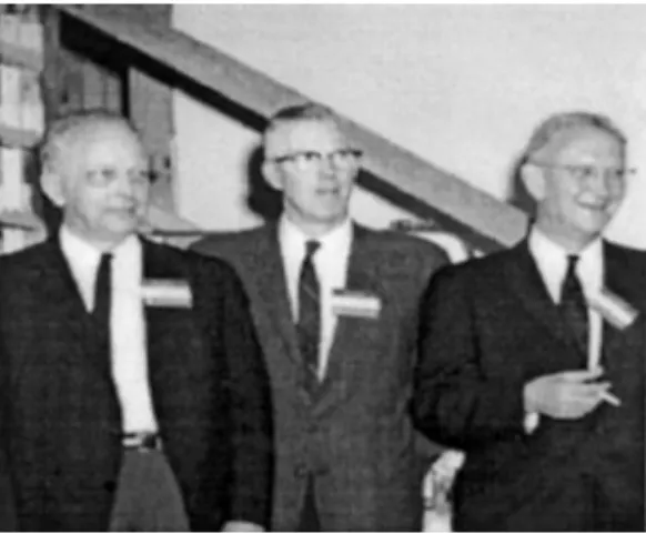
Fig. 1. “Gatlinburg Conference” test image.

right-hand side vectorg¯ correctly, we need the vectorsfl andfr, i.e., we need to

know the image outside the given domain. Thus we start with the 480-by-640 image of the photo and cut out a 256-by-256 portion from the image. Fig. 1(a) gives the 256-by-256 image of this picture.

We consider restoring the “Gatlinburg Conference” image blurred by a truncated (band limited) Gaussian PSF,

hi,j =

ce−0.1(i2+j2) _if_|_i₋_j_|₆₈_,

0 otherwise,

see [16, p. 269], wherehi,j is thejth entry of the first column ofA(i)in (25) andc

is the normalization constant such thatP

i,jhi,j =1. We remark that the Gaussian

PSF is symmetric, and is often used in the literature to simulate the blurring effects of imaging through the atmosphere [2,32]. Gaussian noise with signal-to-noise ratios of 40, 30 and 20 dB is then added to the blurred images and the PSFs to produce our test images. Noisy, blurred images are shown in Figs. 2(a) and 3(a). We note that after the blurring, the cigarette held by Prof. Householder (the rightmost person) is not clearly shown, cf. Fig. 1.

In Table 1, we present results for the regularized constrained TLS method with PSF symmetry constraints. We denote this method by RCTLS in the table. As a com-parison, the results in solving the regularized least squares (RLS) problems with the exact and noisy PSFs are also listed. For all methods tested, the Neumann boundary conditions are employed and the corresponding blurring matrices can be diagonal-ized by discrete cosine transform matrix. Therefore, the image restoration can be done efficiently in the transform domain. We remark that Tikhonov regularization of the least squares method can be recast as in a TLS framework, see [10]. In the tests, we used theL2-norm as the regularization functional. The corresponding regular-ization parametersµare chosen to minimize the relative error of the restored image which is defined as

kfc−fc(µ)k2

kfck2

(17)

Table 1

The relative errors for different methods

Blurred image PSF Exact Noisy Noisy Noise added Noise added PSF PSF PSF

SNR (dB) SNR (dB) RLS method RLS method RCTLS method 40 20 7.78_×10−2 1.07_×10−1 8.94_×10−2 40 30 7.78_×10−2 8.72_×10−2 8.48_×10−2 40 40 7.78_×10−2 8.07_×10−2 8.03_×10−2

30 20 8.66_×10−2 1.07_×10−1 9.98_×10−2 30 30 8.66_×10−2 9.17_×10−2 8.88_×10−2 30 40 8.66×10−2 8.75×10−2 8.71×10−2

20 20 9.68_×10−2 1.13_×10−1 1.09_×10−1 20 30 9.68_×10−2 1.00_×10−1 9.99_×10−2 20 40 9.68×10−2 9.76×10−2 9.77×10−2

wherefcis the original image. In the tests, the regularization parameters are obtained

by trial and error.

We see from Table 1 that the relative errors in using our RCTLS method are less than that of using RLS method with the noisy PSF, except the case where the SNR of noises added to the blurred image and PSF are 20 and 40 dB, respectively. However, for some cases, the improvement of using RCTLS method is not significant when the SNR ratio is low, that is, the noise level to the blurred image is very high. In Figs. 2 and 3, we present the restored images for different methods. We see from Fig. 2 that the cigarette is better restored by using our RCTLS method than that by using the RLS method. We remark that the corresponding relative error is also significantly smaller than that obtained by using the RLS method. When noise with low SNR is added to the blurred image and PSF, visually, the restored images look similar (cf. Fig. 3). In Figs. 2(e) and 3(e), we present the restored images for the periodic boundary condition using our RCTLS method. More general tests on the boundary conditions for image restoration problems are given in [28]. We see from all the figures that by using our RCTLS method and imposing the Neumann boundary condition, the relative errors and the ringing effects in the restorations are significantly reduced.

Secondly, we illustrate the effectiveness of our RCTLS iterative method discussed in Section 3 for solving the minimization problem (11). In this test, we consider restoring the “Gatlinburg Conference” test image blurred by another truncated Gaussian PSF,

hi,j =

  

 

ce−0.1(i2+j2) _{if 0}₆_i₆₈_,₋₈₆_j ₆₈_,

ce−0.08(i2+j2) _if ₋₈₆_i₆₀_,₋₈₆_j ₆₈_,

(18)

Fig. 2. (a) Noisy and blurred images with SNR of 40 dB, the restored images by using (b) the exact PSF (relative error₌7.78_×10−2), (c) the RLS method for the noisy PSF with SNR of 20 dB (relative er-ror₌1.07_×10−1), (d) the RCTLS method for a noisy PSF with SNR of 20 dB under Neumann boundary conditions (relative error₌8.94_×10−2) and (e) the RCTLS method for a noisy PSF with SNR of 20 dB under periodic boundary conditions (relative error₌1.14_×10−1).

wherehi,j is thejth entry of the first column ofA(i)in (25) andcis the normalization

constant such thatP

(19)

Fig. 3. (a) Noisy and blurred images with SNR of 30 dB, the restored images by using (b) the exact PSF (relative error₌8.66_×10−2), (c) the RLS method for a noisy PSF with SNR of 30 dB (relative er-ror₌9.17_×10−2), (d) the RCTLS method for a noisy PSF with SNR of 30 dB under Neumann boundary conditions (relative error₌8.88_×10−2) and (e) the RCTLS method for a noisy PSF with SNR of 30 dB under periodic boundary conditions (relative error₌1.15_×10−1).

(20)

Fig. 4. Convergence behavior of the method.

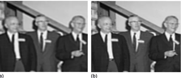
Fig. 5. The restored images at iteration 1 (a) (relative error = 1.14×10−1) and iteration 6 (b) (relative error = 8.97×10−2).

present the restored images at iterations 1 and 6. We see from Fig. 5 that the cigarette in Prof. Householder’s hand is better restored at iteration 6 than that at iteration 1. These preliminary numerical results show that our iterative scheme converges very fast. We plan to investigate the convergence of the iterative scheme.

In summary, we have presented a new approach image restoration by using regu-larized, constrained TLS image methods, with Neumann boundary conditions. Pre-liminary numerical results indicate the effectiveness of the method. Future work on this project will exploit the constrained TLS technique in phase diversity-based de-convolution arising from astronomy, extending work by Vogel et al. [34].

References

[1] H. Andrews, B. Hunt, Digital Image Restoration, Prentice-Hall, Englewood Cliffs, NJ, 1977. [2] M. Banham, A. Katsaggelos, Digital image restoration, IEEE Signal Processing Magazine, March

(21)

[3] T. Bell, Electronics and the stars, IEEE Spectrum 32 (8) (1995) 16–24.

[4] K. Castleman, Digital Image Processing, Prentice-Hall, Englewood Cliffs, NJ, 1996.

[5] R. Chan, M. Ng, Conjugate gradient methods for Toeplitz systems, SIAM Rev. 38 (1996) 427–482. [6] R. Chan, M. Ng, R. Plemmons, Generalization of Strang’s preconditioner with applications to

Toep-litz least squares problems, J. Numer. Linear Algebra Appl. 3 (1996) 45–64.

[7] T. Chan, C. Wong, Total variation blind deconvolution, IEEE Trans. Image Process. 7 (3) (1998) 370–375.

[8] J. Dennis, R. Schnabel, Numerical Methods for Unconstrained Optimalization and Nonlinear Equa-tion, Prentice-Hall, Englewood Cliffs, NJ, 1983.

[9] H. Engl, M. Hanke, A. Neubauer, Regularization of Inverse Problems, Kluwer Academic Publishers, The Netherlands, 1996.

[10] G. Golub, P. Hansen, D. O’Leary, Tikhonov regularization and total least squares, SCCM Research Report, Stanford, 1998.

[11] G. Golub, C. Van Loan, An analysis of total least squares problems, SIAM J. Numer. Anal. 17 (1980) 883–893.

[12] R. Gonzalez, R. Woods, Digital Image Processing, Addison-Wesley, New York, 1992.

[13] M. Hanke, J. Nagy, Restoration of atmospherically blurred images by symmetric indefinite conjugate gradient techniques, Inverse Problems 12 (1996) 157–173.

[14] J. Hardy, Adaptive Optics for Astronomical Telescopes, Oxford Press, New York, 1998. [15] S. Van Huffel, J. Vandewalle, The Total Least Squares Problem, SIAM, Philadelphia, PA, 1991. [16] A. Jain, Fundamentals of Digital Image Processing, Prentice-Hall, Englewood Cliffs, NJ, 1989. [17] S. Jefferies, J. Christou, Restoration of astronomical images by iterative blind deconvolution,

Astro-phys. J. 415 (1993) 862–874.

[18] J. Kamm, J. Nagy, A total least squares method for Toeplitz systems of equations, BIT 38 (1998) 560–582.

[19] T. Kelley, Iterative Methods for Optimization, SIAM, Philadelphia, PA, 1999.

[20] D. Kundur, D. Hatzinakos, Blind image deconvolution, IEEE Signal Processing Magazine, May 1996, pp. 43–64.

[21] R. Lagendijk, J. Biemond, Iterative Identification and Restoration of Images, Kluwer Academic Publishers, Dordrecht, 1991.

[22] R. Lagendijk, A. Tekalp, J. Biemond, Maximum likehood image and blur identification: a unifying approach, Opt. Eng. 29 (1990) 422–435.

[23] J. Lim, Two-Dimensional Signal and Image Processing, Prentice-Hall, Englewood Cliffs, NJ, 1990. [24] F. Luk, D. Vandevoorde, Reducing boundary distortion in image restoration, in: Proceedings of the SPIE 2296, Advanced Signal Processing Algorithms, Architectures and Implementations VI, 1994. [25] J. Nelson, Reinventing the telescope, Popular Sci. 85 (1995) 57–59.

[26] V. Mesarovi´c, N. Galatsanos, A. Katsaggelos, Regularized constrained total least squares image restoration, IEEE Trans. Image Process. 4 (1995) 1096–1108.

[27] S. Nash, A. Sofer, Linear and Nonlinear Programming, McGraw-Hill, New York, 1996.

[28] M. Ng, R. Chan, T. Wang, A fast algorithm for deblurring models with Neumann boundary condi-tions, Res. Rept. 99-04, Department of Mathematics, The Chinese University of Hong Kong; SIAM J. Sci. Comput. 21, 851–866.

[29] M. Ng, R. Plemmons, Fast recursive least squares using FFT-based conjugate gradient iterations, SIAM J. Sci. Comput. 17 (1996) 920–941.

[30] M. Ng, R. Plemmons, S. Qiao, Regularization of RIF blind image deconvolution, IEEE Trans. Image Process., June 2000, to appear.

[31] K. Rao, P. Yip, Discrete Cosine Transform: Algorithms, Advantages, Applications, Academic Press, Boston, MA, 1990.

(22)

[34] C. Vogel, T. Chan, R. Plemmons, Fast algorithms for phase diversity-based blind deconvolution, in: D. Bonaccini, R. Tyson (Eds.), Adaptive Optical System Technologies, Proceedings of SPIE, vol. 3353, 1998, pp. 994–105.

[35] Y. You, M. Kaveh, A regularization approach to joint blur identification and image restoration, IEEE Trans. Image Process. 5 (1996) 416–427.

[36] W. Zhu, Y. Wang, Y. Yao, J. Chang, H. Graber, R. Barbour, Iterative total least squares image recon-struction algorithm for optical tomography by the conjugate gradient algorithm, J. Opt. Soc. Amer. A 14 (1997) 799–807.