A new least-squares approach to differintegration modeling

Signal Processing 86 (2006) 2582–2591

A new least-squares approach to differintegration modeling

Manuel D. Ortigueira

_{, Anto´nio J. Serralheiro}

a_{UNINOVA and DEE, Faculdade de Cieˆncias e Tecnologia da Universidade Nova de Lisboa, Campus da FCT da UNL,} Quinta da Torre, 2829-516 Caparica, Portugal

b_{INESC ID, Rua Alves Redol, 9, 2}o_{, 1000-029 Lisboa, Portugal} c_{Academia Militar and CINAMIL, Rua Gomes Freire, 1150-175 Lisboa, Portugal} Received 20 May 2005; received in revised form 25 October 2005; accepted 14 December 2005

Available online 15 March 2006

Abstract

In this paper a new least-squares (LS) approach is used to model the discrete-time fractional differintegrator. This approach is based on a mismatch error between the required response and the one obtained by the difference equation defining the auto-regressive, moving-average (ARMA) model. In minimizing the error power we obtain a set of suitable normal equations that allow us to obtain the ARMA parameters. This new LS is then applied to the same examples as in [R.S. Barbosa, J.A. Tenreiro Machado, I.M. Ferreira, Least-squares design of digital fractional-order operators, FDA’2004 First IFAC Workshop on Fractional Differentiation and Its Applications, Bordeaux, France, July 19–21, 2004, P. Ostalczyk, Fundamental properties of the fractional-order discrete-time integrator, Signal Processing 83 (2003) 2367–2376] so performance comparisons can be drawn. Simulation results show that both magnitude frequency responses are essentially identical. Concerning the modeling stability, both algorithms present similar limitations, although for different ARMA model orders.

r2006 Elsevier B.V. All rights reserved.

Keywords: Discrete-time fractional differintegrator; Pseudo-fractional ARMA; Gru¨nwald–Letnikov derivative; Tustin bilinear transformation

1. Introduction

Fractional linear systems are described by frac-tional differential equations in the continuous-time case or ARMA models in the discrete-time case. The first case uses the definition of fractional derivative

[1]; the second uses the fractional differencing [2]. The long memory exhibited by these systems cannot be explained by the usual integer order pole/zero models. The basic building block of this kind of systems is the non-integer order derivative that has been approximated by fractional powers of the backward difference or the bilinear transformations (the former is exactly the building block of the fractional differencing). These approximations are IIR systems with non-rational transfer functions. However, these more correct models are difficult to implement and model in practice. For them, ARMA models are only approximations that we

www.elsevier.com/locate/sigpro

0165-1684/$ - see front matterr2006 Elsevier B.V. All rights reserved. doi:10.1016/j.sigpro.2006.02.013

_{Corresponding author. UNINOVA and DEE, Faculdade de} Cieˆncias e Tecnologia da Universidade Nova de Lisboa, Campus da FCT da UNL, Quinta da Torre, 2829-516 Caparica, Portugal. Tel.: +351 21 2948520; fax: +351 21 2957786.

E-mail addresses:mdortigueira@uninova.pt, mdo@dee.fct.unl.pt (M.D. Ortigueira),

call pseudo-fractional ARMA models[3]. In the last few years, a lot of attempts to obtain such models have been done (see [4–9]). However, it remains to clarify two important questions: (a) how to perform such modeling and (b) how to choose the most suitable orders. In impulse response modeling the well-known Pade´ algorithm is frequently used[2]. In

[3], we presented a suitable recursive algorithm for this modeling. Here, we will propose a different algorithm based on a least-squares (LS) criterion different from [4]. This algorithm defines a mis-match error between the required response and the one obtained by the difference equation defining the ARMA model. In minimizing the error power we obtain suitable normal equations that allow us to obtain the ARMA parameters. The algorithm is described in Section 2 where we compare it with the algorithm described in [3] through some current modeling examples.

2. Least-squares ARMA approximation

2.1. The discrete-time fractional differintegrator

The differintegrator is a continuous-time linear system with transfer function given, in the causal case, by

FðsÞ ¼sa (1)

for ReðsÞ4_{0[10]. To obtain discrete-time}

differinte-grators, we replace the variablesin (1) by a suitable rational function of z1_{. The most commonly}

used are:

(a) the backward difference, leading to a solution that is essentially the discretization of the Gru¨nwald–Letnikov derivative;

(b) the Tustin bilinear transformation.

Let the transfer function of these two fractional discrete-time systems be given, respectively, by

ðaÞHbdðzÞ ¼

1z1 T

a

; jzj4_{1 (2)}

and

ðbÞHbilðzÞ ¼

2

T

1z1

1þz1

a

; jzj4_{1. (3)}

Fractional differentiators and integrators are ob-tained, respectively, witha4_{0 and}ao0.

The computation of the inverse Z-transform of (2) is simple using the binomial series expansion:

hbdðnÞ ¼

1

Ta

a

n

ð1Þnun¼

1

Ta

ða_Þ

n

n! un, (4)

whereun is the discrete-time Heaviside function and

ðaÞ_n ¼aðaþ1Þ. . .ðaþn1Þ is the Pochhammer symbol.

Considering (3), it can be seen that the correspond-ing impulse response is actually a convolution of two binomial sequences corresponding to the numerator and the denominator. It is not difficult to obtain

hbilðnÞ

2

T

a Xn

k¼0

ða_Þ

k

k!

ð1Þnkða_Þ

nk

ðnkÞ! .

As

n!¼ ð1ÞkðnÞ_kðnkÞ! kpn (5) and

ðaÞ_n ¼ ð1Þkðanþ1Þ_kðaÞ_nk (6) we obtain

hbilðnÞ

¼ 2

T

a

ð1Þnða_Þ

n

n! Xn

k¼0

ða_Þ

kðnÞk

ða_nþ1Þk ð1Þk

k!

¼ 2

T

a

ð1Þnða_Þn

n! 2F1ða;n;anþ1;1Þ, ð7Þ

where 2F1(a,b;c,1) is the Gauss hypergeometric function that, for these arguments, does not have a closed form. (Prof. Volker Strehl, in a personal communication, stated that, almost surely,

2F1(a,n;an+1;1) satisfies a second order recursion formula.)

2.2. The algorithm

Both discrete-time representations are IIR sys-tems, but are not described by finite orders ARMA models. However, we intend to find approximations using finite orders ARMA models. There have been a lot of attempts to do it[4–6,8]. Here we propose a new LS identification algorithm different from that one proposed in[4].

will consider only these cases. The approximation we are looking for may be stated as

HðzÞ ¼ P1

m¼0fmzm

P1

n¼0gnzn

PM

m¼0bmzm

PN

n¼0anzn

. (8)

It is not difficult to see that we are dealing with an indeterminate problem, and we are going to propose an easy way to overcome it. Let (8) be written as

XN

n¼0 anzn

X1

m¼0

f_mzmX

M

m¼0 bmzm

X1

n¼0

g_nzn (9)

and make an inverse Z-transform to obtain

XN

n¼0

aifni

XM

i¼0

bigni; n2Zþ. (10)

This relation suggests us to define an error sequence by

en¼

XN

n¼0

aifni

XM

i¼0

bigni; n2Zþ. (11)

Let us assume that we haveLvalues of the impulse response we want to model. The error energy is given by

E¼X

L1

n¼0

e2_n¼X

L1

n¼0

XN

n¼0

aifni

XM

i¼0 bigni

" #2

. (12)

Let a0¼1. We are now going to compute the

unknown parameters through the derivatives ofEin order to the ARMA parameters. This procedure is similar to that used in[11]. Therefore, we obtain the following sets of normal equations:

XL1

n¼0

XN

i¼0

aifnifnk

XM

i¼0

bignifnk

" #

¼0,

k¼1;2;. . .;N ð13Þ

and

XL1

n¼0

X

N

i¼0

aifnignkþ

XM

i¼0

bignignk

" #

¼0,

k¼0;1;2;. . .;M. ð14Þ

Introducing the covariance matrices:

Rffðk;iÞ ¼

X

L1

n¼0

f_nif_nk, (15)

Rgfðk;iÞ ¼

X

L1

n¼0

g_nif_nk, (16)

Rggðk;iÞ ¼

XL1

n¼0

g_nig_nk (17)

we can rewrite (13) and (14) as

XN

i¼0

aiRffðk;iÞ

XM

i¼0

biRgfðk;iÞ ¼0; k¼1;2;. . .;N

(18)

and

XN

i¼0

aiRfgðk;iÞ

XM

i¼0

biRggðk;iÞ ¼0,

k¼0;1;2;. . .;N. ð19Þ If we know all the impulse response values or the theoretical expressions, we can compute the correla-tions

RffðkiÞ ¼

X1

n¼0

f_nf_nþik, (20)

RgfðkiÞ ¼

X1

n¼0

g_nf_nþik, (21)

RggðkiÞ ¼

X1

n¼0

g_ng_nþik (22)

that allow us to rewrite (18) and (19) as

XN

i¼0

aiRffðkiÞ

XM

i¼0

biRgfðkiÞ ¼0,

k¼1;2;. . .;N ð23Þ

and

XN

i¼0

aiRfgðkiÞ

XM

i¼0

biRggðkiÞ ¼0,

k¼0;1;2;. . .;N. ð24Þ With this formulation all the involved matrices are Toeplitz matrices. However, we will maintain the notation introduced in (18) and (19). We can join all the matrices in only one. Introduce the matrices

U_{½ðNþ1Þ ðNþ1Þ;}W_{½ðMþ1Þ ðNþ1Þ and} H_{½ðMþ1Þ ðMþ1Þ that are easily identified and}

aNb0b1b2. . .bMT: We join (18) and (19) into the

following system of equations:

U W

WT H

2 6 4 3 7 5 1 a1 .. . aN b0 .. . bM 2 6 6 6 6 6 6 6 6 6 6 6 6 6 4 3 7 7 7 7 7 7 7 7 7 7 7 7 7 5 ¼ Emin 0 : : : 0 2 6 6 6 6 6 6 6 6 6 6 6 6 6 4 3 7 7 7 7 7 7 7 7 7 7 7 7 7 5 . (25)

The solution is readily obtained by inverting the matrix. We only have to obtain the first column of the inverse and normalize the first coefficient. The normalizing constant is equal to Emin. The parti-tioned inverses formula can be used here [12]. To our needs it is enough to say that the first column of the following matrix is the solution (non-normal-ized) for our problem:

Emin 1 a1 .. . aN b0 .. . bM 2 6 6 6 6 6 6 6 6 6 6 6 6 6 4 3 7 7 7 7 7 7 7 7 7 7 7 7 7 5 ¼

ðUWH1WT_Þ1

WH1WT_ðUWH1WT_Þ1

2 6 4 3 7 5 1 0 : : : 0 2 6 6 6 6 6 6 6 6 6 6 6 6 6 4 3 7 7 7 7 7 7 7 7 7 7 7 7 7 5 (26)

provided that either ðUWH1WT_{Þ or} H _are

regular. If this is not the case, we can use

Emin 1 a1 .. . aN b0 .. . bM 2 6 6 6 6 6 6 6 6 6 6 6 6 6 6 6 6 4 3 7 7 7 7 7 7 7 7 7 7 7 7 7 7 7 7 5 ¼

ðU1_þU1W_ðHWTU1W_Þ1WTU1

ðHWTU1W_Þ1WTU1

2 6 6 4 3 7 7 5 1 0 : : : 0 2 6 6 6 6 6 6 6 6 6 6 6 6 6 6 6 6 6 4 3 7 7 7 7 7 7 7 7 7 7 7 7 7 7 7 7 7 5 . ð27Þ

We remark here thata0¼1 and thus

XN

i¼1

aiRffðkiÞ

XM

i¼0

biRgfðkiÞ

" #

¼ RffðkÞ,

k¼1;2;. . .;N ð28Þ

and

XN

i¼1

aiRfgðkiÞ

XM

i¼0

biRggðkiÞ

" #

¼ RfgðkÞ,

k¼0;1;2;. . .;M. ð29Þ

This may be interesting because it allows a reduction in the dimensions of matrices U _and W_.

It is not difficult to obtain similar matrices to those in (25)–(27).

2.3. Applications

2.3.1. Difference

We are going to use the previous algorithm to compute the approximation to the differintegrator using the backward difference. Assume thata4_{0. In}

this case and referring to the notation used in the previous section, we have

f_n¼ 1

Ta

ða_Þ

n

n! un (30)

and

gn ¼dn. (31)

Let the corresponding correlations be computed:

RffðnÞ ¼

1

T2a

X1

k¼0

a

k

!

ð1Þk a

kþn

!

ð1Þkþn

¼ 1

T2a

X1

k¼0

ða_Þk

k!

As

ðnþkÞ!¼ ðnþ1Þ_kn! (32)

and

ða_Þ

nþk¼ ðaÞnðaþnÞk, (33)

1

T2a

ða_Þ

n

n! X1

k¼0

ða_Þ

k

k!

ða_þnÞ

k

ðnþ1Þ! 1

T2a

ða_Þ

n

n! 2F1ða;aþn;nþ1;1Þ. ð34Þ

Using the Gauss formula

2F1ða;b;c;1Þ ¼

G_ðcÞG_ðcabÞ

G_ðcaÞG_ðcbÞ cab40 (35)

we obtain

RffðkÞ ¼

1

T2að1Þ

k Gð1þ2aÞ

G_ða_þkþ1ÞG_ða_kþ1Þ (36) meaning that theF_{matrix is a symmetric Toeplitz} matrix. Obviously

RgfðnÞ ¼

1

Ta

a

n

ð1Þnun. (37)

Then, C _{is a non-symmetric Toeplitz matrix. If} ao0, it is enough to interchangef_n withg_n.

2.3.2. Bilinear

Assume again thata4_{0. For thef}

n sequence, we

use the above expression (30). Forg_n we have

g_n¼ a

n

un. (38)

The corresponding autocorrelation is

RggðkÞ ¼

G_ð1þ2a_Þ

Gðaþkþ1ÞGðakþ1Þ (39)

leading again to a symmetric Toeplitz matrix. The cross-correlation is given forn4_{0 and}ao1

RfgðnÞ ¼

1

Ta

X1

k¼0

a

k

!

ð1Þk a

kþn

!

¼ 1

Ta

X1

k¼0

ða_Þk

k! ða_Þ

kþn

ðkþnÞ!

¼ 1

Ta

ða_Þ

n

n! X1

k¼0

ða_Þ

kðaþnÞk

ð1þnÞ_k

¼ 1

Ta

ða_Þ

n

n! 2F1ðaþn;a;nþ1;1Þ.

From Kummer’s formula[13]

2F1ða;b;abþ1;1Þ ¼

Gð1þabÞGð1þa=2Þ

Gð1þa=2bÞGðaþ1Þ,

bo1 and ab nonnegative integer

ð40Þ

we obtain

RfgðnÞ ¼

1

Ta

ða_Þ

n

n!

G_ð1a_þnÞG_ð1a_=2þn=2Þ G_ð1þa_=2þn=2ÞG_ða_þnþ1Þ

¼ 1

Ta

ð1Þn G_ða_Þða_þnÞ

G_ð1a_=2þn=2Þ G_ð1þa_=2þn=2Þ.

ð41Þ

Ifno0

RfgðnÞ ¼ ð1ÞnRfgðnÞ (42)

leading to a non-symmetric Toeplitz matrix. In this case and if N¼M, we have

bi¼ ð1Þiai

suggesting the usage of an ARMA(N,N).

3. Comparisons

In this section we are going to use the above algorithm to compute approximations for the differintegrator. However, only the results for the differentiator (a4_{0) are presented since, for}

prac-tical purposes, the integrator does not constitute a different case study. This leads us to consider fractional orders a_{2 ½0:5;0:5. For comparisons,} we will use the results presented in [3,4] whenever feasible.1

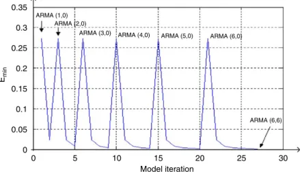
In order to get some insight into the order of the ARMA models, experiments with ARMA(n,m),n¼ 1;. . .;N and m¼0;. . .;n were performed. Figs. 1 and 2depict the behavior ofEmin, for the backwards difference and bilinear, respectively, as by Eq. (26) as a function of (n,m). It is interesting to note that in both cases, the local minima of Emin occur when

n¼m, that is, the number of poles equals the number of zeros. Also note that maxima correspond to AR(N) models.

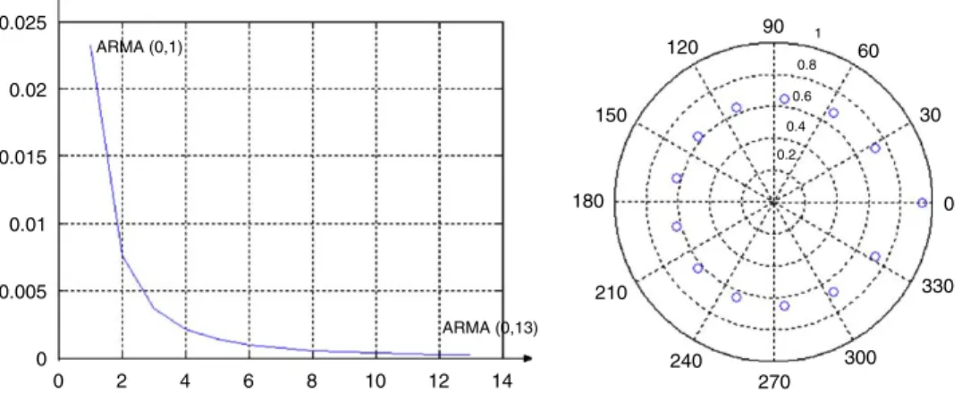
Further simulations were carried out for both the backward differences and bilinear MA(M) models.

Fig. 3 (backward differences) and Fig. 4 (bilinear) depictEminas a function of model order (left graph) and the final zero map (right graph).

Based on the Emin behavior as a function of the order of the models, all the remaining experiments comprise only ARMA(N,N) models.

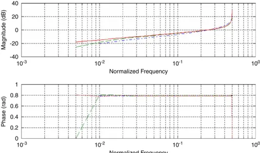
AsFigs. 5 and 6depict, there is no substantial or significant difference between the algorithm pro-posed in this work, LS, and that presented in[3].

In the LS case, higher ARMA orders can be thought but, for comparison purposes with the previous algorithm, we limited them to (9,9). In fact, using the LS approach, and for a_{¼0:5, we were} able to estimate an ARMA(12,12), depicted in

Fig. 7. It should be pointed out that, for this same value ofa_{¼0:5, in[3]instability problems occurred} forðN;NÞ4_9.

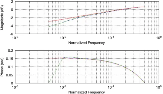
Changing the value ofa _{to 0.1 leads us toFig. 8} (backward differences) and Fig. 9(bilinear). These approximations are summarized inTable 1.

Values of ja_j4_{0:5 are not interesting to present}

since they can be trivially reduced to a ‘‘new’’ fractional order a_{¼ ð1aÞ such that a 2 ½0;0:5} by including either an integrator or a differenciator that results in an extra ð1z1_Þ1 _{or ð1z}1_Þ

factor, respectively. This extra factor can have adverse effects in control applications, specially if it results as an integrator. In this case,a _{should be} restricted to [0, 1], instead.

Unfortunately, no definitive assertions can be made on the order of the ARMA models since no Emin

0.35

0.3

0.2

0.1

0 0

5 10 15 20 25 30 0.25

0.15

0.05

Model iteration

ARMA (6,6) ARMA (6,0)

ARMA (5,0) ARMA (4,0)

ARMA (3,0) ARMA (2,0) ARMA (1,0)

Fig. 1. Eminas a function of model order fora¼0:5 and backward differences. Local minima correspond to ARMA(n,n) and the last sample being for ARMA(6,6).

Emin 0.9

0.8

0.6

0.4

0

0 10 20 30 40 50 60 70 80 90 0.7

0.5

0.3

0.2

0.1

Model iteration ARMA (9,9)

ARMA (12,12) ARMA (12,0) ARMA (11,0)

ARMA (2,0) ARMA (1,0)

0.02

0

0 2 4 6 8 10 12 14

1 0.8 0.6 0.4 0.2

0.025

0.015

0.01

0.005

ARMA (0,13) ARMA (0,1)

90

60

30

0

330

300 270 240 210 180

150 120

Fig. 3. Emin(left plot) for ARMA(0,m), m¼1;. . .;13 and zeros on thez-plane for ARMA(0,13) (right plot) both fora¼0:5 and backward differences.

0.2

0

0 2 4 6 8 10 12 14

1

0.8

0.6

0.4

0.2 0.25

0.15

0.1

0.05

ARMA (0,13)

ARMA (0,1) 90

60

30

0

330

300 270 240

210 180

150 120

Fig. 4.Emin(left plot) for ARMA(0,m),m¼1;. . .;13 and zeros on thez-plane for ARMA(0,13) (right plot) both fora¼0:5 and bilinear.

10

0

-10

-30 -20

0.8

0.6

0.4

0.2

0

Phase (r

ad)

Magnitude (dB)

10-3 ₁₀-2 ₁₀-1 ₁₀0

Normalized Frequency

10-3 ₁₀-2 ₁₀-1 ₁₀0

Normalized Frequency

further evidence was drawn from the simulations we performed. However, the bilinear seems to be more stable than the backward differences, and this behavior appears to be valid for values ofa_{2 f0:1;0:5;0:8g. As}

a final note, and for the presented examples (regardless the value ofa_{and the chosen approximation), all the} poles and zeros were real-valued as long as models remain ARMA(N,N).

40

20

0

-40 -20

0.8 1

0.6

0.4

0.2

0

Phase (r

ad)

Magnitude (dB)

10-3 ₁₀-2 ₁₀-1 ₁₀0

Normalized Frequency

10-3 10-2 10-1 100

Normalized Frequency

Fig. 6. ARMA(9,9) amplitude (top, in dB) and phase (bottom, in radians) frequency response plots for the bilinear, witha¼0:5. LS approach is the solid line, the exact model spectrum is the dash-dotted line, while as in[7]is the dashed line.

40

20

0

-40 -20

0.8 1

0.6

0.4

0.2

0

Phase (r

ad)

Magnitude (dB)

10-3 ₁₀-2 ₁₀-1 ₁₀0

Normalized Frequency

10-3 10-2 10-1 100

Normalized Frequency

4. Conclusions

We proposed here a new LS algorithm for pole–zero modeling of fractional linear systems. This is based on an error power minimization relatively to the ARMA models that leads to a set of

normal equations. We applied to two well-known situations consisting of the difference and bilinear transformations that are suitable for exact auto-correlation computation. Some illustrating exam-ples were presented showing that ARMA(N,N) are suitable models.

2

0

-2

-6 -4

0.15 0.2

0.1

0.05

0

Phase (r

ad)

Magnitude (dB)

10-3 ₁₀-2 ₁₀-1 ₁₀0

Normalized Frequency

10-3 10-2 10-1 100

Normalized Frequency

Fig. 8. ARMA(6,6) amplitude (top, in dB) and phase (bottom, in radians) frequency response plots for the backward difference, with a¼0:1. LS approach is the solid line, the exact model spectrum is the dash-dotted line, while as in[2]is the dashed line.

10

5

0

-10 -5

0.15 0.2

0.1

0.05

0

Phase (r

ad)

Magnitude (dB)

10-3 ₁₀-2 ₁₀-1 ₁₀0

Normalized Frequency

10-3 ₁₀-2 ₁₀-1 ₁₀0

Normalized Frequency

References

[1] M.D. Ortigueira, ARMA realization from the reflection coefficient sequence, Signal Processing 32 (3) (June 1993). [2] M.D. Ortigueira, F.V.C. Coito, From differences to

differ-integrations, Fractional Calculus Appl. Anal. 7 (4) (2004). [3] M.D. Ortigueira, A.J.S. Serralheiro, Pseudo-fractional

ARMA modelling using a double Levinson recursion, IEE Proc. Control Theory Appl., accepted for publication. [4] R.S. Barbosa, J.A. Tenreiro Machado, I.M. Ferreira,

Least-squares design of digital fractional-order operators, FDA’2004 First IFAC Workshop on Fractional Differentiation and Its Applications, Bordeaux, France, July 19–21, 2004.

[5] R.S. Barbosa, J.A. Tenreiro Machado, I.M. Ferreira, Pole–zero approximations of digital fractional-order inte-grators and differentiators using signal modeling techniques, Proceedings of the 16th IFAC World Congress, Prague, Czech Republic, July 2005.

[6] Y.Q. Chen, B.M. Vinagre, A new IIR-type digital fractional order differentiator, Signal Processing 83 (2003) 2359–2365.

[7] P. Ostalczyk, Fundamental properties of the fractional-order discrete-time integrator, Signal Processing 83 (2003) 2367–2376.

[8] J.A. Tenreiro Machado, Discrete-time fractional-order controllers, Fractional Calculus Appl. Anal. J. 1 (2001) 47–66.

[9] B.M. Vinagre, I. Podlubny, A. Hernandez, V. Feliu, Some approximations of fractional order operators used in control theory and applications, Fractional Calculus Appl. Anal. 3 (3) (2000) 231–248.

[10] M.D. Ortigueira, J.A. Tenreiro-Machado, J. Sa´ da Costa, Which differintegration? IEE Proc. Vision Image Signal Process 152 (6) (2005) 846–850.

[11] K. Steiglitz, On the simultaneous estimation of poles and zeros in speech analysis, IEEE Trans. Acoust. Speech Signal Process. ASSP-25 (3) (June 1977).

[12] H. Lu¨tkepohl, Handbook of Matrices, Wiley, New York, 1996.

[13] P. Henrici, Applied and Computational Complex Analysis, vol. 2, Wiley, New York, 1991, pp. 389–319.

Table 1

Selected transfer functions for the LS approach

a ARMA Model AR coefficients MA coefficients

0.1 (6,6) Backward 1.0000;3.4875; 4.7052;3.0595; 0.9645;0.1269; 0.0041

1.0000;3.5875; 5.0090;3.4016; 1.1375;0.1638; 0.0064

0.1 (12,12) Bilinear 1.0000; 0.0997;3.3770;0.3037; 4.3668; 0.3438;2.67560.1753; 0.7699; 0.0381;0.0857;0.0025; 0.0017

1.0000; 0.1003;3.3770; 0.3057 4.3666;

0.3460;2.6755; 0.1765; 0.7699;

0.0383;0.0857; 0.0025; 0.0017 0.5 (6,6) Backward 1.0000;3.2112; 3.9246;2.2548;

0.6019;0.0612; 0.0011

1.0000;3.7112; 5.4052;3.8782; 1.4004;0.2274; 0.0113

0.5 (9,9) Bilinear 1.0000; 0.5000;2.30191.0260; 1.7917; 0.6706;0.5282;0.1450; 0.0437; 0.0052

1.0000;0.5000;2.3019; 1.0260; 1.7917;0.6706;0.5282; 0.1450; 0.04370.0052

0.5 (12,12) Bilinear 1.0000; 0.5001;3.1883;1.4696; 3.8645; 1.5967;2.1989;0.7768; 0.5801; 0.1596;0.0581;0.0097; 0.0010