Mesonic eightfold way from dynamics and confinement in strongly coupled lattice quantum chromodynamics

Mesonic eightfold way from dynamics and confinement

in strongly coupled lattice quantum chromodynamics

Antônio Francisco Neto,1,a兲 Michael O’Carroll,2and Paulo A. Faria da Veiga2,b兲

1

Campus Alto Paraopeba, UFSJ, CP 131, 36.420–000 Ouro Branco MG, Brazil 2

Departamento de Matemática Aplicada e Estatística, ICMC-USP, CP 668, 13560-970 São Carlos SP, Brazil

共Received 20 November 2007; accepted 9 March 2008; published online 3 July 2008兲

We show the existence of all the 36 eightfold way mesons and determine their masses and dispersion curves exactly, from dynamical first principles such as di-rectly from the quark-fluon dynamics. We also give a proof of confinement below the two-meson energy threshold. For this purpose, we consider an imaginary time functional integral representation of a 3⫹1 dimensional lattice QCD model with Wilson action, SU共3兲f global and SU共3兲clocal symmetries. We work in the strong coupling regime, such that the hopping parameter␬⬎0 is small and much larger than the plaquette coupling ␤⬎1/g₀2艌0 共␤Ⰶ␬Ⰶ1兲. In the quantum mechanical physical Hilbert spaceH, a Feynman-Kac type representation for the two-meson correlation and its spectral representation are used to establish an exact rigorous connection between the complex momentum singularities of the two-meson trun-cated correlation and the energy-momentum spectrum of the model. The total spin operator J and its z-component Jz are defined by using ␲/2 rotations about the spatial coordinate axes, and agree with the infinitesimal generators of the con-tinuum for improper zero-momentum meson states. The mesons admit a labelling in terms of the quantum numbers of total isospinI, the third componentI3of total isospin, thez-componentJzof total spin and quadratic CasimirC2for SU共3兲f. With this labelling, the mesons can be organized into two sets of states, distinguished by the total spinJ. These two sets are identified with the SU共3兲fnonet of pseudo-scalar mesons(J= 0兲and the three nonets of vector mesons共J= 1 ,Jz=⫾1 , 0兲. Within each nonet a further decomposition can be made using C2 to obtain the singlet state 共C2= 0兲 and the eight members of the octet 共C2= 3兲. By casting the problem of determination of the meson masses and dispersion curves into the framework of the the anaytic implicit function theorem, all the massesm共␬,␤兲are found exactly and are given by convergent expansions in the parameters␬ and␤. The masses are all of the formm共␬,␤= 0兲⬅m共␬兲= −2ln␬− 3␬2_{/2 +␬}4_{r共␬兲withr共0兲⫽0 andr共␬兲real} analytic; for␤⬎0 ,m共␬,␤兲+ 2ln␬is jointly analytic in␬and␤. The masses of the vector mesons are independent ofJ_zand are all equal within each octet. All isospin singlet masses are also equal for the vector mesons. For each nonet and␤= 0, up to and includingO共␬4_{兲, the masses of the octet and the singlet are found to be equal.} But there is a pseudoscalar-vector meson mass splitting given by 2␬4_+O共␬6_兲and the splitting persists for␤⬎0. For␤= 0, the dispersion curves are all of the form

w共pជ兲= −2 ln␬− 3␬2_/

2 +

共

1₄

兲

␬2_兺 j=1 3

2共1 − cospj兲+␬4_r共␬

,pជ兲, with兩r共␬,pជ兲兩艋const. For the pseudoscalar mesons,r共␬,pជ兲is jointly analytic in␬ andpj_{, for兩␬兩 and兩Imp}j_兩

a兲_{Electronic mail: afneto@fisica.ufs.br.} b兲_{Electronic mail: veiga@icmc.usp.br.}

49, 072301-1

small. We use some machinery from constructive field theory, such as the decou-pling of hyperplane method, in order to reveal the gauge-invariant eightfold way meson states and a correlation subtraction method to extend our spectral results to

allHe, the subspace ofHgenerated by vectors with an even number of Grassmann

variables, up to near the two-meson energy threshold of⬇−4 ln␬. Combining this result with a previously similar result for the baryon sector of the eightfold way, we show that the only spectrum in allH⬅He丣Ho共Ho_{being the odd subspace}兲_below ⬇−4 ln␬ is given by the eightfold way mesons and baryons. Hence, we prove confinement up to near this energy threshold. © 2008 American Institute of Physics. 关DOI:10.1063/1.2903751兴

I. INTRODUCTION

A landmark in particle physics was achieved when Gell-Mann and Ne’eman independently proposed the eightfold way scheme to classify the then known hadronic particles共see Refs.1–5兲. This model asserts that every hadron is composed of quarks with three flavors—up共u兲,down共d兲, and strange 共s兲. The baryons are made of three quarks and the mesons are made of a quark-antiquark pair. Later, a color dynamics was introduced for the quarks via an exchange of gauge vector bosons called gluons, and today the local gauge model of interacting quarks and gluons based on the color symmetry SU共3兲c, which is known as the quantum chromodynamics共QCD兲, is the best candidate to describe the strong interactions.

The lattice regularization of the continuum theory was introduced by Wilson in Ref.6. Pre-cisely, in Ref.6, an imaginary-time functional integral formulation for lattice QCD was developed. In this framework, there are basically two ingredients: quarks, obeying Fermi–Dirac statistics, carrying flavor, color and spin labels, and located in each lattice site, and colored string bits connecting adjacent points on the lattice. Besides preserving gauge invariance and being free of ultraviolet singularities, the lattice formulation is powerful enough to, e.g., obtain the first results on the QCD particle spectrum and to exhibit confinement, i.e., isolated quarks are not observed. Within this construction, one formally recovers the continuum theory in the scaling limit共i.e., the lattice spacing going to zero兲. Later, it was shown by Osterwalder and Seiler that the lattice regularization of Wilson has the property of reflection positivity 共see Refs. 7 and 8 for more details兲. This property enables the construction of the quantum mechanical Hilbert space of physi-cal states H and allows us to define a positive self-adjoint energy and self-adjoint momentum operators. Within this framework, a Feynman–Kac 共FK兲 formula is established and the energy-momentum共E-M兲spectrum can be investigated.

We point out that even for ␤= 0共no plaquette terms in the action兲, there is still a nontrivial dependence on the gauge field in the quadratic Fermi field hopping term. One manifestation of this dependence is that the meson dispersion curves have a small momentum behavior approximately proportional to␬2_pជ2_{. For free fermions 共such as setting the gauge group elements equal to the} identity兲, the behavior is proportional to␬pជ2 _{and the free fermion mass is asymptotically −ln␬.}

The baryons are detected as complex momentum singularities of the Fourier transform of a two-baryon correlation and are rigorously related to theE-M spectrum via a spectral representa-tion to this quantity. The spectral representarepresenta-tion for the two-point correlarepresenta-tion is derived by using a FK formula.

The 56 baryon states can be grouped into two octets of total spin J=1₂

共J

z=⫾ 1

2

兲

and four decuplets of total spinJ=3₂

共J

z=⫾₂1,⫾3₂

兲

. On the lattice, there is only the discrete␲/2-rotation group. However, we can adapt the treatment usually employed in solid state physics and use the structure of point groups 共see Ref. 23兲 to rigorously introduce total spin operators J and spin

z-component Jz so that for zero-momentum states, there is a partial restoration of rotational symmetry, which means that these operators inherit the same structure as for the continuum. Using this shows that the masses within the octets and within the decuplets are independent of Jz. However, there is a mass splitting between the octets and the decuplets given to leading order of 3␬6_/

4 at␤= 0. For␤⫽0 andmb共␬兲as the baryon mass,mb共␬兲+ 3 ln␬is jointly analytic in␬and ␤. In particular, the mass splitting between octet and decuplet persists for ␤⫽0.

It is worth remarking that the work of Refs. 20 and 21 is not the first publication on the one-particle spectrum of lattice QCD models with three flavors. Specially in the 1980s, many papers were devoted to the existence of baryons, e.g., the work of Refs.24and25. However, these papers do not rely on spectral representations. This can be problematic when tiny splitting among the states is present. Also, the determination of momentum singularities of the two-point function via the zeros of uncontrolled expansion in the denominator of the Fourier transform of approxi-mate propagators leaves the question of the nature and the existence of the supposed singularity unanswered. The same kind of problems may show up in works where the masses are determined by the exponential decay rates of two-point functions, as what is usually done in numerical simulations. We remark that we work with the exact correlation function, its convolution inverse, and their Fourier transforms.

In this work, in the strong coupling regime, and using the decoupling of hyperplane method 共see Ref.26–29兲, we complete the exact determination of the one-particleE-Mspectrum initiated in Refs. 20 and 21. For a pedagogical presentation of the basic principles of the hyperplane decoupling method, see Ref. 28. Here, we consider the even subspace He傺H and show the existence of the 36 eightfold way meson共of asymptotic mass −2 ln␬兲states.

The hyperplane decoupling method has many nice features.

• It enables us to obtain the basic local gauge-invariant excitation fields without anya priori

guesswork. As will be shown, linear combination of these fields can be identified with the eightfold way particles, namely, the pseudoscalar and vector mesons.

• It gives good control of the global decay properties of the correlation functions involved. • It enables us to show that the spectrum is generated by isolated dispersion curves, i.e., the

upper gap property.

• It permits us to show that the only spectrum in all He is generated by the eightfold way particles.

The meson particles are detected by isolated dispersion curvesw共pជ兲in the energy-momentum spectrum. They are of the form, for ␤= 0, w共pជ兲= −2 ln␬− 3␬2_{/2 +}

共

1

4

兲

␬ 2_兺

j=1 3

2共1 − cospj_兲 +␬4_r共␬

,pជ兲with兩r共␬,pជ兲兩艋const. For the pseudoscalar mesons,r共␬,pជ兲is jointly analytic in␬and

pj_{, for兩␬兩 and兩Imp}j_{兩 small. The meson masses are given bym共␬兲= −2 ln␬− 3␬}2_{/2 +␬}4_{r共␬兲with}

r共0兲⫽0 andr共␬兲real analytic. The nonsingular part of the mass, i.e.,r共␬兲, is jointly analytic in␬ and␤. For a fixed nonet, the masses of all vector mesons are independent ofJzand are all equal within each octet. All singlet masses are also equal. For␤= 0, up to and includingO共␬4_{兲, for each} nonet, the masses of the octet and the singlet are found to be equal. All members of each octet have identical dispersions. Other dispersion curves may differ. Indeed, there is a pseudoscalar vector meson mass splitting共betweenJ= 0 andJ= 1兲given by 2␬4_+O共␬6_{兲and, by analyticity, the} splitting persists for␤⫽0. Using a correlation subtraction method, we show that the 36 meson states give the only spectrum inHeup to near the two-meson threshold of ⬇−4 ln␬. Up to and includingO共␬4_{兲, there is no isospin singlet-isospin octet mass splitting at␤= 0. There may be a} splitting at higher order in ␬ and ␤. For this splitting in the continuum model, see the U共1兲 problem in Ref.30.

Combining the present result with the results of Refs.20and21shows confinement up to the two-meson threshold. We stress that even within the limitation of dealing with only three quark flavors, since not all the eightfold way hadrons have not, up to now, been experimentally observed 共specially the heavy decuplet baryons and the scalar mesons兲, our results still give more strength to the Gell-Mann and Ne’eman quark model.

This paper is organized as follows. In Sec. II, we introduce the Wilson’s lattice QCD model that we use. The decoupling of hyperplane method is also used to reveal the form of the basic excitation fields in He. To establish a connection with the E-M spectrum, we define a matrix valued two-point meson functionG, in terms of the basic excitation fields with individual quark and antiquark spin and isospin labels, and introduce a spectral representation for G. Our main result, stating the existence of the eightfold way mesons, determining their masses, multiplici-tiesm, and dispersion curves, is then presented in Theorem 1. To determine the meson masses and dispersion curves, we analyze the convolution inverse⌳ of the two-point correlation. We need global bounds onGand⌳as well as their short distance behavior to the lowest orders in␬. They are given in Theorems 2 and 3, respectively. In Sec. III, we make a basis change from the individual spin and isospin basis to the particle basis. This basis change is implemented by an orthogonal transformation共normalized at␬= 0兲and allows us to identify the basic excitation fields with the eightfold way pseudoscalar and vector mesons. As for the baryon case, to carry out this identification, we label the states by their associated quantum numbers—total isospin I, its third componentI3, total hypercharge, and quadratic CasimirC2—by using the global flavor symmetry. We also need to consider spin and we adopt the same prescription as in Refs.20and21in such a way that for improper zero-momentum meson states, the total spin operatorJand related operators

Jx,Jy, andJz共and alsoJ⫾兲agree with the infinitesimal generators of the continuum. Finally, we

II. MODEL AND RESULTS

In the first subsection, we introduce the lattice QCD model and the physical quantum me-chanical Hilbert space H. In particular, the FK formula and the self-adjoint E-M operators are considered. We also state our main results on the E-M spectrum and the existence of meson particles in allHein Theorem 1. In the second subsection, the decoupling of hyperplane method is introduced and used to obtain the basic excitation states appearing in the two-point function. To determine the E-M spectrum, we need the long distance and short distance behaviors of the two-point function and its convolution inverse, which are presented in Theorems 2 and 3.

A. Model and the physical quantum mechanical Hilbert space

We use the same model presented in Refs.20 and21. The model is the SU共3兲f lattice QCD with the partition function formally given by Z=兰e−S共␺,␺¯,g兲d␺d␺¯ d␮共g兲, and for a function

F共␺,␺¯,g兲, the normalized correlations are denoted by

具F典=1

Z

冕

F共␺,␺

¯_,g兲e−S共␺,␺¯,g兲_{d␺d␺¯ d␮共g兲. 共1兲}

The actionS⬅S共␺,␺¯,g兲 is given by

S共␺,␺¯,g兲=␬ 2

兺

␺

¯

a,␣,f共u兲⌫␣␤⑀ e␳

U共gu,u+⑀e␳兲ab␺b,␤,f共u+⑀e␳兲+

兺

u_苸Z

o

4

␺

¯

a,␣,f共u兲M␣␤␺a,␤,f共u兲

− 1

g0 2

兺

p

␹共gp兲, 共2兲

where the first sum is overu苸Z

o 4

,⑀=⫾1 and␳= 0 , 1 , 2 , 3 and over repeated indices. By denoting 0 as the temporal direction, the lattice is given by Z

o 4

, where u=共u0,uជ兲=共u0,u1,u2,u3兲苸Z

o 4

⬅Z_1/2⫻Z3_{, whereZ}

1/2=

兵⫾

12,⫾ 3

2, . . .

其

. For each siteu苸Zo 4

, there are fermionic fields represented by Grassmann variables␺_a,␣,f共u兲, associated with a quark, and␺¯_a,␣,f共u兲, associated with an anti-quark, which carry a Dirac spin␣= 1 , 2 , 3 , 4, a colora= 1 , 2 , 3, and flavor or “isospin” f=u,d,s

= 1 , 2 , 3 index.⌫ is related to the Dirac matrices by ⌫⫾e␳

= −1⫾␥␳_{. The␥}␳ _{are the Dirac 4⫻4} matrices

␥0

=

冉

I2 0 0 −I2

冊

and␥j

=

冉

0 i␴ j

−i␴j 0

冊

, where␴j_{, j= 1 , 2 , 3, denote the Pauli 2⫻2 matrices and I}

2 is the 2⫻2 identity matrix. For each oriented bound on the lattice具u,u⫾e␳典, there is a matrixU共g_u,u⫾e␳兲苸SU共3兲parametrized by the gauge group elementU共gu,u⫾e␳兲satisfyingU共gu,u+e␳兲−1=U共gu+e␳,u兲. The parameter␬is the hopping parameter and␤⬅1/g₀2is the plaquette coupling. The measured␮共g兲is the product measure over nonoriented bonds of normalized SU共3兲cHaar measures共see Ref.32兲. There is only one integra-tion variable per bond, so that g_uv and gvu

−1

are not treated as distinct integration variables. The integrals over Grassmann fields are defined according to Ref.33. For a polynomial in the Grass-mann variables with coefficients depending on the gauge variables, the fermionic integral is defined as the coefficient of the monomial of maximum degree, i.e., of 兿u,k␺k共u兲␺¯k共u兲, k ⬅共a,␣,f兲. In Eq.共1兲,d␺d␺¯ means 兿u,kd␺k共u兲d␺¯k共u兲such that with a normalizationN=具1典, we have具␺k₁共x兲␺¯k₂共y兲典=共1/N兲兰␺k₁共x兲␺¯k₂共y兲e−兺u,k3,k4␺

¯

k₃共u兲Ok₃k₄␺k₄共u兲_d␺d␺¯_=O ␣₁␣₂ −1

ana-lytic functions in the global coupling parameters␬and␤⬅1/g₀2and also in any finite number of local coupling parameters. For the formal hopping parameter expansion, see Refs.34–36.

Associated with the SU共3兲f model, there is an underlying physical Hilbert space which we denote byH. Starting from gauge-invariant correlations with support restricted tou0=₂1and letting

T₀x0,T_ixi,i= 1 , 2 , 3, denoting translation of the functions of Grassmann and gauge variables共is used to denote Hilbert space operators兲byx0艌0,xជ=共x1,x2,x3兲苸Z3

, there is the FK formula forFand

Gonly depending on coordinates withu0₌1

2 given by

共G,Tˇ0 x0

Tˇ1 x1

Tˇ2 x2

Tˇ3 x3

F兲H=具关T0 x0

TជxជF兴⌰G典, 共3兲

whereTជxជ=T₁x1T₂x2T₃x3 and⌰is an antilinear operator that involves time reflection. Following Ref. 10, the action of⌰on single fields is given by

⌰␺¯a,␣,f共u兲=共␥0兲␣␤␺a,␤,f共ut兲,

⌰␺a,␣,f共u兲=␺¯a,␤,f共ut兲共␥0兲␤␣,

where u_t=共−u0_{,uជ兲 for A and B monomials, ⌰共AB兲=⌰共B兲⌰共A兲, and ⌰f共兵g}

uv其兲=f*共兵gu_tv

t其兲, u,v

苸Z_o4, for a function of the gauge fields whereⴱ_{means complex conjugate.⌰antilinearly extends}

to the algebra. For simplicity, we do not distinguish between Grassmann and gauge variables and their associated Hilbert space vectors in our notation. As linear operators inH,Tˇ_␳,␳= 0 , 1 , 2 , 3, are mutually commuting;Tˇ0is self-adjoint with −1艋Tˇ0艋1 andTˇj=1,2,3 are unitary. So, we writeTˇj =eiPj and Pជ=共P1,P2,P3兲 is the self-adjoint momentum operator with spectral points pជ苸T3

⬅共−␲,␲兴3_{. SinceTˇ} 0 2

艌0, the energy operatorH⬎0 can be defined byTˇ₀2=e−2H_{. We call a point in} theE-M spectrum associated with spatial momentumpជ= 0ជ a mass and, to be used below, we let E共␭0,␭ជ兲be the product of the spectral families ofTˇ0,P1,P2, andP3. By the spectral theorem共see Ref.37兲, we have

Tˇ₀=

冕

−␲

␲

␭0dE₀共␭0兲, Tˇ_j=1,2,3=

冕

−␲

␲

ei␭j_dF j共␭j兲,

so thatE共␭0,␭ជ兲=E0共␭0兲兿j=1 3 _F

j共␭j兲. The positivity condition具F⌰F典艌0 is established in Ref.8, but there may be nonzeroF’s such that 具F⌰F典= 0. If the collection of suchF’s is denoted byN, a pre-Hilbert spaceH

_⬘

can be constructed from the inner product 具G⌰F典and the physical Hilbert spaceHis the completion of the quotient spaceH

_⬘

/N, including also the Cartesian product of the inner space sectors, the color spaceC3

, the spin spaceC4

, and the isospin spaceC3 .

By considering the parameters␬,␤, it is to be understood that the following conditions hold in the sequel: there exist␬0⬎0,␤0⬎0, and␤0/␬0⬎0 sufficiently small. Under this condition, our results hold for all physical values of␬and␤such that␬⬍␬₀,␤⬍␤₀, and␤/␬艋␤₀/␬₀Ⰶ1. The main result of this paper is summarized in Theorem 1 below.

Theorem 1:The low-lying energy-momentum spectrum of the lattice QCD model given by the action of Eq.(2)in the strong coupling regime, in the even subspace He傺H,and up to near the

two-meson threshold of⬇−4 ln␬is generated by 36 states, which are bound states of a quark and an anti-quark. These 36 states are labelled by theSU共3兲fquantum numbers I,I3,Y,and C2.Also,

for zero-momentum states, a spin labeling can be introduced. The meson states can be distin-guished and grouped into threeSU共3兲fnonets associated with the vector mesons共J= 1,Jz= 0,⫾1兲

and one nonet associated with the pseudoscalar mesons 共J= 0兲. Each nonet admits a further decomposition into aSU共3兲f singlet共C2= 0兲 and an octet共C2= 3兲.The particles are detected by

w共pជ兲= − 2 ln␬− 3␬2_/

2 +

共

1₄

兲

␬2

兺

j=1 3

2共1 − cospj兲+␬4_r共␬ ,pជ兲,

with兩r共␬,pជ兲兩艋const.For the pseudoscalar mesons, we can show that r共␬,pជ兲is jointly analytic in

␬ and pj,for兩␬兩 and兩Impj兩 small. The meson masses are of the form

m共␬兲= − 2 ln␬− 3␬2_/

2 +␬4_r共␬兲 ,

with r共0兲⫽0 and r共␬兲real analytic. The m共␬兲+ 2 ln␬is jointly analytic in ␬and ␤.For a fixed nonet, the masses of all vector mesons are independent of J_zand are all equal within each octet. All singlet masses are also equal for the vector mesons. For␤= 0,up to and includingO共␬4_兲,for

each nonet, the masses of the octet and the singlet are found to be equal. All members of each octet have identical dispersion curves. Other dispersion curves may differ. Indeed, there is a pseudoscalar vector meson mass splitting 共between J= 0 and J= 1兲 given by 2␬4_+O共␬6_{兲; the}

splitting persists for ␤⫽0. Finally, by, combining the above results with similar results for the eightfold way baryons, i.e., the eightfold way baryons are the only spectrum in allHoup to near

the meson-baryon threshold共⬇−5 ln␬兲,we also show that up to near the two-meson threshold, the one-hadron spectrum in H of our lattice QCD model solely consists of the eightfold way gauge-invariant baryon and meson states, and confinement is thus proven up to near this thresh-old.

䊐 Proof. The proof of Theorem 1 follows from Theorems 2 and 3 stating global bounds and the short-distance behavior in␬, respectively, of the two-point function and its convolution inverse. The fact that the masses depend only on the total spin follows from the analysis of Sec. III B. In Sec. III D, by using Theorems 2 and 3, the pseudoscalar and vector meson masses, dispersion curves, and their multiplicities are exactly determined. By using a meson correlation subtrac-tion method, in Sec. V, we extend our spectral results to all He, up to near the two-meson

threshold. 䊏

B. One-meson spectrum

We start by introducing a spectral representation for the two-point subtracted correlation. To obtain the spectral representation, we use the FK formula and observe that forM,L苸Heand with support at timeu0₌1

2, denoting them byM

共

1 2

兲

⬅M

共

1

2, 0ជ

兲

andL

共

1 2

兲

⬅L

共

1 2, 0ជ

兲

,

冉

共1 −P⍀兲M

共

1 2

兲

,Tˇ0

兩v0−u0兩−1

Tជˇvជ−uជ_{共1 −P}

⍀兲L

共

1

2

兲

冊

H=

具

关T0

兩v0−u0兩−1

Tជvជ−uជ_L

共

1

2

兲

兴共⌰M兲

共

− 1

2

兲

典

T. 共4兲 Note thatP_⍀is the projection onto the vacuum state⍀⬅1 since we are interested in the spectrum generated by vectors orthogonal to the vacuum. From the relation obtained above, we have for

v0⬎u0,

具关

T₀v0−u0−1_Tជvជ−uជ_L

共

1

2

兲兴

共⌰M兲

共

− 1

2

兲典

T=

具关

T0

v0−1/2_Tជvជ

L

共

1₂

兲兴关

T₀u0+1/2Tជuជ_共⌰M兲

共

₋1 2

兲兴典

T =具⌰M共u0,uជ兲L共v0,vជ兲典T,

where we have definedL共v0,vជ兲⬅T

0

v0−1/2 TជvជL共1

2

兲

and⌰M共u 0_,uជ兲=T

0 u0+1/2

Tជuជ共⌰M兲

共

−1₂

兲

. Similarly, for

v0⬍u0, by moving the energy and momentum operators to the left-hand共LHS兲and taking the

complex conjugate, we have

冉

共1 −P_⍀兲L

共

1₂

兲

,Tˇ₀u0−v0−1 Tជˇuជ−vជ共

1 −P_⍀兲M

共

12兲

冊

_H *

=

具

关T₀u0−v0−1 Tជuជ−vជ

M

共

1₂

兲

兴⌰L共− 1/2兲

典

T

*

. 共5兲

From the relation obtained above, we have

具关

T₀u0−v0−1

M

共

1₂,uជ

兲兴

⌰L

共

−₂1,vជ

兲典

T

*

=具M共u0,uជ兲⌰L共v0,vជ兲典

T

With this, we define the general two-point function below, with M,L inHe, and using the

u0_⬍v0 _{value to extend the correlation values tou}0_=v0_,

GML共u,v兲 ⬅

再

具⌰M共u兲L共v兲典_T, u0艋v0

具M共u兲⌰L共v兲典

T

*_{, u}0_⬎v0

.

冎

共6兲

The correlation in Eq. 共6兲 admits the spectral representation, forx0⫽0,x=共x0,xជ兲=v−u,G_ML共x兲

⬅GML共0 ,v−u兲=GML共u,v兲,

GML共x兲=

冕

−1

1

冕

_Td␭0

兩x0兩−1

ei␭ជ·xជd共共1 −P_⍀兲M共1/2兲,E共␭0,␭ជ兲共1 −P_⍀兲L共1/2兲兲H.

Our starting point to obtain the eightfold way mesons, as mentioned before, is the product structure obtained by using the decoupling of hyperplane method. Before we introduce the method, we use a convenient form to represent the subtracted two-point function, namely, the duplicate of variable representation. By this, we mean to replace the two-point function by an equivalent expression depending on two independent variables␺ˆ,␺ˆ,g,g

_⬘

to obtain共we takeM

=⌰L in what follows兲

具M共u兲L共v兲典_T= 1

2Z2

冕

关M共u兲−M

⬘

共u兲兴关L共

v兲−L

⬘

共v兲兴exp关−S共␺,␺¯,g兲

−S共␺

_⬘

,␺¯

_⬘

,g

_⬘

兲兴d␺d␺¯ d␮共g兲d␺

_⬘

d␺¯

_⬘

d␮共g

_⬘

兲 ⬅ 具具关M共u兲−M

_⬘

共u兲兴关L共v兲−L

⬘

共v兲兴典典,

共7兲

where

具M共u兲L共v兲典_T=具M共u兲L共v兲典−具M共u兲典具L共v兲典 共8兲

is the truncated two-point function.

The decoupling of hyperplane method consists in replacing the hopping parameter ␬ by␬p

苸C _{for bonds p connecting u}0

+1₂艋p艋v0−1

2 and ␤ by ␤p苸C for plaquettes connecting the hyperplanesu0₊1

2艋p艋v 0₋1

2. Actually, the procedure should start in a finite volume, and then to reach the infinite volume, we use standard consequences of the polymer expansion. This must be understood in what follows. For ease of presentation, we refer to the time direction as the vertical direction. We expand in the two variables ␬p and ␤p, around ␬p,␤p= 0, the numerator N and denominatorDof the general two-point function of Eq.共6兲and we use the notationN共m,n兲_共u,v兲 关D共m,n兲_{共u,v兲兴withm,n艌0, which means the coefficient of␬}

p

m_␤

p n

in the expansion of the numera-tor共denominator兲. First,N共0,0兲_{= 0 sinceM共u兲decouples fromL共v兲under the expectation具·典in the} two-point subtracted function. For␬_p0

, the first nonvanishing coefficient is␤_p4

, arising from four vertical plaquettes composing the four vertical sides of a cube. Next, N共2m+1,n兲_{= 0 =D}共2m+1,n兲_, recalling that each expectation factorizes and each factor has an odd number of fermion fields giving zero. The termN共0,1兲_{= 0 =D}共0,1兲 _{is trivially zero due to gauge integration. The termN}共0,2兲_, corresponding to two superposed vertical plaquettes with opposite orientation, is zero. More pre-cisely, by using the gauge integralI2关see Eq. 共B2兲兴and the fact that, as inN共0,0兲_{= 0, the fields} decouple, we get the desired result. N共0,3兲 _{is zero, corresponding to three superposed vertical} plaquettes with the same orientation and using the gauge integralI3关see Eq.共B3兲兴for the vertical sides of the superposed plaquettes. Therefore by collecting our results form+n艋3, we get

GML共u,v兲=GML

共2,0兲_共u

,v兲␬

p 2

+G_ML共2,1兲_共u

,v兲␬

p 2

␤p+共higher order terms兲, 共9兲

GML

共0,0兲_共u

,v兲=G_ML共1,0兲共u,v兲=G共_ML0,1兲共u,v兲=G_ML共1,1兲共u,v兲=G共_ML0,2兲共u,v兲=G_ML共3,0兲共u,v兲=G_ML共1,2兲共u,v兲

=G_ML共0,3兲_共u

,v兲= 0.

Considering the second␬pderivative ofG, i.e.,GML

共2,0兲

, and for the time orderingu0_艋p⬍v0_,

具M共u兲L共v兲典

T

共2,0兲

=

兺

wជ

具具关M共u兲−M

_⬘

共u兲兴M¯ ␥ជgជ共p,wជ兲典典共0,0兲具具M␥ជgជ共p+ 1,wជ兲关L共v兲−L

⬘

共v兲兴典典共0,0兲

=

兺

wជ

具关M共u兲−具M共u兲典兴M¯ ␥ជgជ共p,wជ兲典共0,0兲具M␥ជgជ共p+ 1,wជ兲关L共v兲−具L共v兲典兴典共0,0兲,

共10兲

which we write schematically as

GLL

共2,0兲_共u ,v兲=关G

LM¯

共0,0兲 ⴰ_G

M¯ L

共0,0兲 兴共u,v兲.

Similarly, for the time orderingu0⬎p艌v0, we have forL=⌰M,

具M共u兲L共v兲典_T共2,0兲=

兺

wជ

具具关M共u兲−M

_⬘

共u兲兴M␥ជgជ共p+ 1,wជ兲典典共0,0兲具具M¯ ␥ជgជ共p,wជ兲关L共v兲−L

⬘

共v兲兴典典共0,0兲

=

兺

wជ

具关M共u兲−具M共u兲典兴M␥ជgជ共p+ 1,wជ兲典共0,0兲具M¯ ␥ជgជ共p,wជ兲关L共v兲−具L共v兲典兴典共0,0兲,

共11兲

written also as, after taking the complex conjugate of Eq.共11兲, GMM

共2,0兲_共u

,v兲=关G

MM¯

共0,0兲_ⴰ

G_M共_{¯ M}0,0兲兴共u,v兲.

In Eq.共10兲, we have defined

M¯ ␥ជgជ=冑1₃␺¯a,␥ᐉ,g1␺a,␥u,g2, 共12兲

and, similarly, we define theM fields

M␥ជgជ=冑1₃␺a,␥ᐉ,g1␺ ¯

a,␥_u,g₂, 共13兲

i.e., making the change ␺→␺¯ and ␺¯→␺ and preserving the color 共a= 1 , 2 , 3兲, spin 共␣_u,␤_u,␥_u = 1 , 2,␣ᐉ,␤ᐉ,␥ᐉ= 3 , 4兲, and flavor or isospin index共f,g,h=u,d,s⬅1 , 2 , 3兲. In Eqs.共12兲and共13兲 and in the sequel, we use the indicesជf,gជ,hជ and␣ជ,␤ជ,␥ជ to denote共f1,f2兲,共g1,g2兲,共h1,h2兲 and 共␣ᐉ,␣u兲,共␤ᐉ,␤u兲,共␥ᐉ,␥u兲, respectively. Also, by considering Eq.共12兲关Eq.共13兲兴, the spin index of ␺

¯ _{共␺兲is always a lower one, i.e., ␥}

ᐉ= 3 , 4, in contrast to␺共␺¯兲for which it is an upper one, i.e.,

␥u= 1 , 2. The normalization factor 冑13 is such that at coincident points, f1=f2, and for ␬= 0, the

two-point function of Eq. 共16兲 below is the 4⫻4 identity matrix I4. We refer to the quark-antiquark fields in Eq.共12兲as the fundamental excitation fields in the individual basis since each isospin and spin index of the fermion fields individually appears.

The next term in the expansion of Eq. 共9兲isG_ML共2,1兲, but because of our parameter restriction, i.e.,␤pⰆ␬p, this is a subdominant term. This term is associated with a vertical plaquette with two bonds, coming from the quark field dependent part of the action, which is superposed the two vertical sides of the plaquette and in opposite orientation. We note that␬_p2␤pⰆ␬p

3

from which we get the restriction␤p/␬pⰆ1.

Remark 1: Note that the fields in Eqs. (12)and (13)are local composite fermion fields and gauge invariant (colorless).

role in our analysis. In what follows, for simplicity, we drop the superscript notation 共m, 0兲 and simply write共m兲, which means the coefficient of␬_pm

at␬_p=␤_p= 0. For closure, which means that correlations on the LHS and right-hand side共RHS兲of Eq. 共10兲are the same, we take the fields

M=M␣ជfជandL=M¯ ␤ជhជ in Eq.共10兲to obtain, foru0艋p⬍v0, 具M␣ជជf共u兲M¯ ␤ជhជ共v兲典T

共2兲

=

兺

wជ

具M␣ជfជ共u兲M¯ ␥ជgជ共p,wជ兲典T

共0兲_具M

␥ជgជ共p+ 1,wជ兲M¯ ␤ជhជ共v兲典T

共0兲

, 共14兲

i.e., the aforesaid product structure. Similarly to Eq. 共14兲, we have for v0艋p⬍u0, taking M

=M¯ ␣ជfជandL=M␤ជhជ in Eq.共11兲, 具M¯ ␣ជជf共u兲M␤ជhជ共v兲典T

共2兲

=

兺

wជ

具M¯ ␣ជfជ共u兲M␥ជgជ共p+ 1,wជ兲典T

共0兲_具M¯

␥ជgជ共p,wជ兲M␤ជhជ共v兲典T

共0兲

. 共15兲

Equations共14兲and共15兲can be put together by schematically writing G_M¯_M¯

共2兲

共u,v兲=关G

M¯M¯

共0兲 _ⴰ

G_M¯_M¯

共0兲

兴共u,v兲.

This property is our guide to define the two-point function of Eq.共16兲and to perform our analysis, i.e., to obtain the mesonic eightfold way from a dynamical perspective.

In agreement with the general definition of Eq. 共6兲, the two-point function for the basic excitation fields is defined by, writingGM¯ᐉM¯ᐉ_⬘共u,v兲⬅Gᐉᐉ⬘共u,v兲=Gᐉᐉ⬘共x=u−v兲,

Gᐉᐉ_⬘共x兲=具Mᐉ共u兲M¯ ᐉ_⬘共v兲典_T␹_u0_艋v0+具M¯ ᐉ共u兲Mᐉ⬘共v兲典_T*␹u0⬎v0

=具Mᐉ共u兲M¯ ᐉ_⬘共v兲典␹_u0_艋v0+具M ¯

ᐉ共u兲Mᐉ_⬘共v兲典*␹_u0_⬎v0, 共16兲

where the subscripts ᐉ₌共_␣ជ,ជ_f兲 _and ᐉ

_⬘

₌共_␤ជ_,hជ兲 _{are collective indices. Note that in Eq.} 共₁₆兲_{, the}

subtraction具Mᐉ共u兲典=具M¯ ᐉ共u兲典= 0 is zero by using parity symmetry共to be defined ahead兲. This must be understood whenever we refer to the meson two-point function. For the dimension of the two-point matrix regarding共spin⫻isospin兲, we have to consider共2⫻3兲2= 36.

By considering Eq.共16兲, we have the spectral representation, forx0⫽0,

Gᐉᐉ_⬘共x兲=

冕

−1

1

冕

_Td

␭0

兩x0兩−1

ei␭ជ·xជd共M¯ ᐉ共1/2兲,E共␭0,␭ជ兲M¯ ᐉ_⬘共1/2兲兲H, 共17兲

which is an even function ofxជby parity symmetry共more details will be given in Appendix A兲.

Remark 2: We note that from the spectral representation of Eq. (17), the fields M¯ create

particles in contrast to the fields M, which are auxiliary fields entering the definition of the two-point function of Eq.(16).

By taking the Fourier transform of Eq.共17兲, i.e.,G˜ᐉᐉ_⬘共p兲=兺x_苸Z 0 4Gᐉᐉ

⬘共x兲e−ipxand after

separat-ing the equal time contribution, we obtain

G

˜

ᐉᐉ_⬘共p兲=G˜ᐉᐉ_⬘共pជ兲+共2␲兲3

冕

−1

1

f共p0,␭0_兲d

␭0d␣_pជ,ᐉᐉ_⬘共␭0兲, 共18兲

where

d␣pជ,ᐉᐉ_⬘共␭0兲=

冕

T3

␦共pជ−␭ជ兲d␭0d_␭ជ共M¯ ᐉ,E共␭0,␭ជ兲M¯ ᐉ_⬘兲H, 共19兲

Points in theE-M spectrum are detected as singularities ofG˜ᐉᐉ_⬘共p兲on Imp0, which are given by thew共pជ兲solutions of Eq. 共21兲. To determine the singularities, we define by a Neumann series the convolution inverse to the two-point function in the individual spin and isospin basis, namely,

⌳⬅G−1_,

⌳=共1 +Gd −1_G

n兲 −1_G

d −1

=

兺

i=0 ⬁

共− 1兲i关Gd −1_G

n兴 i_G

d −1

, 共20兲

whereGdis given byGd,ᐉᐉ_⬘共u,v兲=Gd,ᐉᐉ

⬘共u,u兲␦ᐉᐉ_⬘␦u,v withG=Gd+Gn.

More precisely, the reason behind the introduction of⌳is that it decays faster thanG. Thus,its Fourier transform⌳˜共p兲,G˜共p兲⌳˜共p兲= 1 has a larger analyticity domain inp0thanG˜共p兲, which turns out to be the strip兩Imp0兩⬍−共4 −⑀兲ln␬ 共see Ref.38兲. Then,

⌳˜−1_共p兲

=关cof⌳˜共p兲兴t/det关⌳˜共p兲兴

provides a meromorphic extension ofG˜共p兲. The singularities of⌳˜−1_{共p兲are solutions w共pជ兲of the} equation

det关⌳˜共p0=iw共pជ兲,pជ兲兴= 0. 共21兲

The solutionsw共pជ兲will be shown to be the meson dispersion curves and the masses correspond to

w共p_ជ= 0ជ兲.

Remark 3: The meson dispersion relations w共pជ兲 are given by the zeros of det关⌳˜共p0

=iw共pជ兲,pជ兲兴= 0.Note that due to the determinant, we are free to take any new basis related to the individual spin and isospin basis by an orthogonal transformation.

As we will see in the next section, the mesonic eightfold way particles are related to the basic excitation fields of Eq.共12兲by a real orthogonal transformation implying that both have identical spectral properties.

To determine the meson masses共dispersion relations兲up to and includingO共␬4_{兲 共O共␬}2_兲兲 , we need the global bounds for long distances and the low order in␬short distance behavior ofGand

⌳. In the sequel, we consider the two-point function of Eq.共16兲and its inverse given by Eq.共20兲, where the spin and isospin indices are in the individual basis. Before we state the theorems concerning the expansion in ␬ of the two-point function and its convolution inverse, we make some remarks. In the␬, expansion ofG, we first observe that each link of the path is composed by an even number of bonds, with two by two in opposite orientation. We call intersecting paths those either with links intercepting in one point or superposed links connecting two points on the lattice. For example, in the first case, a path starting at zero and going around a square is an intersecting path at zero; for the second case, 0→x1→x1+x2→x1, with 0 ,x1,x2 lattice points, has an over-lapping link connectingx1andx2. In our case, for a path with one link, we need intersecting paths corresponding to four and six overlapping bonds, with two by two in opposite orientation, con-necting the points separated by distance one. For paths with two or more links, as we will determine mass splitting between pseudoscalar and vector mesons to leading order, which turns out to beO共␬4_{兲, our calculation shows that we only need nonintersecting paths. Intersecting paths} would give a contribution ofO共␬6_{兲or higher to the mass and dispersion curves. For this purpose,} we have derived a general formula for calculating nonintersecting paths关see Eq.共B6兲in Appendix B兴. A direct application of this formula to obtain the low order in␬short distance behavior of the two-point function of Eq. 共16兲shows that the labeling ᐉ _andᐉ

_⬘

_inGᐉᐉ

⬘is such that fជ=hជ and is

independent offជup to and includingO共␬4_兲.

Remark 4: Using the symmetries of Sec. III A, we can decompose each nonet into an octet and flavor singlet. The octet states have the same mass and, up to and includingO共␬4_{兲at␤= 0,their}

higher orders in␬and␤.For this splitting in the continuum model, see theU共1兲problem共see Ref. 30兲.

In the sequel, we use the convenient notation共G␣␤兲to denote共Gᐉᐉ_⬘兲withᐉ,ᐉ

⬘

as in Eq.共16兲 with fixed ជf=hជ and independent of ជf the 4⫻4 matrix in the individual spin basis. In a similar way,we introduce the matrix共⌳␣␤兲. In the sequel, we use the ordering␣= 1 =共3 , 1兲,␣= 2 =共4 , 2兲, ␣= 3 =共4 , 1兲, and␣= 4 =共3 , 2兲. We also let兩xជ兩⬅兺i=1

3 _兩xi_{兩 andcas an arbitrary constant, which may}

differ from place to place. By considering the behavior of Gand ⌳, we have the two theorems given below.

Theorem 2_:Gand⌳are jointly analytic in␬and␤and satisfy the following global bounds:

(1)

兩Gᐉᐉ_⬘共x兲兩艋c兩␬兩2兩x0兩+2兩xជ兩_{. 共22兲}

(2)

兩⌳ᐉᐉ_⬘共x兲兩艋

再

c兩␬兩2_兩␬兩4共兩x0兩−1兲+2兩xជ兩_{, 兩x}0_兩艌1

c兩␬兩2兩xជ兩

, 兩x0兩= 0,

冎

共23兲

where c is independent ofᐉ _and ᐉ

_⬘

_.

䊐

Proof: The proof of items 共1兲 and 共2兲 are direct applications of the hyperplane decoupling method. To compute the hyperplane derivatives of ⌳ we use Leibniz formula, i.e., ⌳共n兲₌

−兺_m=0n ⌳共0兲_G共n−m兲_⌳共m兲_{where, we recall that the superscript共m兲stands for the derivative of orderm.}

We warn the reader about the two time orderings: for the time orderingu0艌p⬎v0 we must take

complex conjugation of the coefficients in the Taylor expansion in the complex parameter␬p. For

more details, we refer the reader to Ref.11. 䊏

The short distance behavior ofG and⌳needed in the proof of Theorem 1 is summarized in the next theorem.

Theorem 3: Let ␳,␴= 0 , 1 , 2 , 3, e0 _{the unitary vector in the temporal direction, e}i_{, e}j _共i,j = 1 , 2 , 3兲 the unitary vectors in the spatial directions, and⑀,⑀

_⬘

=⫾1.The following properties, independent of isospin labeling, hold for共G␣␤兲and共⌳␣␤兲,at␤= 0:

(1)

G␣␤共x兲=











␦␣␤+␦␣␤O共␬8兲, x= 0

␦␣␤␬2+ 2c2c6␬6+O共␬8兲, x=⑀e0

c₂␦␣␤␬2+ 2c6␬6+O共␬8兲, x=⑀ej

␦␣␤␬4+O共␬8兲, x= 2⑀e0

c₂␦␣␤␬4+O共␬8兲, x= 2⑀ej

2c2␬4+O共␬8兲, x=⑀e0+⑀

⬘

e␴

c2␦␣ជ␥ជu␦␣␤␬ 4

+O共␬8_兲

, x=⑀e1+⑀

_⬘

e2

关2c₂2␦␣␤+共␦␣ជ␥ជ_u−␦␣ជ␥ជᐉ兲共1 −␦␣␤兲兴␬

4

+O共␬8_兲

, x=⑀e1+⑀

_⬘

e3

关2c₂2␦␣␤+共␦␣ជ␥ជu+␦␣ជ␥ជᐉ兲共1 −␦␣␤兲兴␬

4

+O共␬8_兲

, x=⑀e2_+⑀

⬘

e3

c6 2_␦

␣␤␬6+O共␬8兲, x=⑀e0+ 2⑀

⬘

ej

c6␦␣␤␬6+O共␬8兲, x= 2⑀e0+⑀

⬘

ej

共2c2␦␣ជ␥ជu+ 2c2 2

兲␦␣␤␬6+O共␬8兲, x=⑀e0+⑀

⬘

e1+⑀

⬙

e2

关6c2 2_␦

␣␤+c2共␦␣ជ␥ជu−␦␣ជ␥ជᐉ兲共1 −␦␣␤兲兴␬

6_+O共␬8_兲,

x=⑀e0+⑀

_⬘

e1+⑀

_⬙

e3

关6c₂2␦␣␤+c2共␦␣ជ␥ជu+␦␣ជ␥ជᐉ兲共1 −␦␣␤兲兴␬

6

+O共␬8_兲

, x=⑀e0+⑀

_⬘

e2+⑀

_⬙

e3

␦␣␤␬6+O共␬8兲, x= 3⑀e0,











where the ␬ independent constants are given by c₂=₄1, c₆=3₄, and we have defined ␦␣ជ␥ជc =␦␣␣_c␦␤␤_c,c=u,ᐉ for␣ជ=共␣,␤兲,and␥ជc=共␣c,␤c兲.

(2)

⌳␣␤共x兲=











␦␣␤+共2 + 6c2 2_兲␦

␣␤␬4+O共␬8兲, x= 0

−␦␣␤␬2−␦␣␤␬6+O共␬8兲, x=⑀e0

−c2␦␣␤␬2+O共␬6兲, x=⑀ej O共␬10_兲

, x= 2⑀e0

共−c2+c2 2_兲␦

␣␤␬4+O共␬8兲, x= 2⑀ej

O共␬8_{兲, x}

=⑀e0+⑀

_⬘

ej

共−c2␦␣ជ␥ជu␦␣␤+ 2c2 2

␦␣␤兲␬4+O共␬8兲, x=⑀e1+⑀

⬘

e2

共␦␣_ជ␥ជu−␦␣ជ␥ជᐉ兲共1 −␦␣␤兲␬

4

+O共␬8_兲

, x=⑀e1+⑀

_⬘

e3

共␦␣ជ␥ជ_u+␦␣ជ␥ជᐉ兲共1 −␦␣␤兲␬

4

+O共␬8_兲

, x=⑀e2+⑀

_⬘

e3

O共␬8_兲

, x=⑀e0+ 2⑀

_⬘

ej

O共␬10_兲

, x= 2⑀e0+⑀

_⬘

ej

O共␬8_{兲, x}

=⑀e0+⑀

_⬘

ei+⑀

_⬙

ej

O共␬12_{兲, x}

= 3⑀e0.











共25兲

䊐 Proof:The proof is given in Appendix B. The second item of Theorem 3 uses the Neumann series of Eq.共20兲by using the nonintersecting paths of Eq.共B6兲. 䊏 Remark 5: The action of charge conjugationC共see Appendix A) leaves the subspaceHM¯_,i.e., the subspace of He generated by the fields of Eq. (12), stable in the sense that particle and antiparticle states are linearly dependent (l.d.) and, hence, have the same spectral representation. More explicitly, CM¯ 31,f₁f₂=M¯ 42,f₂f₁, CM¯ 42,f₁f₂=M¯ 31,f₂f₁, CM¯ 41,f₁f₂=M¯ 41,f₂f₁, CM¯ 32,f₁f₂

=M¯ 32,f₂f₁,and so considering det⌳˜共p0=iw共pជ兲,pជ兲= 0,they have the same dispersion curves.

Remark 6: Considering Theorem 3 above, we note that for x= 2⑀e0_{, x=⑀e}0_+⑀

⬘

ej_{, x=⑀e}0 + 2⑀

_⬘

ej_{, x= 2⑀e}0_+⑀

⬘

ej_{, x=⑀e}0_+⑀

⬘

ei_+⑀

⬙

ej_{, x= 3⑀e}0_{, we would expect the contributions O共␬}6_兲, O共␬4_{兲, O共␬}6_{兲, O共␬}8_{兲, O共␬}6_{兲, O共␬}10_{兲, respectively, taking into account the global bound} 兩⌳ᐉᐉ_⬘共x兲兩艋c兩␬兩2+4共兩x

0_{兩−1兲+2兩xជ兩}

from Theorem 2. The absence of lower order terms in ⌳ for 兩x0兩

= 1 , 2 , 3is related to explicit cancellations in the Neumann series and improves the global bounds obtained by the decoupling of the hyperplane method.

In the next section, starting from the basic excitation fields of Eq. 共12兲, we introduce a new basis, which is the total basis, related to the individual spin and isospin basis by a real orthogonal transformation and we show how to make the conventional identification with the pseudoscalar and vector mesons. We also determine the meson masses, dispersion curves, and their multiplici-ties.

III. PARTICLE BASIS: THE PSEUDOSCALAR AND VECTOR MESONS FIELDS

subsection, we establish the conventional connection with the eightfold way meson states. The final subsection is devoted to the determination of the mesons masses, dispersion curves, and their multiplicities.

A. Flavor symmetry considerations

Here, we define as linear operators on the Grassmann algebra the total isospin, total hyper-charge, and other operators associated with SU共3兲fsymmetry. For fixed␣ជ,兵M␣ជជf其form a basis for the 3丢¯_{3representations of SU}共₃兲_{f. We define, withFas a function of Grassmann fields} suppress-ing the gauge field dependence,

W共U兲F=F共兵U␺¯其,兵U¯␺其兲, U¯␺=␺U†. 共26兲

In Sec. VI, we show how to implement this operator as a unitary operator in the physical Hilbert spaceH.

Letting U=ei␪Fj_{, we define the operatorsAj, j= 1 , 2 , . . . 8, by}

AjF= lim ␪ց0

共W共U兲− 1兲

i␪ F, 共27兲

whereFj=␭j/2 are the traceless self-adjoint Gell-Mann matrices given by

␭1=

冢

0 1 0 1 0 0 0 0 0

冣

, ␭2=

冢

0 −i 0

i 0 0

0 0 0

冣

, ␭3=

冢

1 0 0

0 − 1 0 0 0 0

冣

, ␭4=

冢

0 0 1 0 0 0 1 0 0

冣

,

␭5=

冢

0 0 −i

0 0 0

i 0 0

冣

, ␭6=

冢

0 0 0 0 0 1 0 1 0

冣

, ␭7=

冢

0 0 0 0 0 −i

0 i 0

冣

, ␭8=

1

冑3

冢

1 0 0 0 1 0 0 0 − 2

冣

.

ForF=M¯_␣ជជf,Aj=Ij, j= 1 , 2 , 3, in Eq.共27兲, we define the components of Isospin共where “⫺” means complex conjugation兲as

Ij= ij⫻1 − 1⫻¯ij, 共28兲

where ij=Fj共j= 1 , 2 , 3兲. Similarly, we have for total hypercharge,U=ei␪F8,

YF=

_冑

2 3␪limց0

共W共U兲− 1兲

i␪ F,

from which we get

Y=y⫻1 − 1⫻¯y, 共29兲

withy=冑23F8. Also, we define the isospin raising and lowering operators by letting i⫾= i1⫾ii2as

I_⫾=i_⫾⫻1 − 1⫻共¯i1⫾¯i2兲,

=i_⫾⫻1 − 1⫻i_⫿, 共30兲

I ជ2

=

兺

j=1 3

I_j2=1

2共I+I−+I−I+兲+I3 2

, 共31兲

raising and lowering operators for SU共3兲fas

U_⫾=u_⫾⫻1 − 1⫻u_⫿, u_⫾=F6⫾iF7, 共32兲

V⫾=v_⫾⫻1 − 1⫻v_⫿, v_⫾=F₄⫾iF5, 共33兲

and the quadratic Casimir as

C₂=

兺

j=1 8

A2_j. 共34兲

The operators above obey the commutation relations as follows:

关I+,I−兴= 2I3, 关I3,I⫾兴= ⫾I⫾, 关Ij,Iជ2兴= 0,

关Y,I_⫾兴= 0, 关Y,I3兴= 0,

关I3,U⫾兴= ⫿

U⫾

2 , 关Y,U⫾兴= ⫾U⫾,

关I3,V_⫾兴= ⫾V⫾

2 , 关Y,V⫾兴= ⫾V⫾,

关C2,Aj兴= 0.

Here, we follow the convention of Ref.3.

From the commutation relations above, we can see that I_⫾ changes I3 by ⫾1 but does not changeY,U⫾changesI3by⫿

1

2 and changesYby⫾1, andV⫾changesI3by⫾ 1

2 and changesY by⫾1.

In Sec. IV, we show how to liftIជ2,I3,Y, andC2 to operators inH共we recall the notationAˇ for an operator in H if A is the Grassmann algebra operator兲. We use the eigenvectors of the

commuting set兵Iជˇ2_,Iˇ

3,Yˇ,Cˇ2其to form a new basis for each fixed␣ជ. The vectors are denoted by

M¯ ␣ជL, 共35兲

whereL=共I,I3,Y,C2兲denotes the eigenvalues ofIជ

ˇ₂

,Iˇ3,Yˇ, andCˇ2; really,I共I+ 1兲is the eigenvalue

ofIជˇ2_{, but we drop this from the notation and, for simplicity, we writeI.}

Explicitly, following the usual procedure to pass from one vector to another inside the nonet, we can start, for example, with␺¯a,␣₁,u␺a,␣₂,d, and apply the operatorsI⫾,U⫾,V⫾to generate eight basis vectors. These eight vectors all have the same value ofC₂, which is conveniently calculated on the vectorU+␺¯a,␣₁,u␺a,␣₂,d. For this vector, C2=ជI2+V−V++V3+U−U++U3+

3 4Y

2

reduces to C2 =Iជ2+23Y+

3 4Y

2

since V+ andU+ are zero acting on this vector and V3 andU3 add to give 3Y/2. Thus,C2takes the value 3.

M¯ _␣0_ជ=1₃共␺¯a,␣ᐉ,u␺a,␣u,u+␺

¯

a,␣ᐉ,d␺a,␣u,d+␺

¯

a,␣ᐉ,s␺a,␣u,s兲,

it is seen thatIជ2_{,U+,V+,Y acting on it give zero, so thatC}

2 has the eigenvalue 0.

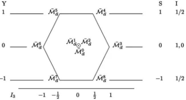
In this way, for fixed ␣ជ=共␣ᐉ,␣u兲, we decompose the basis into the direct sum of irreducible representations of SU共3兲f: a one-dimensional flavor singlet 共denoted byM¯ 0_␣ជ withC2= 0兲 and an eight-dimensional octet共兵M¯ _␣k_ជ其

k=1 8

withC₂= 3兲and the labeling distinguishes between them. These states with their quantum numbers are displayed in Fig.1 where for simplicity we have labeled them byM¯ _␣k_{ជ 共k}

= 0 , 1 , . . . , 8兲. We list兵M¯ _␣k_ជ其

as follows:

M¯ _␣0_ជ

=1₃共␺¯a,␣ᐉ,u␺a,␣_u,u+␺

¯

a,␣ᐉ,d␺a,␣_u,d+␺

¯

a,␣ᐉ,s␺a,␣_u,s兲,

M¯ _␣1_ជ=₃1冑₂共¯␺a,␣ᐉ,u␺a,␣u,u+␺

¯

a,␣ᐉ,d␺a,␣u,d− 2␺

¯

a,␣ᐉ,s␺a,␣u,s兲,

M¯ _␣2_ជ=冑1₆共¯␺a,␣ᐉ,u␺a,␣u,u−␺

¯

a,␣ᐉ,d␺a,␣u,d兲,

M¯ _␣3_ជ

=冑1₃␺¯a,␣ᐉ,u␺a,␣_u,d,

M¯ _␣4_ជ=冑1₃␺¯a,␣ᐉ,u␺a,␣u,s, 共36兲

M¯ _␣5_ជ=冑1₃¯␺a,␣ᐉ,d␺a,␣u,s, M¯ _␣6_ជ

=冑1₃␺¯a,␣ᐉ,d␺a,␣_u,u,

M¯ _␣7_ជ=冑1₃¯␺a,␣ᐉ,s␺a,␣u,u, M¯ _␣8_ជ=冑1₃¯␺a,␣ᐉ,s␺a,␣u,d. The set兵M¯ _␣k_ជ其

is related to兵M¯ ␣ជfជ其by a real orthogonal transformation B. Explicitly, by using the M¯ ␣ជfជ ordering ជf=共u,u兲, 共d,d兲, 共s,s兲, 共u,d兲, 共u,s兲, 共d,s兲, 共d,u兲, 共s,u兲, 共s,d兲 with fixed ␣ជ, B is given by

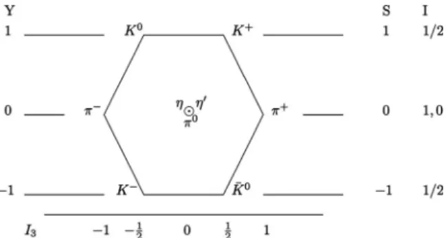
FIG. 1. Graphical representation of the tensor product decomposition 3丢¯3= 8丣1. M¯

␣ជ 0

is the singlet state and the remaining fields兵M¯␣ជ

k_其 k=1 8