Resumo
O objetivo do estudo é avaliar o impacto da restri-ção ao crédito rural sobre a produtividade da terra e a produtividade do trabalho para os agricultores familiares do Brasil. Para estimar esse impacto, foram utilizados dados do Censo Agropecuário de 2006 por município. Para diferenciar os agri-cultores familiares, foram utilizados quartis do índice de mercantilização. O impacto da restrição ao crédito sobre a produtividade da terra e a pro-dutividade do trabalho foi calculado a partir da comparação entre o grupo que recebeu crédito e o que não recebeu crédito, obtido através do escore de propensão (propensity score matching). As es-timativas do efeito médio de tratamento sobre os tratados, quando apresentaram resultados esta-tisticamente signifi cativos, mostraram que o crédi-to aumenta a produtividade do trabalho e da terra e que os valores diferem entre os diferentes níveis de mercantilização dos agricultores familiares e, portanto, requerem políticas distintas.
Palavras-chave
agricultura familiar; mercantilização; crédito ru-ral; propensity score matching.
Códigos JELR15. Marcos de Oliveira Garcias
Universidade Federal da Integração Latino-Americana Ana Lucia Kassouf
Universidade de São Paulo
Abstract
The objective of this study was to evaluate the impact of rural credit on land and labor productivity for Brazilian family farmers and assess factors infl uencing the rural credit approval process. The study employs data contained in the 2006 Brazilian Municipality Agricultural Census and a “trade index” (TI) specifi cally constructed to differentiate family farmers. The impact of credit on land and labor productivity was calculated by comparing the productivity of a group of family farmers that received credit with the productivity of a group of family farmers that were credit restricted. The groups were constructed with the aid of propensity score matching. When statistically signifi cant, the average effect of credit was found to increase the recipient’s productivity of land and labor. It was also found that productivity increases due to the use of credit aligned with the level of the family farmer’s integration into the commercial market and, therefore, one credit policy does not fi t for all Brazilian family farmers.
Keywords
family farming; trade index; rural credit; propensity score matching.
JEL CodesR15.
1
Introduction
On July 24, 2006, the Brazilian National Policy of Family Agriculture and Rural Family Enterprises was enacted by the passage of Law 11.326, also known as the “Law of Family Farming.” Among other things, this document set forth a legal defi nition of “family farming” and established concepts, principles and tools for the formulation of public policies directed towards family farming. This law defi ned a family farmer as an agricultural product producer who meets the following requirements: (i) does not have an area greater than four fi scal modules; (ii) uses primarily family labor; (iii) family income comes principally from economic activities related to the property itself; and (iv) the family manages its property. With this law’s institution, the universe of Brazilian family agriculture was defi ned by a specifi c legal framework that made possible the formulation of a directed public policy.
The 2006 Brazilian Agricultural Census, compiled by the Brazilian In-stitute of Geography and Statistics (IBGE, 2009), identifi ed more than four million family farming units, which represented 84% of Brazil’s farming enterprises. Family farming was found to be a signifi cant participant in the production of plant and animal products, especially those from cassava, beans, corn, coffee, pork and poultry.
The legal defi nition of family farms does not make a distinction between different economic levels of family farming activities, which can range from subsidence farming to farming for economic gain and, possibly, the control of a signifi cant share of a specifi c market. In this sense, Carneiro et al. (2003) address the multifunctionality of family farming, focusing on dif-ferent groups and emphasizing the important role of family farmers as a so-cial group. Conterato (2004) and Perondi (2007) made efforts to identify the social and economic effects of the market entrance by the family farmer.
The 2006 Brazilian Agricultural Census provided data on the per-farm value of production and the per-farm value of quantity sold. It was the fi rst Brazilian census to include these data. In the present study, those data were used to create a new variable: the Trade Index (TI). The TI is a ratio defi ned by the value of the quantity sold divided by the value of the quan-tity produced.1 This variable can be used as an indicator of farmer
integra-tion into the commercial market.
The Brazilian government has used rural credit manipulation as one of its main agricultural policies for some time; however, despite credit’s importance in the process of agricultural modernization, early efforts to employ this tactic have benefi ted mainly large producers (Araujo, 2011; Bacha; Danelon; Belson, 2006). In the mid-1990s, the National Program to Strengthen the Family Farm (PRONAF) was created in an attempt to pro-vide credit to small farming operations. One of this Program’s efforts was designed to reduce impediments generated between the 1960s and 1980s restricting the family farmer’s access to credit.
PRONAF improved access to credit for the family farm, but competition between family farms and non-family farms still hindered the development of many family farm units. More recently, new lines of credit have emerged to extend credit access to more family farms. These efforts include the Na-tional Program of Support to the Middle Rural Producer (PRONAMP2),
which promotes the development of medium-sized rural producers. This study’s analysis of the impact of credit and credit restriction on the productive capacity of family farms did not treat these enterprises as a homogeneous unit but differentiated the farms by their trade index (TI) levels, their location in each of the Brazilian regions, and, of course, their access to credit. Family farmers are considered affected by a credit restric-tion if their demand for credit is not met. The TI level indicates the porrestric-tion of each farm’s production that is sold. Specifi cally, we intend to determine whether access to funds through the use of credit impacts family farm land and labor productivity and evaluate the effect of several specifi c factors on the credit qualifi cation process.
Mattei (2014) evaluated the distribution of PRONAF subsidized rural credit between 2000 and 2010 and discussed aggregate credit distribution in the household sector. The study’s main conclusion is that the use of PRONAF assistance to secure fi nancing is concentrated in the southern Brazilian states and that this credit is focused on the household sector to the exclusion of other sectors, particularly family farmers that were given their land as part of an agrarian reform measure.
Assunção and Alves (2007) gave empirical evidence showing that access to credit is restricted in rural Brazil, after an analysis of the farms in the
country’s fi ve geographical regions. The highest level of credit restriction was found to be in the Northeast.
Resende and Silveira Neto (2009) conducted an evaluation of the effec-tiveness of government subsidized credit in Brazil. The authors concluded that the allocated resources are best employed in the Northeast region and poorly employed in the North and Midwest. This work made it evident that regional factors infl uence credit effectiveness.
Magalhães Neto and Dias et al. (2006) found that PRONAF benefi ciaries in the state of Pernambuco were less effective than producers who did not have access to the program. Magalhães and Filizzola (2005) conducted a study in Paraná that determined that PRONAF had no effect on land productivity; however, the value of output per capita was positive for producer categories B and C, indicating that PRONAF credit policy was effective for some producers.
Kageyama (2003), after analyzing data from nearly 2000 farmer house-holds in 21 municipalities of eight states, found that the presence of PRO-NAF promotes increases in labor and land productivity.
Santos (2010) showed that PRONAF assistance provided an increase of land and labor productivity in Brazil’s Northeast in 2006. However, this analysis involved family farms in aggregate form and did not distinguish between different farms’ levels of trade.
Buainain (2006) and others have determined that family farming is het-erogeneous. It remains to be seen whether results obtained from previous studies are equally valid when family farming is disaggregated into differ-ent groupings, as in the presdiffer-ent study.
2
Methodology
An evaluation of public policy normally seeks to determine the policy’s impact and if there is a causal relationship between that policy and vari-ables of interest. This study estimates the impact of the family farm credit policy on the productivity of family farmer land and labor using observa-tional data and propensity scores.
The initial estimates of the impact of the credit policy were made using multiple regression; thus, it follows that:
0 1
i i i i
Yi , for example, is the productivity of land and labor in agricultural estab-lishmenti; Di is a dummy variable indicating amount of participation in a
rural credit program; Xi the set of covariates; β0 and β1 are the parameters;
ui is the term of the random error and e γ measures the estimated value of
the impact of “treatment” on establishmenti.
According to Angrist & Pischke (2008), the conditional expectation of equation (1) in situations Di = 1 (treated) e Di = 0 (control), is evaluated by
the expressions:
For someXi ,
In this expression, γ is the effect of treatment and , the selection bias. The selection bias corresponds to the correlation between ui and Di , whereas:
The is the counterfactual: what would have happened to the average productivity of land and labor for establishments in the control group if they had been credit beneficiaries; and symbolizes actual average control group productiveness given that the establishments have had their access to credit restricted. If Di
were randomly defined, regression of Yi in function of Di would
es-timate the causal effect of interest γ. To obtain a good estimate of γ , the variable of interest Di must be independent of potential results Yi .
This assumption ensures the hypothesis of conditional independence and allows the causal interpretation of estimated parameters. Under this condition, the treatment and control groups being compared are in fact comparable.
According to Angrist and Pischke (2008, p.11), the observed differ-ence is composed of a causal effect of treatment and a selection bias:
i| i 1
0
i| i 1
E Y D E u D
i | i 0
0
i| i 0
E Y D E u D
i | i 1
i | i 0
i| i 1
i| i 0
E Y D E Y D E u D E u D
i| i 1
i| i 0
0i| i 1
0i| i 0
E u D E u D E Y D E Y D
0i| i 1
E Y D
0i| i 0
E Y D
(2)
(3)
(4)
i| i 1
E u D
i| i 0
E u D
The term measures the average causal effect of rural credit policy on agricultural establishments’ land and labor productivity.
Angrist and Pischke (2008) claim that it is possible to eliminate selec-tion bias if sample establishments with identical observable characteris-tics are selected, the only difference among them being whether they are treated or not. However, given the model’s data sources, the task of select-ing establishments with identical observable characteristics is extremely diffi cult. The control group must be extremely large and the data sources extremely detailed if an individual with the same characteristics is to be found in the treatment group. Rosenbaum and Rubin (1983) proposed pro-pensity score matching (PSM) to solve the common support issues.
In this method, the treatment group will be based on the probability p(X
i ) that the agricultural establishments are credit benefi ciaries from the
covariates vector. The treatment group will be composed of agricultural establishments with characteristics similar to those of the control group except that treatment group establishments are considered credit benefi -ciaries and the control group’s are not.
According to Rosenbaum e Rubin (1983), the propensity score can be used to compare two individuals and is based on .
Following Becker and Ichino (2002), the Average Treatment Effect (ATE) can be written as follows:
Where Y1i is the measure of a treatment group member’s land and labor productivity, and Y0i is the measure of a control group member’s land and
labor productivity.
The fi rst step in calculating the effect of credit is to estimate the pro-pensity score. This can be done using a probability model. The dependent
i| i 1
i| i 0
1i |0i i 1
0i| i 1
E Y D E Y D E Y Y D E Y D
0
E Y Di| i 0
(6)
1i |0i i 1
E Y Y D
Pr
1|
P Xi D X
|
E D X
1 i 0 i | i 1
E Y Y D
1 i 0 i | i 1,
E E Y Y D p
Xi
1 i | i 1,
0 i | i 0,
| i 1E E Y D p E Y D p D
variable is a dummy indicating whether the family farms were considered participants or non-participants in the rural credit program. For the logit model, it is:
The probability of one matched establishment receiving treatment will be defi ned by equation 9 below:
After the propensity score is estimated, following assumption , the distribution of covariates among treatment and control groups should be similar. The propensity score were submitted to at-test to determine whether the average of the differences between groups was not statistically different from zero after matching.
The calculated p(X
i ) for the effect of credit τ | Di = 1 will be:
The evaluation of the government’ rural credit policy in Brazil presented in this study is intended to answer the following questions: Do Brazil’s rural credit policies impact its benefi ciaries’ land and labor productivity indicators? What are these impacts? How can one say that any impacts
are a result of the policies, when impacts noticeably differ among its intended benefi ciaries?
In equation (1), Yi is the variable of interest (land and labor productivity
i ) and Di is a dummy variable that indicates either treatment or control group member, with Di = 1 representing a member of the treatment group,
and Di = 0 representing a member of the control group; Y1i is a measure
of a treatment group member’s land and labor productivity, and variable Y0i is a measure of a control group member’s land and labor productivity.
Different methodologies can be used to propensity score match, i.e., selecting members belonging to the treatment and control groups, each of which adopts a specifi c weighting. However, we used the nearest neigh-bor without replacement, nearest neighneigh-bor with replacement and the ker-(8)
' 1
Pr 1|
1 i
i i
D X
e
X
Pr
i 1|
( i| )p Xi D Xi E D Xi (9)
|
i i
X D p Xi
(10)
1 1,
| | | 1
i i i i
D Ep X D p X Di
nel methods in this work. These three methods were employed to check the results’ robustness.
In the matching method that considered the nearest neighbor without replacement, a member in the control group with the closest score to the individual considered in the treatment group is selected, after that the indi-vidual in the control group is removed from the sample. Using the replace-ment method, the fi ve nearest neighboring municipalities with the most similar covariate scores are compared and replaced from the sample. Using the kernel method, an individual in the control group with a score most similar to a member of the treatment group is selected.
3
Data source
Data used in this study came from the “Family Farming: First Results” sec-tion of the 2006 Brazilian Agricultural Census. This new statistical refer-ence was made possible by the establishment of criteria legally defi ning a “family farm” (Law 11.326), and was compiled by the Brazilian Ministry of Agricultural Development in cooperation with IBGE.
The publication of “First Results” was not the fi rst attempt to measure family farming activities but followed a study conducted through a part-nership between the Food and Agriculture Organization and the Brazil-ian National Institution of Agricultural Reform (FAO/INCRA), which used statistics from the 1995-96 Census; however, information available from that census were not designed for this purpose.
The concept of family farm agriculture is related to the family unit while the property is related to the production unit. Although the most common situation is a family linked to only one establishment, there are cases of families that farm more than one agricultural establishment. In the current study there may be a slight overestimation of the population involved in family farming as one family unit is assumed to have done the work at each family farm.
3.1 Empirical strategy
In this study, the unit of interest is the agricultural establishment and wheth-er or not that establishment received some sort of rural credit. It would have been helpful if the IBGE site3 provided 2006 microdata that broke down the
municipal data into individual farms, but due to confi dentiality issues, the site provides only information aggregated by municipality4. The Census
mi-crodata can be accessed, but access is both too diffi cult and too costly for our endeavor.5 We were therefore forced to address the same objectives using
the municipality rather than the individual family farm as the research unit. The 2006 Agricultural Census presents the following information by municipality: number of agricultural establishments that did not receive funding, number of family farms that were not approved to receive fund-ing, number of non-family agricultural establishments that were not ap-proved to receive a funding, number of family agricultural establishments that obtained funding, number of non-family agricultural establishments that obtained funding, and the total value of family farm funding.
Table 1 Proportion of establishments by the reasons why they did not obtain funding in Brazil and by regions
Type of failed to obtain fi nancing
Brazil and regions
Did not obtain
No war-ranty
Do not know how to obtain
Bureau-cracy
Absence of previ-ous pay-ment
Afraid of debt
Others Do not apply
Brazil 84.25 1.62 1.32 7.08 2.75 18.42 10.87 42.21
North 86.86 2.55 3.44 12.32 2.72 14.79 11.89 39.15
Northeast 88.89 1.94 1.44 7.3 3.82 23.86 14.6 35.94
Southeast 76.36 0.67 0.7 4.81 1.39 14.76 5.37 48.66
South 83.22 1.12 0.48 4.93 1.1 10.63 5.44 59.53
Midwest 69.03 1.55 0.76 8.55 2.15 10.45 8.68 36.89
Source: Authors’ estimation based on 2006 Brazilian Agricultural Census.
3 http://sidra.ibge.gov.br/
4 A “municipality” in Brazil would be considered a county in many other counties, as it contains both urban and rural areas. In this paper the term “municipality” will continue to be employed, but it can be considered to represent a county.
Table 1 shows the proportion of establishments in Brazil by the rea-sons why they did not obtain funding, by region and by municipality in accordance with the 2006 Agricultural Census. It can be observed that 42.21% of family farming establishments (84.25% of total) did not apply for credit. Of the total family farming establishments in a mu-nicipality, the portion that did not demand credit was removed from our sample.
Those eligible family farmers that applied for some credit but were denied are considered to have had their credit restricted. According to Chaves et al. (2001, p.55-56), the credit restriction concept is relative, arising from the comparison between demand for credit funds and the available supply. A family farmer that does not demand credit cannot be considered restricted while those who are eligible for but are de-nied credit have a credit restriction. Starting from this defi nition, it was possible to create a credit restriction variable to differentiate establish-ments that effectively suffered restriction from those that were rela-tively free from restriction. This dummy variable is either 0 or 1: One, if the majority of the municipal establishments suffered restriction; 0 if the minority of the municipal establishments suffered restriction. The variable will be used in the land and labor productivity comparison to distinguish between family farms that received credit and those that suffered a credit restriction.
Table 2 presents the descriptive statistics of the credit restriction variable. The regions with the highest share of the total data are the Northeast, Southeast and South, with 1,765, 1,515 and 1,169 munici-palities, respectively.
Table 2 Descriptive statistics of credit restriction variable
Brazil and regions
Number of observations
Mean S.D. Min Max
Brazil 5312 0.640 0.246 0 1
Midwest 431 0.698 0.194 0.000 1
Northeast 1765 0.776 0.127 0.024 1
North 432 0.825 0.131 0.167 1
Southeast 1515 0.635 0.218 0.000 1
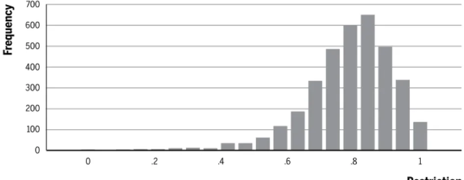
South 1169 0.355 0.213 0.000 1
Figure 1 Dispersion of restriction values among the municipalities of Brazil
Source: Authors’ estimation based on 2006 Brazilian Agricultural Census.
Figure 2 Dispersion of restriction values among the municipalities of Midwest region
Source: Authors’ estimation based on 2006 Brazilian Agricultural Census.
Figure 3 Dispersion of restriction values among the municipalities of Northeast region
Source: Authors’ estimation based on 2006 Brazilian Agricultural Census. 0
75
50
25 150
125
100
0 .2 .4 .6 .8
Fr
equency
1
Restriction
0 400
300
200
100 600
500 700
0 .2 .4 .6 .8
Fr
equency
1
Restriction
0 40
30
20
10 80
70
60
50
.2 .4 .6 .8
Fr
equency
1
Figure 4 Dispersion of restriction values among the municipalities of North region
Source: Authors’ estimation based on 2006 Brazilian Agricultural Census.
Figure 5 Dispersion of restriction values among the municipalities of Southeast region
Source: Authors’ estimation based on 2006 Brazilian Agricultural Census.
Figure 6 Dispersion of restriction values among the municipalities of South region
Source: Authors’ estimation based on 2006 Brazilian Agricultural Census. 0
300
200
100 600
500 700
400
0 .2 .4 .6 .8
Fr
equency
1
Restriction
0 30
20
10 60
50
40
0 .2 .4 .6 .8
Fr
equency
1
Restriction
0 75
50
25 150
125
100
0 .2 .4 .6 .8
Fr
equency
1
In terms of credit restriction averages, there is great heterogeneity among the fi ve regions. Midwest and Southeast are closest to the national average, with 69% and 63% of the establishments that demanded credit affected by credit restriction. North and Northeast regions have the highest restriction averages, with 82% and 77% of farms that demanded credit rejected. In contrast, the Southern region has a credit restriction average of only 35%.
Figures 1 to 6 show the dispersion of restriction values within Brazil. As the family farm population affected by credit restriction differs from region to region, the regional restriction values rather than the average na-tional value were used in the creation of the control and treatment groups.
This study employed the following model to estimate the propensity score in each of the geographic regions:
Di* is a dummy variable, the value of which denotes whether the majority or minority of municipal establishments receive credit. The explanatory variables represent characteristics of producers and production, β s are the parameter of the model and ui is the random error term. Each trade index group will have a specifi c estimation.
The variables are defi ned below:
Di* - dummy variable; municipalities in which more than half of the demanding establishments received credit take a value of 1 (treated); municipalities in which less than half received credit take a value of 0 (control);6;
v_aduboi - Percentage of municipal establishments that use some type of fertilizer;
v_condicaoi - Percentage of establishments with manager/owner;
6 Tests were conducted with different specifi cations as to the treatment group and control group (40% -40% 45% -45% 35% -35%), however, the most robust results were found by separating municipalities that present restricting credit and those that exhibit 50%.
*
0 1 _ 2 _ 3 _
i i i i
D v adubo v condicao v cpragasdoenca
12v invest_ i 13v divida_ i ui
4v coopclasse_ i 5v experien_ i 6v internet_ i 7v idade_ i
8v escolaridade_ i 9v orient_ i 10v prepsolo_ i 11v masculino_ i
v_cpragasdoencai - Percentage of establishments that take measures to control pests and diseases;
v_coopclassei - Percentage of establishments associated with coop-eratives and/or professional associations;
v_experieni - Percentage of establishments that have a manager with 10 years or more of experience;
v_interneti - Percentage of establishments with internet access;
v_idadei - Percentage of establishments where the manager is at
least 35 years old;
v_escolaridadei - Percentage of establishments in which the man-ager has a least high school degree;
v_orienti - Percentage of establishments that receive technical,
pub-lic or private advice;
v_prepsoloi - Percentage of establishments that perform some type of soil tillage;
v_masculinoi - Percentage of establishments in which the manager
is male;
v_investi - Percentage of establishments that make some type of investments;
v_dividai - Percentage of establishments that have existing debts;
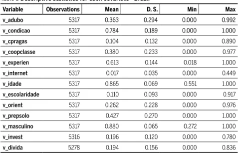
Table 3 shows the mean, standard deviation, minimum, maximum and the number of observations for each variable. The v_invest and v_divida variables have fewer observations due to IBGE’s confi dentiality rules. According to IBGE criterion, if a municipality has 1-3 establishments with information for a particular characteristic, that information will not be divulged.
Variables v_condicao, v_experien, v_idade and v_masculino have mean val-ues above 60%, which indicates that most family farmers in the munici-palities’ sample are owners of the property they farm, that most managers have over 10 years’ experience, that most managers are at least 35 years old and, as might be expected, that most managers are male, respectively.
The following are the land and labor productive variables’ defi nitions: (i) Gross land productivity - the total value of production divided by the total area of the family farming establishment;
(ii) Gross labor productivity - the total value of production divided by the number of workers employed in production.
restric-tion on enterprises from different TI levels was assessed. The control and treatment groups’ populations were separated into four different catego-ries determined by TI value, making it possible to identify differences in treatment and productivity associated with the enterprises’ TI level.
The TI quartiles were defi ned as follows:
1st quartile – family farms that sold 0% to 25% of their production;
2nd quartile - family farms that sold 25% to 50% of their production;
3rd quartile - family farms that sold 50% to 75% of their production;
4th quartile - family farms that sold 75% to 100% of their production.
Table 3 Descriptive statistics for each covariate - Brazil
Variable Observations Mean D. S. Min Max
v_adubo 5317 0.363 0.294 0.000 0.992
v_condicao 5317 0.784 0.189 0.000 1.000
v_cpragas 5317 0.104 0.132 0.000 0.890
v_coopclasse 5317 0.380 0.233 0.000 0.977
v_experien 5317 0.613 0.144 0.018 1.000
v_internet 5317 0.017 0.035 0.000 0.449
v_idade 5317 0.865 0.069 0.551 1.000
v_escolaridade 5317 0.110 0.093 0.000 0.917
v_orient 5317 0.262 0.228 0.000 0.976
v_prepsolo 5317 0.427 0.270 0.000 1.000
v_masculino 5317 0.880 0.065 0.272 1.000
v_invest 5316 0.196 0.120 0.000 0.780
v_divida 5278 0.194 0.156 0.000 0.836
Source: Authors’ estimation based on 2006 Brazilian Agricultural Census.
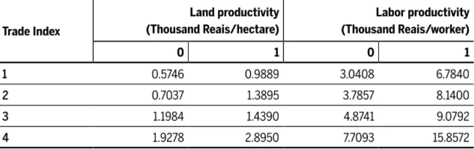
Table 4 shows average productivity of land and labor for each quartile of both the control (0) and the treatment groups (1). The distribution was divided into four sections according to the trade index variable to create smaller but more homogeneous family farm groups.
more than half of the stablishments in the municipalities have access to credit – and the levels of productivity.
Table 4 Average productivity of land and labor for each quartile of both the control (0) and the treatment groups (1) - Brazil
Trade Index
Land productivity (Thousand Reais/hectare)
Labor productivity (Thousand Reais/worker)
0 1 0 1
1 0.5746 0.9889 3.0408 6.7840
2 0.7037 1.3895 3.7857 8.1400
3 1.1984 1.4390 4.8741 9.0792
4 1.9278 2.8950 7.7093 15.8572
Source: Authors’ estimation based on 2006 Brazilian Agricultural Census.
4
Results
This section presents the results of the study of the effect of credit on the productivity of land and labor and the effect of producer characteristics on the credit restriction process.
4.1 Probability of establishments in municipalities suffering credit
restriction
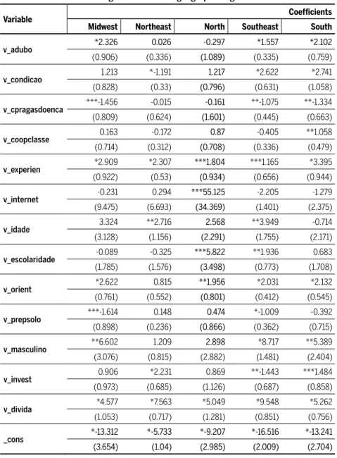
Results from the logit model make it possible to discuss the effect of each covariate on the probability of credit restriction in each geographic region (see: Table 5). Not all the variables’ coeffi cients were statistically signifi -cant at a 10% level in their ability to explain the probability of establish-ments in a municipality suffering credit restriction.
Some producer characteristics were found to greatly infl uence the credit restriction process. Results showed that in all regions, the higher the per-centage of establishments in a municipality in which the producer has over 10 years of experience, the lower the probability of credit restriction. The magnitude of this effect is even greater in the South, the region that receives the largest share of rural credit resources.
in a municipality, the lower the probability of credit restriction, which may be directly related to the need for credit to provide working capital. This result was signifi cant and positive in all geographical regions.
Table 5 Coeffi cients of the logit model in each geographic region
Variable Coeffi cients
Midwest Northeast North Southeast South
v_adubo *2.326 0.026 -0.297 *1.557 *2.102 (0.906) (0.336) (1.089) (0.335) (0.759)
v_condicao 1.213 *-1.191 1.217 *2.622 *2.741 (0.828) (0.33) (0.796) (0.631) (1.058)
v_cpragasdoenca ***-1.456 -0.015 -0.161 **-1.075 **-1.334 (0.809) (0.624) (1.601) (0.445) (0.663)
v_coopclasse 0.163 -0.172 0.87 -0.405 **1.058 (0.714) (0.312) (0.708) (0.336) (0.479)
v_experien *2.909 *2.307 ***1.804 ***1.165 *3.395 (0.922) (0.53) (0.934) (0.656) (0.944)
v_internet -0.231 0.294 ***55.125 -2.205 -1.279 (9.475) (6.693) (34.369) (1.401) (2.375)
v_idade 3.324 **2.716 2.568 **3.949 -0.714 (3.128) (1.156) (2.291) (1.755) (2.171)
v_escolaridade -0.089 -0.325 ***5.822 **1.936 0.683 (1.785) (1.576) (3.498) (0.773) (1.708)
v_orient *2.622 0.815 **1.956 *2.031 *2.132 (0.761) (0.552) (0.801) (0.412) (0.545)
v_prepsolo ***-1.614 0.148 0.474 *-1.009 -0.392 (0.898) (0.236) (0.866) (0.362) (0.715)
v_masculino **6.602 1.209 2.898 *8.717 **5.389 (3.076) (0.815) (2.882) (1.481) (2.404)
v_invest 0.906 *2.231 0.869 **-1.443 ***1.484 (0.973) (0.685) (1.126) (0.687) (0.858)
v_divida *4.577 *7.563 *5.049 *9.548 *5.262 (1.053) (0.717) (1.281) (0.851) (0.756)
_cons *-13.312 *-5.733 *-9.207 *-16.516 *-13.241
(3.654) (1.04) (2.985) (2.009) (2.704)
Source: Authors’ estimation based on 2006 Brazilian Agricultural Census (s.d).
Results also showed that the higher the percentage of establishments in a municipality that receive technical guidance, the lower the probability of credit restriction. This result was observed in all regions except the North-east. It seems that technical assistance, for the most part conducted by technicians from state agencies, facilitates credit approval.
Other variables, such as use of fertilizers, land ownership, the farm manager’s gender, and internet access, also showed signifi cant results in some regions.
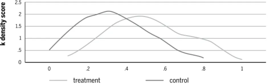
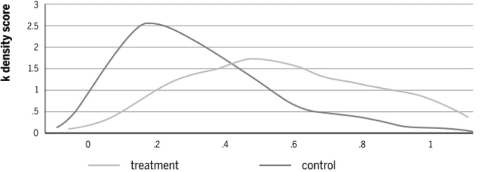
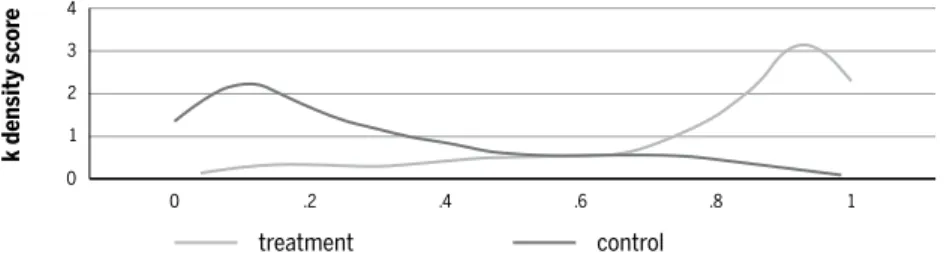
Scores generated by the logit model also serve as indicators of the cor-relation between the treatment and control groups, which is useful when selecting municipalities in each group for comparison. Figures 7 to 11 graphically illustrate the treatment and control group’s density function scores for all geographic regions. The curve in bold represents the estimat-ed scores for control group municipalities, and the fi ner curve represents scores for treatment group municipalities.
One can observe that in all regions there is ashared area below the treat-ment and control groups’ density curves. Similar and therefore comparable municipalities are included in this region, i.e., they will have similar co-variate scores, differing only in restriction or access to credit. Municipali-ties from the treated and control groups occupying this shared area were then selected for matching and their land and labor productivity values were compared. Note that the major criticism of this method of selection is its inability to control and account for unobservable effects, which can lead to bias and inconsistency in parameter estimates.
Figure 7 Function of density of scores generated by the logit model by treatment and control groups of Midwest region
Source: Authors’ estimation based on 2006 Brazilian Agricultural Census. 0
1.5
1
.5 2 2.5
0 .2 .4 .6 .8
k density
scor
e
1
Figure 8 Function of density of scores generated by the logit model by treatment and control groups of Northeast region
Source: Authors’ estimation based on 2006 Brazilian Agricultural Census.
Figure 9 Function of density of scores generated by the logit model by treatment and control groups of North regionn
Source: Authors’ estimation based on 2006 Brazilian Agricultural Census.
Figure 10 Function of density of scores generated by the logit model by treatment and control groups of Southeast region
Source: Authors’ estimation based on 2006 Brazilian Agricultural Census. 0
1.5
1
.5 2 2.5 3
0 .2 .4 .6 .8
k density
scor
e
1
treatment control
0 1.5
1
.5 2 2.5
0 .2 .4 .6 .8
k density
scor
e
1
treatment control
0 1.5
1
.5 2 2.5
0 .2 .4 .6 .8
k density
scor
e
1
Figure 11 Function of density of scores generated by the logit model by treatment and control groups of South region
Source: Authors’ estimation based on 2006 Brazilian Agricultural Census.
As noted in the Methodology section, the matching was performed using the nearest neighbor without replacement, replacement with the fi ve clos-est neighbors, and the Kernel methods. Municipalities were matched for the four different TI levels and for all geographical regions.
An average difference test for each of similar municipalities’ covariates was conducted to verify whether the matching was carried out satisfacto-rily. It was determined that the null hypothesis where means are the same should not be rejected, indicating that there is no difference between the average of the respective covariates for the treatment and control group municipalities. The results were not signifi cant for almost all covariates, showing that the treatment and control groups are homogeneous.7
The next section shows the Average Treatment Effect (ATE) on land and labor productivity by region.
4.2 The effect of credit restriction on land productivity
Productivity differences between similar control and treated municipali-ties were used to determine the ATE in the fi ve regions and at the four TI levels. Table 6 indicates the calculated average effect of no credit restric-tion on land productivity.
The fi rst point worth highlighting is that there is a substantial difference in land productivity between treatment and control groups when compar-ing regions and different TI levels; however, not all results were statistical-ly signifi cant. This indicates that when comparing similar municipalities,
7 To check the results of tests of averages for each of the covariates see Garcias 2014.
0 3
2
1 4
0 .2 .4 .6 .8
k density
scor
e
1
there is often no land production difference that can be correlated with credit restriction, but that credit access and restriction have different ef-fects depending on the farmer’s TI value and production region.
Table 6 Average effect of treatment on land productivity in different quartiles of the trade index, by regions in Brazil
Land productivity (thousands reais/hectare)
Region TI Nearest neighbour without replacement
Kernel 5 nearest neighbour with replacement
ATE S.D. t-test ATE S.D. t-test ATE S.D. t-test
Midwest
1 -0.149 0.148 -1 -0.035 0.18 -0.19 -0.065 0.111 -0.58
2 -0.012 0.121 -0.1 0.106 0.063 ***1.680 -0.259 0.127 **-2.040
3 -0.074 0.138 -0.54 -0.009 0.089 -0.1 -0.226 0.198 -1.14
4 0.24 0.146 ***1.640 0.283 0.139 **2.040 0.15 0.163 0.92
North-east
1 0.005 0.083 0.05 0.101 0.083 1.22 0.084 0.082 1.02
2 -0.24 0.281 -0.85 0.169 0.132 1.28 0.178 0.467 0.38
3 0.259 0.488 0.53 0.176 0.596 0.3 0.15 0.505 0.3
4 0.908 0.982 0.92 1.185 0.988 1.2 0.894 0.976 0.92
North
1 -0.0195 0.0318 -0.61 -0.035 0.0536 -0.66 -0.008 0.034 -0.26
2 -0.0296 0.098 -0.3 -0.006 0.1129 -0.06 -0.026 0.108 -0.25
3 -0.159 0.117 -1.35 -0.226 0.2059 -1.1 -0.187 0.159 -1.18
4 -0.046 0.112 -0.41 -0.017 0.1782 -0.1 -0.009 0.13 -0.07
South-east
1 0.282 0.101 *2.78 0.282 0.142 *1.99 0.222 0.37 0.6
2 0.287 0.245 1.17 0.181 0.268 0.68 0.278 0.314 0.88
3 -0.185 0.182 -1.02 -0.132 0.23 -0.58 -0.13 0.208 -0.63
4 -0.057 0.779 -0.07 0.883 0.812 1.09 0.963 0.915 1.05
South
1 0.31 0.29 1.07 -0.376 0.823 -0.46 -0.12 0.664 -0.18
2 0.213 0.19 1.12 -1.29 0.605 *-2.13 -1.155 0.364 *-3.17
3 0.348 0.143 *2.43 0.296 0.332 0.89 0.198 0.315 0.63
4 3.367 3.416 0.99 3.367 3.421 0.98 3.085 3.423 0.9
Source: Authors’ estimation based on 2006 Brazilian Agricultural Census.
Note: ***, **, * signifi cant at 1% level, 5% and 10% level respectively.
produc-tion). In contrast, results for the group of municipalities in the same region but in the 2nd TI quartile become negative and signifi cant when analyzed using either the kernel or without replacement models
These results indicate that rural credit policy often does have a positive effect on land productivity, but that effect depends on the family farmer’s region and TI value; e.g., Midwest (2nd and 4th TI quartiles), Southeast (1st and 4th TI quartiles) and South (3rd and 4th TI quartiles).
These estimates confi rm results from studies by Anjos et al. (2004) and Silva (2008). Those authors found that access to credit has a positive ef-fect on local development, but only in specifi c locations. There is still an indication that credit access can have a negative effect in relation to land productivity, as the results for most regions’ establishments in the 2nd TI quartile demonstrate. Santos (2010), evaluating aggregated family farmers, noted that there was an increase in land productivity for establishments that suffered restricted credit only in the Northeast region.
4.3 The effect of credit access and restriction on labor productivity
Table 7 shows the calculated average effect of credit on labor productivity. As with the land productivity results, there is a gap between the treatment and control group results and substantial differences among regions and TI levels; again highlighting that the effect of credit on family farmers is not ho-mogeneous. Although many of results for labor productivity were not sta-tistically signifi cant, they were more robust than those for land productivity. Labor production values for municipalities in the Midwest, Southeast and South were found to be positively affected by credit. In these regions, labor productivity values were higher for municipalities in which the aver-age family farmer was at a higher TI level and the majority received credit approval than for municipalities also at a higher average TI level but in which the majority of family farmers were credit restricted. The effects var-ied by region, with the labor productivity value differential between these two types of municipalities reaching R$ 3,970/worker in the Midwest.
worker while the value of production for the average family farmer in the group of municipalities ranked in the 4th TI level was R$6,945/worker.
Table 7 Average effect of treatment on labor productivity in different quartiles of the trade index, by regions in Brazil
Land productivity (thousands reais/worker)
Region TI Nearest neighbour without replacement
Kernel 5 nearest neighbour with replacement
ATE S.D. t-test ATE S.D. t-test ATE S.D. t-test
CO
1 -0.29 1.034 -0.28 0.423 0.995 0.43 -0.202 0.849 -0.24
2 -1.856 3.327 -0.56 1.295 0.848 1.53 -9.367 3.48 *-2.690
3 1.669 1.244 1.34 2.179 1.402 1.55 1.173 1.468 0.8
4 3.972 2.247 ***1.770 4.198 2.234 ***1.880 3.368 2.282 1.48
NE
1 0.142 0.312 0.45 0.159 0.272 0.58 0.131 0.388 0.34
2 -0.179 0.492 -0.36 0.385 0.355 1.08 0.25 0.814 0.31
3 0.618 0.793 0.78 0.25 0.993 0.25 0.327 0.821 0.4
4 2.757 3.438 0.8 2.898 3.467 0.84 2.762 3.428 0.81
N
1 -0.367 0.394 -0.93 -0.32 0.525 -0.61 -0.28 0.41 -0.68
2 -0.6 0.796 -0.75 0.3562 0.595 0.6 -0.952 1.084 -0.88
3 0.0072 0.533 0.01 -1.276 0.779 -1.62 -0.396 0.678 -0.58
4 -0.008 0.708 -0.01 -0.18 1.073 -0.17 0.256 0.771 0.33
SE
1 2.528 1.154 *2.19 1.962 1.514 1.3 2.039 1.301 1.57
2 1.807 1.476 1.22 1.946 1.674 1.16 1.585 1.789 0.89
3 0.482 1.158 0.42 1.046 1.557 0.67 -0.191 1.323 -0.14
4 6.945 3.14 *2.21 7.91 3.328 *2.38 7.517 3.708 *2.03
S
1 1.129 1.242 0.91 -2.987 4.194 -0.71 -1.18 3.019 -0.39
2 2.505 0.911 *2.75 -5.897 2.529 *-2.33 -2.533 1.618 -1.57
3 2.969 0.739 *4.02 0.843 1.778 0.47 0.666 1.622 0.41
4 6.884 7.46 0.92 6.674 7.642 0.87 5.274 7.56 0.7
Source: Authors’ estimation based on 2006 Brazilian Agricultural Census.
Note: ***, **, * signifi cant at 1% level, 5% and 10% level respectively.
Kageyama (2003) also found that access to credit promotes increases in labor productivity, but did not examine whether the effect was differenti-ated. The sample in that paper was limited to eight states.
how integrated the family farm is into the commercial market and the farm’s location.
5
Conclusion
This study evaluated the effects of family farm credit policy on the land and labor productivity of farmers located in different regions and at dif-ferent levels of market integration, as determined by the farmer’s Trade Index (TI) value.
The credit restriction process was also examined while conducting the study; however, as family farming was covered in aggregate form, it was not possible to ascribe results to a particular family farm group. Some pro-ducer characteristics were found to be important in determining which eligible family farmer received credit and which did not. Among these de-terminants for credit approval it was found that if the producer had more than 10 years of farming experience the possibility of approval improved. Other variables that increased chances for credit approval were the prior approval for credit and access to technical assistance.
The effect of credit on productivity were differentiated among farms at different TI levels, as was to be expected. When statistically signifi cant, the results were more positive in municipalities where family farm TI av-erages were in the last quartile of the TI distribution, that is, farmers who marketed more than 75% of their agricultural production.
Although some results are not statistically signifi cant, this work showed that credit restriction has a differential effect when family farming is dis-aggregated into specifi c groups according to the degree of market inte-gration. In general, the effect of rural credit policy on the productivity of land and labor were positive; however, it may also have effects on other production or social indicators that were not examined. Credit can also be seen as a mechanism to address the needs of family farmers associated with the group’s multifunctional role.
funds from a government subsidized credit program be made contingent on the acceptance of technical assistance when reasonable, so the family farmer can get advice on proper resource allocation.
Within the scope that defi nes family farming, there are different sub-segments, here differentiated using values from a Trade Index designed for use in this study. The model’s results confi rm that the effects of rural credit restriction depend on whether the family farming community is more or less integrated into the farm product market; thus, it is concluded that dis-similar groups of family farms require different policies.
References
ANGRIST, J.D.; PISCHKE, J. Mostly Harmless Econometrics: an empiricists companion. Princeton: Princeton University Press, 2008. 392 p.
ARAÚJO, P. F. C. Política de crédito rural: refl exões sobre a experiência brasileira. Textos para Discussão CEPAL-IPEA, 37. Brasília: CEPAL/IPEA, 2011. 65 p.
ASSUNÇÃO, J. J.; ALVES, L. S. Restrições de crédito e decisões intra-familares. Revista Brasileira de Economia, Rio de Janeiro, v. 61, n. 2, p. 201-229, 2007.
BACHA, C. J. C.; DANELON, L.; BEL FILHO, E. D. Evolução da taxa de juros real do crédito rural no Brasil, período de 1985 a 2003. Teoria e Evidência Econômica, Passo Fundo, v. 14, n. 26, p. 43-69, 2006.
BECKER, S; ICHINO, A. Estimation of Average Treatment Effects Based on Propensity Scores. The Stata Journal, Nova York, v.2, n.4, p. 358-377, 2002.
BNDE. Banco Nacional do Desenvolvimento Econômico e Social. Programas e Fundos. 2015. Available at < http://www.bndes.gov.br/SiteBNDES/bndes/bndes_pt/Institucional/Apoio _Financeiro/Programas_e_Fundos/pronamp.html>. Accessed on October 01, 2015. BUAIANAIN, A. M. Agricultura familiar, agroecologia e desenvolvimento sustentável: questões para
o debate. Brasília: IICA, 2006. 135 p.
CARNEIRO, M. J.; MALUF; R. (Orgs.). Para além da produção: multifuncionalidade e agricul-tura familiar. Rio de Janeiro: MUAD, 2003. 230 p.
CHAVES, R. A.; SANCHEZ, S.; SCHOR, S.; TESLIUC, E. Ficancial markets, credit constraint, and investiment in rural Romania. Washington: The World Bank, 2001. 136 p.
CONTERATO, M. A. A mercantilização da agricultura familiar do Alto Uruguai/RS: um estudo de caso no município de Três Palmeiras. 2004. 192 p. Dissertação (Mestrado em Desen-volvimento Rural) - Universidade Federal do Rio Grande do Sul. Faculdade de Ciências Econômicas. Programa de Pós-Graduação em Desenvolvimento Rural , Porto Alegre, 2004. GARCIAS, M. O. Agricultura familiar e os impactos da restrição ao crédito rural: uma análise para
Programa de Pós-Graduação em Economia Aplicada, Piracicaba, 2014.
INSTITUTO BRASILEIRO DE GEOGRAFIA E ESTATÍSTICA. Censo Agropecuário 2006. Agri-cultura Familiar. Primeiros resultados. Brasil, Grandes Regiões e Unidades da Federação. MDA/ MPOG, 2009. 267 p.
KAGEYAMA, A. Produtividade e renda na agricultura familiar: efeitos do PRONAF-crédito. Agricultura em São Paulo, São Paulo, v. 50, n.2, p. 1-13, 2003.
MAGALHÃES, A. M.; FILIZZOLA, M. The family farm program in Brazil: the case of Parana. In: CONGRESSO BRASILEIRO DE ECONOMIA, ADMINISTRAÇÃO E SOCIOLOGIA RURAL, 2005, Ribeirão Preto. Anais.... Ribeirão Preto: Editora, 2005. 20 páginas. MAGALHÃES, A. M.; NETO, R. S.; DIAS, F. D. M.; BARROS, A. R. A experiência recente do
PRONAF em Pernambuco: ama análise por meio de propensity score. Economia Aplicada, Ribeirão Preto, v. 10, n.1, p. 57-74, 2006.
MATTEI, L. Evolução do crédito do PRONAF para as categorias de agricultores familiares A e A/C entre 2000 e 2010. Revista Econômica do Nordeste, v. 45, p. 58-69, 2014.
PERONDI, M. A. Diversifi cação dos meios de vida e mercantilização da agricultura familiar. 2007. 245 p. Tese (Doutorado em Desenvolvimento Rural) - Universidade Federal do Rio Grande do Sul. Faculdade de Ciências Econômicas. Programa de Pós-Graduação em De-senvolvimento Rural, Porto Alegre, 2007.
ROSEMBAUM, P. R., RUBIN, D. B. The central role of propensity score in observational stud-ies for causal effects. Biometrika, Nova York, v.70, n.1, p. 41-55, 1983.
SANTOS, R. B. N. dos. Impactos da restrição ao crédito rural nos estabelecimentos agropecuários brasileiros. 2010. 123 p. Tese (Doutorado em Economia Aplicada) – Universidade Federal de Viçosa, Viçosa, 2010.
SILVA, A. M. A.; RESENDE, G. M.; SILVEIRA NETO, R. M. Efi cácia do gasto público: uma avaliação do FNE, FNO e FCO. Estudos Econômicos, v. 39, n. 1, p. 89-125, 2009.
About the authors
Marcos de Oliveira Garcias - [email protected]
Instituto Americano de Economia, Sociedade e Política (ILAESP), Universidade Federal da Integração Latino-Americana (UNILA), Foz do Iguaçu – PR.
Ana Lucia Kassouf - [email protected]
Universidade de São Paulo, Piracicaba – SP.
The authors would like to thank Professor Rodolfo Hoffmann for comments and suggestions on earlier versions of this work. The remaining errors are the sole responsibility of the authors.
About the article