Fabiana Rocha Paulo Picchetti**
Summary: 1. Introduction; 2. Fiscal adjustment in Brazil: an informal assessment; 3. Fiscal adjustment in Brazil: a model of changes in regime; 4. Size and composition of fiscal adjustments; 5. Conclusions.
Keywords: fiscal adjustment; magnitude; composition; Markov chain.
JEL codes: E62; E65.
Two questions are addressed in this paper. The first one is the determination of periods of fiscal consolidation and fiscal stimu-lus. The second one is the importance of the composition of fiscal adjustments for their success, defined as a declining debt to GDP ratio. We, characterize 1994 and 1999 as points of fiscal consol-idation. The 1994 consolidation can not be considered successful since after that period the debt to GDP ratio has grown contin-uously. The adjustment can be characterized as a type 2 adjust-ment (Alesina and Perotti (1997)) in the sense that cuts were made mainly in public investment, while government wages and transfers remained almost unchanged. This type of adjustment usually has a low likelihood of being a success.
Duas quest˜oes s˜ao tratadas neste artigo. A primeira ´e a deter-mina¸c˜ao dos per´ıodos de consolida¸c˜ao fiscal e est´ımulo fiscal. A segunda quest˜ao ´e a importˆancia da composi¸c˜ao dos ajustamen-tos fiscais para o seu sucesso, definido como um decl´ınio na razo d´ıvida/PIB. N´os, caracterizamos 1994 e 1999 como pontos de con-solida¸c˜ao fiscal. A concon-solida¸c˜ao de 1994 n˜ao pode ser considerada um sucesso pois nos anos seguintes a raz˜ao d´ıvida/PIB cresceu con-tinuamente. O ajustamento pode ser considerado como um ajusta-mento do tipo 2 (Alesina and Perotti, 1997) no sentido de que foram feitos cortes principalmente no investimento p´ublico, enquanto os sal´arios e transferˆencias permaneceram praticamente inalterados. Este tipo de ajustamento geralmente tem uma baixa probabilidade de sucesso.
*
This paper was received in feb. 2001 and approved in apr. 2002. We would like to thank Aod Cunha de Nobes Junior, Maria Carolina Leme and two anonymous referees for their valuable comments and suggestions. All remaining errors are our entire responsability.
**
Department of Economics, University of S˜ao Paulo, S˜ao Paulo, Brazil
1.
Introduction
Although the great variation in budget balances and the increasing government debt have been worrying Brazilian economists for quite a while, there are not many empirical analysis of fiscal changes in Brazil. It would be useful , therefore, to have a more accurate analysis of the fiscal performance over the recent period. The purpose of this paper is to try to fill in this gap. Two questions are addressed.
The first one is the determination of periods of fiscal consolidation and fiscal stimulus. Which episodes can be classified as an experience of fiscal consolidation? In order to answer this question we initially follow McDermott and Wescott (1996) and Alesina and Perotti (1997). They classify expansions/consolidations according to an arbitrary criteria that includes the magnitude of the adjustment as well as the number of periods that are considered for the changes. Given this limitation we also model the Brazilian primary deficit as a Markov chain. This allows us to model the change in regime (expansion/contraction) itself as a random variable. Besides we can obtain an estimate of the persistence of each one of the regimes.
The second one is the importance of the composition of fiscal adjustments for their “success”. According to Alesina and Perotti (1997) there are two different types of fiscal adjustments. Type 1 adjustments rely primarily on spending cuts, especially cuts in transfers, social security, government wages, and employment. Tax increases are not significant, and taxes on households are kept constant or even reduced. Type 2 adjustments rely primarily on tax increases, particularly on taxes on households and social security contributions. On the expenditure side, the cuts are mainly in public investment, while government wages, employment, and transfers remain almost unchanged. Type 1 adjustments induce a more lasting consolidation while type 2 adjustments are soon reversed. Based on the regime classification obtained in the first part of the paper, we evaluate the composition of the fiscal consolidations in order to verify if they can be classified as type 1 or type 2.
2.
Fiscal Adjustment in Brazil: An Informal Assessment
In order to examine the empirical evidence on episodes of fiscal adjustment in Brazil it is necessary, initially, to define what is meant by fiscal adjustment and establish the rules to identify consolidation and expansion. These episodes are usually analysed using the structurally adjusted government balances. This adjustment is characterized by the following:
• since interest payments cannot be directly influenced by government fiscal policies in the short run, primary deficits are the variables of interest instead of total deficits;
• it is necessary to remove the component of the government balance that is a result of the business cycle. In other terms, the interest is on the balance that would have been observed if expenditures and taxes where determined by potential rather than actual output.
There are several methodologies to estimate the structural balance.1 The Or-ganization for Economic Cooperation and Development (OECD) uses the primary deficit that would have occurred if expenditures in the last year had grown with potential GDP and revenues with actual GDP. The International Monetary Fund (IMF) adopts a measure that is very similar to the OECD’s, except that they use a reference year when the output was supposed to be at its potential level instead of the previous year in their calculations. Finally, Blanchard (1990) uses a measure that tries to eliminate from the budget changes in taxes and transfers associated with changes in the unemployment rate. He calculates the government budget that would arise if employment had not changed form the previous year.2
1
A broader discussion of cyclical adjustment/structural balance is beyond the scope of this paper. See Chand (1999) for an overview.
2
From 1991 to 1996 we use the adjusted deficit calculated by Bevilaqua and Werneck (1997).3 They use a variation of Blanchard’s measure in which the pri-mary deficit is adjusted for variations both in the activity level and the inflation rate.4 Table 1 presents the adjusted yearly values for the primary deficit.
Table 1
Adjusted primary deficit (in percent of GDP)
Adjusted deficit
1991 -3.6
1992 -2.1
1993 -2.1
1994 -4.0
1995 0.5
1996 0.8
1997 0.9
1998 -0.01
1999 -3.13
Source: adjusted values (1991 to 1996) are from Bevi-laqua and Werneck and actual values (1997,1998 and 1999) are fromBoletim do Banco Central do Brasil
In order to pinpoint the years of fiscal consolidation in Brazil we are going to use both Alesina and Perotti’s as well as McDermott and Wescott’s definitions of a tight fiscal policy.
According to Alesina and Perotti (1997) “a period of tight fiscal policy is a year in which the cyclically adjusted primary deficit falls by more than 1.5 percent of GDP or a period of two consecutive years in which the cyclically adjusted primary deficit falls by at least 1.25 percent a year in both years” (p. 220)
McDermott and Wescott, on the other hand, present three different definitions of a tight fiscal policy:
• the ratio of the primary structural government balance to potential GDP improves by at least 1.5% over two years and does not decrease in either of the two years;
3
Faria (1996) estimates a measure of the fiscal response for the Brazilian economy which adjustes only total revenues for fluctuations in the GDP. Muriel (1996) and Pereira (1996) also estimate the response of federal revenues, as well as federal expenditures, to macroeconomic variables.
4
• the primary structural fiscal balance increases by at least 1.5% in one year. This rule has two problems. First, it can include episodes that would be reversed in the next year. Second, it can not include episodes of small but steady improvements over more than one year;
• the primary structural fiscal balance increases by at least 2% over three years and does not decrease in any of the three years. This rule may, however, point to consolidations after they are clearly over.
We observe (table 1) that we have only two periods of tight fiscal policy, both obeying the one year rule, that is, an increase in the primary structural fiscal balance by at least 1.5 percentage points in one year. They are 1994 and 1999. In 1993 we had a structural primary surplus of 2.1% of GDP and in 1994 it increases to 4% of GDP, more than the 1.5% necessary to characterize a period of fiscal consolidation. In the same way during 1998 we had virtually an equilibrium in the government budget that becomes a 3.13% of GDP surplus in 1999. The 1994 episode is clearly an episode that was reversed in the next year. In 1995 we had again a primary adjusted deficit.
The reversal itself indicates that the 1994 episode of fiscal consolidation was not successful. We can, however, use the definitions of a successful fiscal consolidation in order to verify if any of them was reached.
Usually a successful consolidation occurs when the ratio of the public debt to GDP starts to decline because of the change in the fiscal policy, and continues to decline for some years (two or three after that).5 As we can see in table 2 the public debt as a percent of GDP has been growing steadly since 1994.
5
Table 2
Public Debt in Brazil (in percent of GDP)
Public debt
1991 39.5
1992 38.1
1993 32.6
1994 28.5
1995 29.9
1996 33.3
1997 34.5
1998 42.4
1999 47.0
Source:Boletim do Banco Central do Brasil,
several issues.
Finally, it is also possible to identify episodes of fiscal stimulus. Following the definitions of a tight fiscal policy, an episode of fiscal stimulus can be defined as period in which the primary structural fiscal balance declines by at least 1.5 percentage points over one year. We have, therefore, two years of loose fiscal policy, 1992 and 1995. In 1991, we had a surplus of 3.6% of GDP that turns into a 2.1 surplus in 1992. 1992 , in fact, agrees also with the two year definition : the primary structural fiscal balance declines by at least 1.5 percentage points over two years without increasing in either year, since in 1993 we also had a surplus of 2.1% of GDP.
3.
Fiscal Adjustment in Brazil: A Model of Changes in Regime
As we can see in the top panel of figure 1, the Brazilian primary deficits can be modeled as deriving from one of two regimes, which correspond to episodes of fiscal consolidation (surpluses) or fiscal stimulus (deficits), respectively. We can, therefore, decompose the series into a sequence of segmented time trends as in Hamilton (1994). The task is to characterize the two regimes and the law that governs the transition between them. These parameter estimates can be used to infer which regime the process was in at any historical date given that the change in regime is itself a random variable. In this way we can have a more precise method to determine the episodes of fiscal adjustment in Brazil than the informal criteria used before. We can still evaluate if the two methods give similar results. We are going to consider the primary deficit process in percent of GDP (yt)
to be influenced by an unobserved random variable st which characterizes the
“state” or “regime” that the process was in at date t. Whenst = 1 the process
(fiscal expansion). The model for the primary deficit series is then:
yt−µst=φ
yt−1−µst−1
+ǫt
where: ǫt˜i.i.d.N
0, δ2
, and
µst indicatesµ1 whenst = 1 and indicatesµ2 whenst = 2, µ2≥µ1.
The unobserved state variable evolves according to a Markov chain:
p(st = 1|st−1= 1) =p11
p(st = 2|st−1= 1) =p11
p(st= 1|st−1= 2) = 1−p22
p(st = 2|st−1= 2) =p22
It is assumed that the process for st depends on past realizations of y and s
only throughst−1
The probability law for the data{yt}is summarized by six population param-eters:
θ= (µ1, µ2, δ1, δ2, p11, p22) ′
Once the population parameters are known, it is possible to have the proba-bility that the process was in some particular regime st at date ton the basis of
information available at the time
p(st|y1, ..., yt;θ)
This is the “filter” inference about the probable regime at datet. It is possible still to use the full sample of ex post available information (y1, ..., yT) to draw an
inference about the historical state the process was in at some date t:
p(st|y1, ..., yT;θ)
We use monthly data on the actual primary deficit from January 1991 to De-cember 1999. It would be better to use the adjusted primary deficit in order to have the same series used in the informal analysis. Besides, although the idea of adjusting fiscal balances makes more sense for years we would not have enough ob-servations to carry on the estimations. However, despite of the fact that a change in fiscal regime requires at least one fiscal year to be characterized, the Govern-ment consistently makes several changes in the budget even after it is approved. For example, there are periodic retention of funds devoted to some programs and projects, contingency of some funds, and late approval of others. The data is ob-tained from Boletim do Banco Central do Brasil, several issues.
Maximum likelihood estimates of parameters are reported in table 3.
Table 3
Estimates of parameters for Markov-switching model of Brazilian primary deficits
Parameter
µ1 -1.006
(0.205)
µ2 0.072
(0.084)
p11 0.983
p22 0.976
φ 0.702
(0.062) Note: Standard errors in parentheses.
In the first regime (surpluses/consolidation) the average growth rate is µ1 = −1.006% per month while in the second regime (deficits/expansion) the average growth rate is µ2 = 0.072%. In other terms, the estimates associate state 1 (consolidation) with a 1% decrease in the primary deficits and state 2 (expansion) with a 0.07% increase in the primary deficits.
p11= 0.983, so that this regime will persist on average for 1/(1−p11) = 59 months. The probability that an expansion will be followed by another month of expansion isp22= 0.983, and this regime will persist on average for 1/(1−p22) = 42 months. In other terms, these probabilities indicate that if the system is in either state 1 or state 2, it is likely to stay in that state.
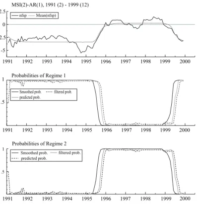
Figure 1
1991 1992 1993 1994 1995 1996 1997 1998 1999 2000 -5
-2.5 0 2.5
MSI(2)-AR(1), 1991 (2) - 1999 (12)
nfsp Mean(nfsp)
1991 1992 1993 1994 1995 1996 1997 1998 1999 2000 .5
1 Probabilities of Regime 1
Smoothed prob. filtered prob. predicted prob.
1991 1992 1993 1994 1995 1996 1997 1998 1999 2000
.5 1
Probabilities of Regime 2
The top panel of figure 1 plots the primary deficit in Brazil in percentage of GDP. The bottom panel plots the smoothed probability that the process was in regime 2 at each date in the sample, that is,p(st = 2|y1, ..., yT;θ) is plotted as a
function of t. This inference uses the full sample of observations (y1, ..., yT) and
the maximum likelihood estimates of parameters ˆθ to draw inferences about the regime of the deficit process at each period. We can determine the dates at which the deficit process had switched between regimes based onp(st= 2|y1, y2, ..., yT)>
0.5. In fact, by our estimates the switches between states are infrequent. We have only two changes in regime. The fiscal policy was in an expansionary state (that is, in state 2) from 1995 to 1999, and was in a consolidation state (state 1) from 1991 to 1995.
The consolidation state from 1991-1995 is due basically to three facts. The first, is the effect of inflation on the real value of the expenditures. As observed before, some funds could be made available later than the established in the bud-get, implying a loss in real terms. The revenues, on the other hand, were more protected since the taxes were indexed to past inflation. Second, effective adjust-ments in spending were made. One example is the fact that transfers to the public enterprieses were virtually eliminated. Third, the recovery of the economy after 1993 had positive effects on the revenue.
The expansionary state from 1995-1999 is due, on the other hand, to two factors. First, an increase in the transfers to states and municipalities. Second, a discretionary increase in expenditures. The Constitution did not determined as mandatory the adjustment of some spendings but they were even though increased.
4.
Size and composition of fiscal adjustments
The next question to be answered is whether the size and the composition of fiscal consolidation influences its probability of success.
Giavazzi and Pagano (1990) believe that a sharp fiscal contraction could be expansionary, based on expectational effects of fiscal contractions. If large fiscal contractions signal lower future tax burdens, this could increase the expected lifetime disposable income, and in turn increase consumption. Besides, Giavazzi and Pagano (1995) argue that the responses of private consumption are more likely when changes in fiscal policy are large and persistent.
spending (e.g., maintenance of public structure) cannot be postponed forever. On the other hand, cuts in welfare obtained by a change in the eligibility criteria for transfer payments have permanent effects. Therefore, even if the two types of spending cuts have the same magnitude, the lasting effects are different. Second, governments that are able to cut the politically more delicate components of the budget (public employment, social security, welfare programs) may signal that they are more committed to a serious fiscal adjustment.
Alesina and Perotti argue that in successful adjustments, 73% of the adjust-ment is on the spending side while in unsuccessful adjustadjust-ments only 44% of the adjustment is on the expenditure side. They still call attention for the differ-ences in composition of types of spending and sources of revenue. Concerning the spending side in unsuccessful episodes more than 66% of the cuts are in public investment while in successful cases only 20% of the cuts are in capital spending. The important difference is that in successful cases the largest cuts are in transfers and wages (together they represent around 50% of the total expenditures cuts). In unsuccessful cases government wages remain practically unchanged.
Successful adjustments, therefore, imply cuts that include especially the polit-ically sensitive parts of the budget. Unsuccessful adjustments priviledges cuts in public spending. One reason for this choice is that to the eyes of the voters cuts in public spending are less visible than cuts in wages and pensions.
Concerning the composition of tax increases, in successful adjustments tax increases are concentrated in business and indirect taxes. In successful cases, the tax increase is not concentrated in any category.
McDermott and Wescott (1996) also obtain the same results. Fiscal consolida-tions, based on cuts on the expenditure side, especially transfers and government wages, are more likely to succeed in reducing the debt ratio. However, contrary to Alesina and Perotti, they believe that the differences in composition of adjustment are as impressive as the differences in size. The greater the magnitude of the fiscal consolidation, the more likely it is to be successful because it appears as more credible.
Table 4
Public Sector Operations (in percent of GDP)
1993 1994
Revenue 31.29 33.04
Tax Revenue 15.60 18.19
IPI 2.44 2.12
Income Tax 3.89 3.65
Social Security Contributions 5.47 4.84
Expenditures 35.76 29.92
Wages 13.77 13.00
Goods and Services 6.86 3.73 Pensions and Welfar 5.57 5.37
Subsidies 2.64 2.91
Transfers 0.51 0.64
Public Investment 5.97 4.06
Source: Secretaria de Pol´ıtica Econˆomica , Minist´erio da Fazenda.
The following aspects of table 4 call attention:
• In 1994 we observe an episode of fiscal consolidation in Brazil that is not successful but that is characterized by a broader adjustment on the expen-diture side, contrary to what is observed in most unsuccessful cases where the adjustment is more on the spending side.
• Transfers and wages are virtually unaltered as would be expected in unsuc-cessful adjustments.
• Expenditures with goods and services as well as with investments suffer large cuts as would be expected in unsuccessful adjustments.
• Tax increase is spread among all components as would be expected in un-successful episodes.
Therefore, the Brazilian fiscal adjustment in 1994 matches perfectly the profile of a standard unsuccessful adjustment in what concerns differences in composition of types of spending and sources of revenue. However, the matching does no longer exist when the size of the adjustment is considered.The largest part of the adjustment was observed on the spending side as in successful cases.
5.
Conclusions
the determination of periods of fiscal consolidation and fiscal stimulus. Using an informal criteria that includes the magnitude of the adjustment as well as the number of periods that are considered for the changes, 1994 is classified as a consolidation year, 1995 is classified as an expansion year and 1999 is classified as a consolidation year. When the primary deficit process is modeled as a Markov chain, there is a change in regime in 1995 (contraction to expansion) and in 1999 (expansion to contraction). The second one is the importance of the composition of fiscal adjustments for their success, defined as a declining debt to GDP ratio.The 1994 consolidation can not be considered successful since after that period the debt to GDP ratio has grown continuously. The adjustment can be characterized as a type 2 adjustment (Alesina and Perotti, 1997) in the sense that cuts were made mainly in public investment, while government wages and transfers remained almost unchanged. This type of adjustment usually has a low likelihood of being a success.
In the analysis we have focused on the government as a whole. For further research it would be interesting to investigate the role of local governments during major fiscal adjustments. Evidence on the size and composition of adjustments by states and municipalities would be very helpful to understand the low rate of success of fiscal consolidations in Brazil.
References
Alesina, A. & Perotti, R. (1997). Fiscal adjustments in OECD countries: Compo-sition and macroeconomic effects. IMF Staff Papers, 44(2):210–248.
Bevilaqua, A. S. & Werneck, R. L. F. (1997). Fiscal impulse in the brazilian economy, 1989-1996. Discussion Paper n. 379, PUC-RIO.
Blanchard, O. (1990). Suggestions for a new set of fiscal indicators. OECD Eco-nomics and Statistics Department, Working Paper n. 79.
Chand, S. K. (1999). Mensura¸c˜ao do impulso fiscal e seu impacto. In e A. Cheasty (Org.), M. I. B., editor,Como Medir O D´eficit P´ublico: Quest˜oes Anal´ıticas e Metodol´ogicas. Secretaria do Tesouro Nacional.
Faria, L. V. (1996). Pol´ıtica Fiscal: O D´eficit ´E Tudo? Conjuntura Econˆomica.
ed. by O. Blanchard and S. Fischer (Cambridge, Massachusetts: MIT Press), 75-111.
Giavazzi, F. & Pagano, M. (1995). Non-keynesian effects of fiscal policy changes: International evidence and the swedish experience. NBER Working Paper, n. 5332 (Cambridge, Massachusetts: National Bureau of Economic Research.
Hamilton, J. D. (1994). Time Series Analysis. Princeton University Press.
McDermott, J. & Wescott, R. F. (1996). An empirical analysis of fiscal adjust-ments. IMF Staff Papers, 43(4):725–753.
Muriel, B. (1996). Determinaci´on de los efectos del producto e inflaci´on sobre el nivel de recaudaciones. Departamento de Economia, PUC-Rio, mimeog.