A straightforward multiallelic significance test for the Hardy-Weinberg equilibrium law

A straightforward multiallelic significance test for the Hardy-Weinberg

equilibrium law

Marcelo S. Lauretto

1

_{, Fabio Nakano}

2

_{, Silvio R. Faria Jr}

3

_{, Carlos A.B. Pereira}

3

_{and Julio M. Stern}

3 1

Escola de Artes, Ciências e Humanidades, Universidade de São Paulo, São Paulo, Brazil.

2

_{Instituto de Química, Universidade de São Paulo, São Paulo, Brazil.}

3

_{Instituto de Matemática e Estatística Universidade de São Paulo, São Paulo, Brazil.}

Abstract

Much forensic inference based upon DNA evidence is made assuming Hardy-Weinberg Equilibrium (HWE) for the genetic loci being used. Several statistical tests to detect and measure deviation from HWE have been devised, and their limitations become more obvious when testing for deviation within multiallelic DNA loci. The most popular meth-ods-Chi-square and Likelihood-ratio tests-are based on asymptotic results and cannot guarantee a good perfor-mance in the presence of low frequency genotypes. Since the parameter space dimension increases at a quadratic rate on the number of alleles, some authors suggest applying sequential methods, where the multiallelic case is re-formulated as a sequence of “biallelic” tests. However, in this approach it is not obvious how to assess the general evidence of the original hypothesis; nor is it clear how to establish the significance level for its acceptance/rejection. In this work, we introduce a straightforward method for the multiallelic HWE test, which overcomes the aforemen-tioned issues of sequential methods. The core theory for the proposed method is given by the Full Bayesian Signifi-cance Test (FBST), an intuitive Bayesian approach which does not assign positive probabilities to zero measure sets when testing sharp hypotheses. We compare FBST performance to Chi-square, Likelihood-ratio and Markov chain tests, in three numerical experiments. The results suggest that FBST is a robust and high performance method for the HWE test, even in the presence of several alleles and small sample sizes.

Key words:Hardy-Weinberg equilibrium, significance tests, FBST. Received: November 4, 2008; Accepted: May 25, 2009.

Introduction

The Hardy-Weinberg law is one of most important principles in population genetics, and establishes a direct relationship between allele and genotypic proportions in a population. This law states that in a large population of panmictic dioecious organisms with non-overlapping gen-erations, the allelic and genotypic frequencies at a locus will stay unchanged, provided that migration, mutation, and natural selection do not affect that locus. When these conditions hold, it is said that the locus is under Hardy-Weinberg Equilibrium (HWE).

This principle was discussed independently by Yule, Pearson and Castle (between 1902 and 1904), for some par-ticular allele frequencies (see references in Crow and Ki-mura, 1972). In 1908, Godfrey Hardy presented the general principle for two alleles (Hardy, 1908). This principle was called Hardy’s law for 35 years, until Stern (1943) called at-tention to an article of Weinberg (1908) showing the same

principle at the same time and demonstrating its validity for multiple alleles (Crow, 1999).

Since its postulation, several results in population ge-netics and much forensic inference based upon DNA evi-dence have been based on the assumption that HWE is valid for the genetic loci of interest. Some statistical tests to de-tect and measure deviation from HWE have been devised, and their limitations have become more obvious when test-ing for deviation within multiallelic DNA loci. The most common approach consists of goodness-of-fits tests, like Chi-square and Likelihood-ratio, which are heavily based on asymptotic results, and can sometimes lead to false re-jection or acceptance of HWE when the sample sizes are small and/or some genotype sample frequencies are very small (Emigh, 1980). Another approach involves exact tests, but is restricted to small dimensions and allele num-bers.

A Bayesian sequential method for multiallelic HWE test was proposed by Pereiraet al.(2006), who suggested reformulating the multiallelic case as a sequence of “bial-lelic” tests. In that work, the central component is the Full Bayesian Significance Test (FBST), an intuitive Bayesian approach which does not assign positive probabilities to

www.sbg.org.br

Send correspondence to Marcelo S. Lauretto. Escola de Artes, Ciências e Humanidades, Universidade de São Paulo, Rua Arlindo Béttio 1000, Ermelino Matarazzo, 03828-000 São Paulo, SP, Brazil. E-mail: marcelolauretto@usp.br.

zero measure sets when testing sharp hypotheses (Pereira and Stern, 1999). Although the sequential method avoids the quadratic increase of parameter space dimension with respect to the number of alleles, it is not obvious how to as-sess the general evidence of the original hypothesis; nor is it clear how to establish the significance level for its accep-tance or rejection (see DeGroot, 1970).

In this work, we propose a method for the multiallelic HWE test, based on the FBST. FBST has many theoretic and practical advantages over other approaches, and it has shown to be robust in several high-dimensional problems (Laurettoet al., 2008).

Background

In this section we introduce some notations, and the Hardy-Weinberg Equilibrium (HWE) formula. Let us con-siderkallelesA1,A2, ...,Akin alocus. The main interest is to

assess the population relative frequencies of the genotypes

AiAj(i, j= 1, 2, ...,k) which we denote bypij. As usual in the

literature (see Hardy, 1908), we assume that the allele fre-quencies do not depend on sex and thus are symmetric, that is,AiAjis equivalent toAjAiandpij=pji. Therefore, the

pa-rameter of interest is the (lower triangular) matrix of geno-type proportions:

q= (qij), withqii=pii,qij= 2pijfor 1£j£i£k.

We denote byp1,p2, ...,pkthe (unknown) population

frequencies of alleles A1, A2, ..., Ak, with pi ³ 0 and pi

i k

=

å

₁ =1. When the locus is under HWE, the genotype proportions are as follows:

q_ii =p_i2; q_ij =2p p_{i j},1£ £ £j i k. (1)

In order to test the HWE in a locus, one considers a sample ofnindividuals drawn randomly from the popula-tion. Such a sample can be presented as the arrayx, whose elementsxij, 1£ £ £j i k, are counts of genotypesAiAj. The

sample sizenisn j i xij k

=

å

_{£ =1} , and the sample frequency of

allele Ai is ni j xij x i

ji j i k

=

å

₌₁ +

å

₌ . Note that

å

ini =2 ,n

since all loci have two alleles and this sum is the number of alleles in the whole sample. The sample proportion of allele

Ai, ~pi, is given by

~_p n _. n i

i

=

2 (2)

Assuming that each individual genotype does not de-pend on remaining individuals in the same generation, we can consider that the genotype frequencies xij follow a

multinomial distribution with unknown parameterq,

P x n

x ij x ij j i k ij ( | ) ! !.

q = q

£ =

Õ

1

(3)

Testing Procedures

In this section we present three tests used in our com-parative study. These and other approaches are described by Emigh (1980), Guo and Thompson (1992), Hernández and Weir (1989) and Montoya-Delgadoet al.(2001).

Chi-square goodness-of-fit test

This test involves calculating the sample chi square value, c2 2 1 = -£ =

å

(x E ) ,

E ij ij ij j i k (4) with

E np n

n i k

E np p n n

n j i ii i

i

ij i j

i j

= = =

= = <

~ _{( , , ),} ~ ~ ₍ 2 2 1 4 1 2 1 2 K ).

Under HWE, this quantity has a chi-square distribu-tion withk(k– 1)/2 degrees of freedom.

The Chi-square goodness-of-fit test with continuity correction involves calculating the previous statistics, with the subtraction in each term of a correction constantc:

c2

2

1

= -

-£ =

å

(|x E | )c .

E ij ij ij j i k (5)

Usuallyc= 0.5 is the value chosen.

Likelihood-ratio tests

The likelihood function, given a sample, follows di-rectly from the multinomial distribution presented in Eq. (3). A Likelihood-ratio test is constructed by compar-ing the likelihood maximized under the hypothesis,L0, with

the maximum likelihood,L1, not constrained by the

hypoth-esis. For HWE we have

L n

n x

x L n

p x p n ij x ij j i k i x ii i k ij ii 1 1 0 2 1 2 = = £ = =

Õ

Õ

! !, ! ~ !

( ~i j x ij j i p x ij ~ ) ! . <

Õ

(6)

with the sample allelic frequencies, ~pi, given by Eq. (2). The test statistic

G L

L

2 0

1 2

= - æ è çç ö_ø÷÷

ln (7)

is asymptotically distributed as a chi-square distribution withk(k– 1)/2 degrees of freedom.

Markov Chain Monte Carlo (MCMC) method

samples that have the same allelic counts as the observed data.

Under HWE and conditional on sample allele counts,

n1,n2, ...,nk, the probability of obtaining the samplexis (see

Levene, 1949):

Pr( | , , ) !

( )! .

x n n

n n n x k i i ij j i xij j i 1 2 2

K ₌

Õ

å

Õ

<

< ₍₈₎

Given the datax, the test evaluates

P y

y

=

ÎÃ

å

Pr( ), (9)

whereà ={ :Pr( ) Pr( ),y y £ x xÎG0}and

G0 =G( )x ={y:yhas the same allele counts as doesx}. (10)

The MCMC algorithm is performed in order to esti-mate the probabilityPin E. (9). Rejection or acceptance of the null hypothesis depends on whetherPis smaller than a pre-specified significance levela.

Methods

The Full Bayesian Significance Test (FBST)

The Full Bayesian Significance Test (FBST) was pro-posed by Pereira and Stern (1999) as a coherent and intu-itive Bayesian test. It assumes that the hypothesis,H, is defined as a subset defined by inequality and equality con-straints:

H _{H H} g h

n

: { | ( ) ( ) },

.

qÎ = qÎ q £ Ù q =

Í Â

Q Q Q

Q

for and

0 0

(11)

For simplicity, we often useHforQH. FBST is

par-ticularly focused on precise hypotheses: i.e., dim(QH) < dim(Q). In this work, fx( )q denotes the poste-rior probability density function, given the observationx. Bold0and1denote vectors of appropriate dimensions.

For the HWE test, the parametric space consists of all arrays of genotype proportions

{

}

Q = q=(q_ij), £ £ £ |q³ Ù

å

_{£ =} q_ij = . j i

k j i k

1 0 ₁ 1 (12)

The space on hypothesis is

{

H p p p p i k

p p j

H k ii i

ij i j

º = Î $ = =

= <

Q q Q q

q | , , , : ( , , ), ( 1 2 2 ₁ 2 K K

}

i),0£p£1,p¢ =1 1 .

(13)

As previously stated, we consider that the genotype frequenciesxfollow a multinomial distribution, given by Eq. (3). Taking as a priori the Dirichlet distribution with pa-rameters (1,1...1),i.e., a uniform distribution, then the a posteriori is a Dirichlet distribution with parameters (x11+ 1,x21+ 1,x22+ 1, ...,xkk+ 1) which is proportional to

the likelihood function (DeGroot, 1970):

f n k

x x ij x ij j i k ij x j i k ij ij ( ) ( ) ( )

q = + q q

+ µ £ = £ =

Õ

Õ

G G 1 1 1 (14)

The computation of the evidence measure used on the FBST is performed in two steps:

1.The optimization stepconsists of finding the maxi-mum (supremaxi-mum) of the posterior under the null hypothe-sis,q* _{=arg sup ( ),}q * _{= (}q*₎

H fx f fx .

2.The integration stepconsists of integrating the pos-terior density over the Tangential Set,T, where the poste-rior is higher than anywhere in the hypothesis,i.e.,

{

}

Ev H T x f d

T f f

x T

x

x

( ) Pr( | ) ( ) ,

: ( )

= Î =

= Î >

ò

q q q

q q

where

Q

(15)

Ev(H) is the evidence againstH, andEV(H) = 1 –Ev(H) is the evidence supporting (or in favor of)H. For a better un-derstanding of this evidence measure, Figure 1 illustrates two examples in the biallelic case, showing the null and tan-gential sets (QHandT). Sinceq21= 1 –q11–q22, the

para-metric space is fully defined by homozygote proportions,

q11andq22. The parameter space corresponds to the area

in-side the triangle. Sample genotype counts forA11,A21,A22

andEv(H) are also shown in each graph. Marker ‘*’ repre-sents the pointq*

of maximum a posteriori density in the constrained spaceQH, and the level curve tangent toq*

cor-responds toTfrontier. Intuitively, if the hypothesis set is in

a region of “low” posterior density (as in the example 1), thenTis “heavy” and thereforeEv(H) is “large” (@0.91), meaning “strong” evidence againstH. On the other hand, as illustrated by the example 2, if hypothesis set is in a region of “high” posterior density, then T is a “small” set, and henceEv(H) is “small” (@0.36), meaning “weak” evidence againstH.

For HWE test, the pointq* _{=arg sup ( )}q

H fx is given as follows.

Rewriting the posterior pdf under HWE, we have:

fx H pi p p

x i j x j i i k ii ij

( | )q µ ( )

<

=

Õ

Õ

2

1

2 . (16)

Taking its logarithm,

l f H n p

n p p

x x ii i

i k

ii i j

j i

( ) log ( | ) log

log( )

q º q µ +

= = <

å

å

2 2 1

h ni pi

i k

log2 log ,

1

+

=

å

(17)

whereni xij j xji k j

i

=

å

₌₁ +

å

₌₁ , andhis the sum of sample heterozygote frequencies,h=

å

_{j i<} xii.

By the constraint i pi k

=

=

l h n p

n n p

x i i

i k

k j j

j k

( ) log log

log log

q µ + +

-æ è = -=

-å

å

2 1 1 1 1 1 ç ç ö ø ÷ ÷. (18)

The gradients oflx(q) are given by:

¶ ¶ l p n p n p x i i i k j j k µ -=

-å

1 1 1 (19)

Hence, the optimal point under HWE is given by the

vector p p pk

* * *

( , , )

= ₁ K _{-1 which satisfies:}

Ap b A

n n n n

n n n n

n n n n

k

k

k k k k

= = + + + æ è ç - - -;

1 1 1

2 2 2

1 1 1

K

K

M M O M

K ç ç çç ö ø ÷ ÷ ÷ ÷÷ = ì í ï ï î ï ï ü ý ï ï þ ï ï -; . b n n nk 1 2 1 M . (20)

Summing over all constraints and after some algebra, we obtain the following solution:

p p p n

n i k

i i

i

* * ~

, , ,

= = = =

2 1K .

The computation ofq* _from

p* follows from Eq. (1).

The integration step may be performed by generating a set ofMpoints {_q( )1 ,_q( )2 , ,_{K q}( )M}_{with a Dirichlet} distri-bution with parameter (x11+ 1,x21+ 1,x22+ 1, ...,xkk+ 1)

and computing the percentage of points with posterior den-sity greater thanf*:

q( )_{~ ( , , , ), , , ,}

( ) r

kk

x x x r M

Ev H

Dirichlet ₁₁+1 ₂₁+1K +1 =1 2K

=

å

=I f > f

M x

r r

M

( (_q( )) *) 1

(21)

whereI(stat) = 1 ifstatis true and 0 otherwise. A more pre-cise and efficient Monte Carlo method for the integration step is presented by Laurettoet al.(2003).

As with any significance test, this procedure requires the choice of a threshold level,t, for acceptance/rejection of the hypothesis at a significance levela. Several alterna-tive methods have been developed for establishing this threshold:

• An empirical power analysis, developed by Stern and Zacks (2002) and Laurettoet al.(2003), pro-vides critical levels that are consistent and also ef-fective for small samples.

• A threshold based on reference sensitivity analysis and paraconsistent logic is given by Stern (2004). • Pereiraet al.(2008) relates the e-value threshold to

standard p-value thresholds.

• Madrugaet al.(2001) proves the existence of a loss function that renders the FBST a true Bayesian de-cision-theoretic procedure.

• An asymptotically consistent threshold for a given confidence level was given by Stern (2007), and Borges and Stern (2007), which we adopt in this work.

Let us consider the cumulative distribution of the evi-dence value against the hypothesis,V( ) Pr(t = Ev H( )£t), givenq0

, the true value of the parameter. Under appropriate

regularity conditions, for increasing sample size, we can state the following:

IfHis false,q0_Ï

H, thenEv(H) converges (in proba-bility) to one, that is,V( )t ®d( )1 .

IfHis true,q0_Î

H, thenV(t), the confidence level, is approximated by the function Q(t, h, t) = Chi2( Chi2 (-1 ))

t-h, t,t , wheret= dim(Q),h= dim(H) and Chi2(df,x) denotes the cumulative chi-square distribution withdfdegrees of freedom.

Hence, to rejectHwith a significance levela, we can sett= - -a

Q 1( , ,t h1 ),i.e., settsuch thatQ t h( , , )t = -1 a.

Results and Discussion

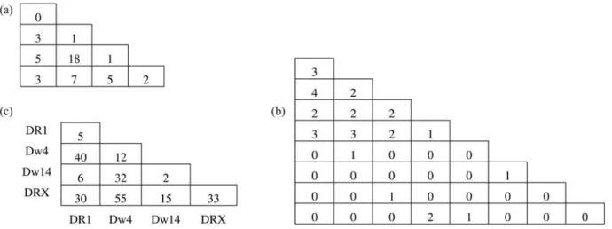
The numerical experiments used in the performance analysis are based on three typical datasets. Two examples consist of simulated data used in the literature as benchmarks for comparing the performance of competing methods, while the third example is from a real dataset. These examples are presented in Figure 2, as lower triangu-lar matrices containing genotype frequencies. The first example is taken from Louis and Dempster (1987) and con-sists of a sample of size 45 of genotype frequencies distrib-uted in four alleles. The second example is given by Guo and Thompson (1992) and consists of a sample of size 30 of simulated genotype frequencies simulated under HWE with underlying allele frequencies (0.2, 0.2, 0.2, 0.2, 0.05, 0.05, 0.05, 0.05). The third example is from a rheumatoid arthritis (RA) study performed by Wordsworth et al.

(1992), where two hundred and thirty RA patients were genotyped for the HLA-DR locus. The DR4 allele was sub-divided into Dw4, Dw14 and other subtypes. DRX repre-sents all non-DR1, non-Dw4, non-Dw14 alleles. This example is used by Chen and Thomson (1999) as a bench-mark.

Our main interest is to compare the error convergence of FBST and other methods presented in this work (MCMC, Chi-square and Likelihood-ratio) for increasing

sample sizes. For each sample sizenÎ{ ,30 50 100 200 we, , }, simulated two collections of 100 samples. The first collec-tion consists of samples drawn under HWE,i.e., each sam-ple is drawn with a multinomial distribution with parame-ters (n, q*

), with q* _q q

arg max ( )

= _ÎH f_x . The second

collection consists of samples drawn with a multinomial distribution with parameters (n,q( )h

), whereq( )h

is drawn under the posterior distribution. That is, each sampling iter-ation is performed in two steps:

a) draw q( )h _{~ ( , , , )}

kk

x x x

Dirichlet ₁₁+1 ₂₁+1K +1_, wherexij(1£j£i£k) are the frequencies in the original

dataset; and

b) drawX( )h ~Multinomial( ,n q( )h ).

The Type I error (rejection rate of a true hypothesis) is estimated by the proportion of samples in collection 1 such that HWE is rejected, and the Type II error (acceptance rate of a false hypothesis) is estimated by the proportion of sam-ples in collection 2 such that HWE is accepted. The perfor-mance criterion used in this work is the average error,i.e., the average of Types I and II error rates. Two standard sig-nificance levels,a Î{0.01, 0.05}, were used to calibrate the asymptotic acceptance/rejection threshold of each method.

A variability measure for the errors was obtained by performing 10 batches of simulations and computing the mean and standard deviation of average errors across the batches.

Figure 3 presents the average errors for FBST, MCMC, Chi-square (with continuity correction) and Like-lihood ratio for simulated data based on examples 1, 2 and 3. The bar height represents the mean of average errors, and the vertical line on the top of each bar is the error bar, repre-senting the mean±one standard deviation of average er-rors.

For simulated data based on examples 1 and 3, the best competitors are FBST and Likelihood-ratio test, while for simulated data based on example 2, the best competitors

are FBST and MCMC. In every case, we notice that FBST is always the best competitor (especially for small sample sizes,n£100) or is very close to it.

These numerical results suggest that FBST is more stable than the competitors discussed in this paper, in the sense that it has good comparative performance for differ-ent datasets and allele numbers.

Final Remarks

We have introduced a simple and straightforward procedure for testing deviance from Hardy-Weinberg Equi-librium (HWE) in the presence of several alleles. This pro-cedure was implemented in C language, and integrated into a system for parentage testing developed with FAPESP support, where it is applied in the selection of loci to be used for parentage testing. Further details of this project can

be found at http://watson.fapesp.br/PIPEM/Pipe13/genet1. htm. Currently, the routine is available by request to the corresponding author.

Acknowledgments

The authors are grateful for the support of EACH-USP, IQ-EACH-USP, IME-EACH-USP, Coordenação de Aperfeiçoa-mento de Pessoal de Nível Superior (CAPES), Conselho Nacional de Desenvolvimento Científico e Tecnológico (CNPq) and Fundação de Apoio à Pesquisa do Estado de São Paulo (FAPESP).

References

Borges W and Stern JM (2007) The rules of logic composition for the Bayesian epistemic e-values. Logic J IGPL 15:401-420.

Figure 3- Average error rates for FBST, MCMC, Chi-square and Likelihood-ratio for simulated data based on examples from Louis and Dempster

Chen JJ and Thomson G (1999) The variance for the disequilib-rium coefficient in the individual Hardy-Weinberg test. Bio-metrics 55:1269-1272.

Crow JF and Kimura M (1972) An Introduction to Population Ge-netics Theory. Harper & Row, New York, 591 pp.

Crow JF (1999) Hardy, Weinberg and language impediments. Ge-netics 152:821-825.

DeGroot MH (1970) Optimal Statistical Decisions. Wiley, New York, 489 pp.

Emigh TH (1980) A comparison of tests for Hardy-Weinberg equilibrium. Biometrics 36:627-642.

Guo SW and Thompson EA (1992) Performing the exact test of Hardy-Weinberg proportion for multiple alleles. Biometrics 48:361-372.

Hardy GH (1908) Mendelian proportions in a mixed population. Science 28:49-50.

Hernández JL and Weir BS (1989) A disequilibrium coefficient approach to Hardy-Weinberg testing. Biometrics 45:53-70. Lauretto MS, Pereira CAB, Stern JM and Zacks S (2003) Full

Bayesian significance test applied to multivariate normal structure models. Braz J Probabil Stat 7:147-168.

Lauretto MS, Pereira CAB and Stern JM (2008) The full Bayesian significance test for mixture models: Results in gene expres-sion clustering. Genet Mol Res 7:883-897.

Levene H (1949) On a matching problem arising in genetics. Ann Math Stat 20:91-94.

Louis EJ and Dempster ER (1987) An exact test for Hardy-Weinberg and multiple alleles. Biometrics 43:805-811. Madruga M, Esteves LG and Wechsler S (2001) On the

Baye-sianity of Pereira-Stern tests. Test 10:291-299.

Montoya-Delgado LE, Irony TZ, Pereira CAB and Whittle MR (2001) An unconditional exact test for the Hardy-Weinberg

equilibrium law: Sample-space ordering using the Bayes factor. Genetics 158:875-883.

Pereira CAB, Nakano F, Stern JM and Whittle MR (2006) Genu-ine Bayesian multiallelic significance test for the Hardy-Weinberg equilibrium law. Genet Mol Res 5:619-631. Pereira CAB and Stern JM (1999) Evidence and credibility: Full

Bayesian significance test for precise hypotheses. Entropy J 1:69-80.

Pereira CAB, Stern JM and Wechsler S (2008) Can a significance test be genuinely Bayesian? Bayesian Anal 3:79-100. Stern C (1943) The Hardy-Weinberg law. Science 97:137-138. Stern JM and Zacks S (2002) Testing the independence of Poisson

variates under the Holgate bivariate distribution. The power of a new evidence test. Stat Probabil Lett 60:313-320. Stern JM (2004) Inconsistency analysis for statistical tests of

hy-pothesis. In: López-Díaz M and Gil MA (eds) Soft Method-ology and Random Information Systems. Springer, New York, pp 567-574.

Stern JM (2007) Cognitive constructivism, eigen-solutions and sharp statistical hypotheses. Cybernet Hum Knowing 14:9-36.

Weinberg W (1908) Über den Nachweis der Vererbung beim Menschen. Jahresh Wuertt Verh Vaterl Naturkd 64:369-382.

Wordsworth P, Pile KD, Buckley JD, Lanchbury JSS, Ollier B, Lathrop M and Bell JI (1992) HLA heterozygosity contrib-utes to susceptibility to rheumatoid arthritis. Am J Hum Genet 51:585-591.

Guest Editor: José Carlos Merino Mombach