Customer Clustering in the Insurance Sector by Means of Unsupervised Machine Learning Techniques

i

Customer Clustering in the Insurance Sector by

Means of Unsupervised Machine Learning

Thies Bücker

An internship report

i Title: Customer Clustering in the Insurance Sector by Means of

Unsupervised Machine Learning Techniques

Student

Thies Bücker

MAA

201

ii

NOVA Information Management School

Instituto Superior de Estatística e Gestão de Informação

CUSTOMER CLUSTERING IN THE INSURANCE SECTOR BY MEANS OF

UNSUPERVISED MACHINE LEARNING

by

Thies Bücker

Internship report presented as partial requirement for obtaining the Master’s degree in Advanced Analytics.

Advisor: Mauro Casteli

iii

ACKNOWLEDGEMENTS

I would like to express my gratitude to my supervisor, Mauro Casteli, of Nova Information

iv

ABSTRACT

Clustering is one of the most frequently applied techniques in machine learning. An overview of the most comon algorithms, problems and solutions is provided in this report. In modern times,

customer information is a curtail success factor in the insurance industry. This work describes a way how customer data can be leveraged in order to provide useful insights that help driving business in a more profitable way. It is shown that the available data can serve as a base for customer

segmentation on which further models can be built upon. The customer is investigated in three dimensions (demographic, behavior, and value) that are crossed to gain precise information about customer segments.

KEYWORDS

v

INDEX

1.

Introduction ... 1

2.

Motivation ... 2

3.

Clustering ... 3

3.1. Definition and Application ... 3

3.1.1.

Definition ... 3

3.1.2.

Fields of Research ... 4

3.1.3.

Clustering Approaches ... 4

3.2. Hierarchical Clustering ... 5

3.2.1.

Dendrogram ... 6

3.2.2.

Similarity Measures ... 7

3.2.3.

Metrics ... 8

3.2.4.

Divisive Algorithms ... 9

3.3. Partitional Clustering ... 10

3.3.1.

K-Means Algorithm ... 10

3.3.2.

Advantages and Disadvantages of K-Means ... 10

3.3.3.

Outlier Detection ... 12

3.3.4.

Initializations for K-Means ... 15

3.3.5.

Number of Clusters ... 20

3.4. Cluster validation & Similarity Measures ... 21

3.4.1.

External Validation Techniques ... 22

3.4.2.

Internal Validation Techniques ... 24

4.

Customer Clustering For an insurance ... 29

4.1. Data Sources ... 29

4.2. Segmentation ... 31

4.2.1.

Demographic Segmentation ... 32

4.2.2.

Behavior Segmentation ... 37

4.2.3.

Value Segmentation ... 45

4.3. Final Deliverable ... 54

5.

Results and Limitations ... 56

6.

Bibliography ... 58

7.

Appendix ... 63

vi

7.2. Correlation Matrix for Demographic Segmentation ... 97

7.2.1.

Section 1 of the demographic correlation matrix ... 99

7.2.2.

Section 2 of the demographic correlation matrix ... 100

7.2.3.

Section 3 of the demographic correlation matrix ... 101

7.2.4.

Section 4 of the demographic correlation matrix ... 101

7.2.5.

Section 5 of the demographic correlation matrix ... 102

7.2.6.

Section 6 of the demographic correlation matrix ... 102

7.3. Profiling of Demographic segments ... 102

7.4. Profiling of Behavior segments ... 106

vii

LIST OF FIGURES

Figure 1 - Dendrogram example... 6

Figure 2 - Similarity measures ... 7

Figure 3 - Creation of the CAR ... 30

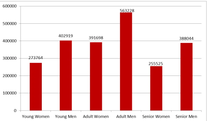
Figure 4 - Number of customers in demographic segments ... 35

Figure 5 - Age distribution of demographic segments ... 35

Figure 6 - Scatter plot of the first two principal components for the demographic

segmentation ... 37

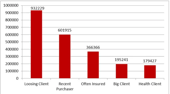
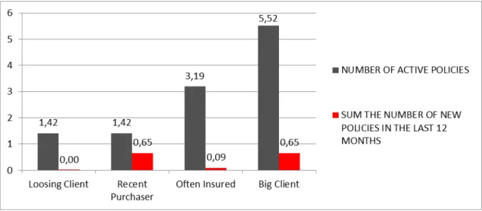
Figure 7 - Number of customers in behavior segments ... 42

Figure 8 - Number of years since last purchase ... 42

Figure 9 - Number of new policies (12 month) vs. number of total policies ... 43

Figure 10 - Number of contracts as an insured person ... 44

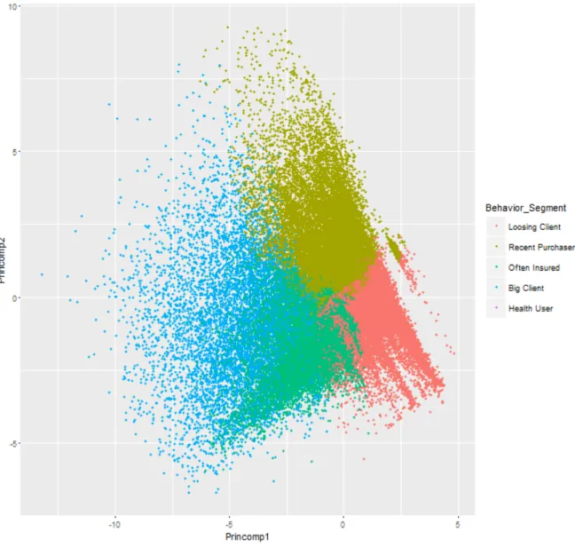
Figure 11 - Scatter plot of the first two principal components for the behavior segmentation

... 45

Figure 12 - Number of clients in value segments ... 50

Figure 13 - Average current value of financial products per client... 51

Figure 14 - Average technical margin by value segment ... 51

viii

LIST OF TABLES

Table 1 - Definitions of clustering ... 3

Table 2 - Classical outlier definitions ... 13

Table 3 - Translation from Event/Non-Event to True/False Positive/Negative. Correctly

classified are marked in green, while incorrectly classified observations are marked in

orange. ... 22

Table 4 - Categories and key words for topic extraction from phone call notes ... 31

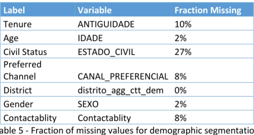
Table 5 - Fraction of missing values for demographic segmentation ... 33

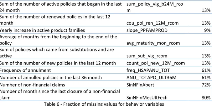
Table 6 - Fraction of missing values for behavior variables ... 39

Table 7 - Correlations among behavior variable ... 40

Table 8 - Fraction of missing values among value variables ... 47

Table 9 - Correlation among value variables... 49

Table 10 - Overview of the demographic correlation matrix ... 98

Table 11 - First section of the demographic correlation matrix ... 99

Table 12 - Second section of the demographic correlation matrix ... 100

Table 13 - Third section of the demographic correlation matrix ... 101

Table 14 - Fourth section of the demographic correlation matrix ... 101

Table 15 - Fifth section of the demographic correlation matrix ... 102

1

1.

INTRODUCTION

The Master’s degree in Advanced Analytics contains a praxis phase, which can be done in form of an internship with a company. For this report Accenture has been chosen to be the partnering company for the internship. Because of the partnership between Accenture and Nova IMS it is ensured that the content of the internship fits the topics of the university course. Due to that reason the internship has been held in the Advanced Analytics department of Accenture in Lisbon between the 26.10.15 and 22.04.16. The main reason for the internship is to show the student relevant topics in the area of advanced analytics while improving his practical hard skills and soft skills.

2

2.

MOTIVATION

In the past years the environment for business has changed and is changing on an accelerating velocity. Due to globalization new competitors emerge and due to modern communication technology and media, prices and services are comparable easily, cost-efficiently and fast. Enterprises that ran their business model successfully for years, might face new challenges and obstacles because of quickly changing customer behavior or technologies that are applied by a competitor. These changes increase the pressure on companies of all industries. One of the industries that is effected most by these changes is the insurance industry. In this particular industry the number of clients of a company has is one of the main success drivers and has a major impact on the profitability of the company. And thus, customer retention becomes one of the key concerns of insurance businesses in our days. The cost of attracting new customers is much higher than the cost of retaining the clients that are already related to the company. For this reason it is crucial to the enterprises to keep their clients active. In order to do so, clients must be managed in a customized way that suits their needs and makes them profitable to the enterprise. For an insurance it is indispensable to precisely know its clients. Clients cannot all be treated in the same manner, but must be handled in a tailored way. In pursuance of that it is necessary for a company to know its customers. In many businesses information about the client is rarely used, even though it is available. One way of getting to know the customer base and identifying possible management strategies is clustering. Clustering provides the applicant with a sense of what a typical client is. Further it equips the researcher with a solid understanding of different customer segments. Based on these segments specific strategies can be worked out to target the customer in a more specific, and so more successful and efficient way.

3

3.

CLUSTERING

Because clustering has been discussed widely in literature over the past decades, a variety of definitions can be found while researching about clustering. That is why it should be started by giving an overview of definitions. This goes together with a brief description of the fields in which clustering is applied. Later on different clustering branches will be described, compared and common problems will be explained.

3.1.

D

A

Clustering is not one specific algorithm, but rather a group of algorithms with similar goals. This section should give conclusion about the matter of clustering, provide an overview of different clustering types, and should give a brief summary of the field in which clustering is applied broadly.

3.1.1.

Definition

The exact definition of clustering varies depending on the researcher and the respective research field and topic. In general clustering is considered a form of unsupervised machine learning (A. Jain, Murty, & Flynn, 1999). In contrast to supervised machine learning, it does not try to approach a target value. However it might be helpful to compare the outcome of clustering algorithm to the real clusters, if available. Specific techniques are described in section External Validation Techniques. The following table provides an overview of different definitions.

Author(s)

Definition

(Jain, Murty, & Flynn, 1999, p.264)

“

Clustering is the unsupervised

classification of patterns (observations,

data items, or feature vectors) into groups

(clusters)

”

(Liu, Li, Xiong, Gao, & Wu, 2010, p.911)

“

dividing a set of objects into clusters such

that objects within the same cluster are

similar while objects in different clusters

are distinct

”

(Rendón et al., 2008, p.241)

“

determine the intrinsic grouping in a set of

unlabeled data, where the objects in each

group are indistinguishable under some

criterion of similarity

”

(A. K. Jain, 2010, p.651)

“

Cluster analysis is the formal study of

methods and algorithms for grouping, or

clustering, objects according to measured

or perceived intrinsic characteristics or

similarity

”

(Likas, Vlassis, & Verbeek, 2003, p.12)

“

defined as a region in which the density of

objects is locally higher than in other

regions

”

4 In essence clustering pursues the objective of identifying groups of data that are similar to data of the same group and less similar to data of other groups. In this work the terms groups, segments, clusters, and classes are used synonymously.

3.1.2.

Fields of Research

Such properties, as described above, are desirable in a wide range of fields. The following list should provide an overview of some of the most relevant fields in clustering:

- Customer Segmentation: To provide companies with potentially interesting insights about their customer, and help them manage different customer segments in different ways. - Human Genetic Clustering: Applies clustering to human genetic data in order to draw

conclusions about population structure (de Hoon, Imoto, Nolan, & Miyano, 2004).

- Medical Imaging: Uses clustering to make similarly behaving structures insight the body visible and interpretable on a monitor.

- Image Segmentation: Clustering is used to detect similar regions in a visual image. This technique is applied in research topics like object recognition, video analysis for self-driving cars, and map creation from satellite images.

3.1.3.

Clustering Approaches

Due to its appeal to many research areas, a variety of different techniques have emerged over time. This section will distinguish some of the main groups of clustering algorithms.

Bottom-up clustering under the use of a similarity measure is called hierarchical agglomerative clustering. Bottom-up means, that each observation starts in a cluster on its own (singleton) and is then merged with the most similar cluster, or observation, to form a bigger cluster. This process ends at the latest when all observations are merged together into one single cluster. The similarity measure is a parameter of the algorithm, and can be chosen, for example, from the list provided in Similarity Measures (Duda, Hart, and Stork 2001).

One advantage of the agglomerative method is, that the distances at which the clusters have been merged can provide useful information. This information can be useful when deciding the number of clusters. Details about how to use these distances are provided in section Dendrogram.

Cimiano, Hotho, & Staab (2004) point out that the difference between agglomerative and divisive approaches is the bottom-up approach (agglomerative) in contrast to the top-down method (divisive). In divisive clustering algorithms all observations start in a single cluster, and are then subdivided into sub clusters, until each observation ends up in a cluster on its own.

5 dimensionality (number of used variables) that is greater than 100, and would result in a number of clusters that “is so large that the data set is divided into uninterestingly small and fragmented clusters” (p.275). This behavior is the reason why polythetic methods find greater response in research. All further described algorithms use the polythetic approach.

Hard clustering is distinct from fuzzy clustering in terms of the membership of an observation to a cluster. While in hard clustering each observation is assigned to one single cluster, it can be assigned to multiple clusters in fuzzy clustering. In fuzzy clustering each observation has a degree of membership to each cluster, so that the association with the segments is relative. Observations that seem to fit better to one cluster have a greater degree of membership for that cluster, than observations that are only weakly associated to a cluster (A. Jain et al., 1999).

One advantage of fuzzy clustering is, that it can be translated to hard clustering by assigning an observation to the cluster with the highest degree of membership. A translating from hard clustering to fuzzy clustering is not possible without further calculations.

Another dimension that differentiates clustering approaches is how the applied algorithm finds its optimum. If it includes a form of random search (stochastic), or if it approaches the optimal value using a step by step deterministic method (A. Jain et al., 1999).

Clustering techniques can also be divided into incremental and non-incremental clustering. Charikar, Chekuri, Feder, and Motwani (2004) define incremental clustering as follows:

for an update sequence of n points in M, maintain a collection of k clusters such that as each input point is presented, either it is assigned to one of the current k clusters or it starts off a new cluster while two existing clusters are merged into one (p.1419)

The condition to split a cluster, and which and when clusters are joined together is subject to the respective implementation. Incremental clustering is used when data sets become so large, that they are too big to be processed at once, and therefore need to be processed observation by observation. In this case it is important to minimize the number of scans through the data set (A. Jain et al., 1999). Non-incremental clustering, in contrast, deals with the whole data set at once. The algorithms that will be presented are non-incremental functions.

3.2.

H

C

Two of the major branches in clustering are hierarchical clustering and partitional clustering. This chapter will give an overview of the most important topics in hierarchical clustering, while the following chapter will do so for the partitional clustering algorithms.

6 Of a divisive approach is spoken, when a top down method is used. In contrast to the agglomerative approach, all observations start in a single cluster and are split based on a similarity measure until clusters cannot be split anymore, because they only consist of a single observation (Cimiano et al., 2004).

3.2.1.

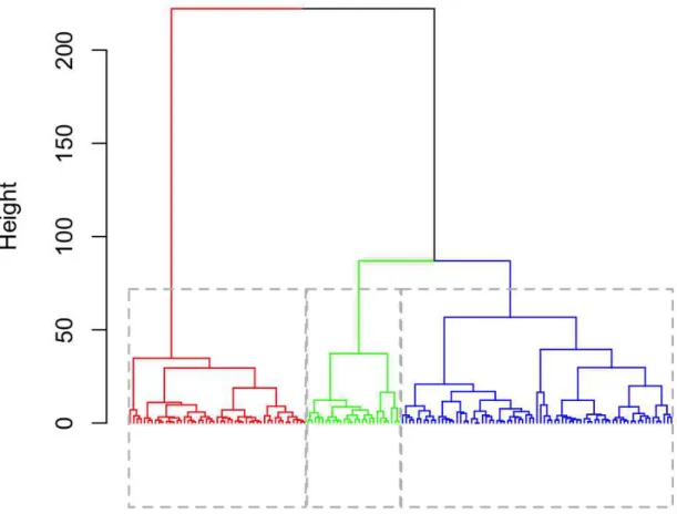
Dendrogram

The procedure agglomerative methods use, merges the most similar observations in an iterative manner. The dendrogram is a chart that gives conclusion about the distance at which two observations/clusters have been joined. It can be used as an indicator for the number of clusters. An example of a dendrogram for a hypothetical clustering task can be seen in Figure 1. The y-axis illustrates the distance at which two observations have been merged. It can be observed, that the two clusters that are joined at last, have a distance greater than 200. In this case the researcher decides to have three final clusters, which have a distance of greater than 75. The next two clusters that would be joined together would be the green and the blue ones.

Note that the dendrogram does not give conclusion about the used similarity measure and metric.

7

3.2.2.

Similarity Measures

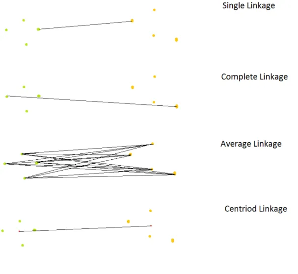
The criteria on which the distances between clusters are evaluated are called similarity measures. These techniques determine how distances are considered and which clusters, or observations, are merged at next. A variety of different similarity measures exist. The most important ones are explained in this section. Figure 2 illustrates how selected similarity measures evaluate the distance between two hypothetical segments.

Figure 2 - Similarity measures

According to (Sibson, 1973) single linkage is one of the oldest methods to measure similarity. It was first proposed by Sneath (1957). In agglomerative clustering methods, single linkage groups the observations/clusters into new clusters that are the most similar. Similarity is defined as the minimal distance between two observations/clusters. Where the distance between two segments is defined as the minimal distance of their observations. This is the distance between the two most similar observations from different clusters. The property of only requiring one link for a combination of groups is giving the method its name (Gower & Ross, 1969). An exemplary illustration of single linkage can be viewed in Figure 2 - Similarity measures.

8 advantage over single linkage is, that it avoids the so called chaining. Cho, Lee, and Lee (2009) describe this phenomenon as the occurrence of a chain of elements that can be extended for long distances without regard of the overall shape of the emerging cluster. An exemplary illustration of complete linkage can be viewed in Figure 2 - Similarity measures.

The average linkage, or UPGMA (Unweighted Pair Group Method with Arithmetic Mean), is another implementation of a similarity measure for hierarchical clustering (Dawyndt, De Meyer, & De Baets, 2006). Instead of the nearest, or furthest observations from two clusters, it uses the average pairwise distance between all observations of two clusters to define their distance. An exemplary illustration of average linkage can be viewed in Figure 2 - Similarity measures.

“The centroid linkage distance reflects the distance between the centers of two clusters” (Bolshakova & Azuaje, 2003, p.828). As the average linkage, also the centroid linkage does not define the distance between two clusters as the distance between only one pair of observations. It consists of a two level procedure, in which, at the first level, the centroids of each cluster are computed. And in the second step the distances between those centroids are computed. The two closest clusters are joined accordingly. An exemplary illustration of centroid linkage can be viewed in Figure 2 - Similarity measures.

As defined by Gowda and Krishna (1977), the mutual neighbor distance takes into account the environment of the observations. The distance is defined as where NN means neighbor number. If all observations are ordered according to their distance to in ascending order. The neighbor number is defined as the rank of . So if is the nearest neighbor of the neighbor number equals to one. Note that, if is set remotely, might be its nearest neighbor, but not vice-versa. In order to include information about the neighbor number of to and of to , the sum of both ranks is taken and expressed as the mutual neighbor distance.

Ward’s Method, proposed by Ward (1963), focuses on the variation of the clusters. Merges are not performed based on the distance between observations of two clusters, or their centroids. In this case the chosen indicator is the overall variance from observations around the centroid they have been assigned to. The method compares the total variance of all possible merges, and choses the one that increases the total variance of the population the least. Note that the total variance is always increasing when two clusters are joined together. This happens because clusters become sparser, until all observations are included in a single cluster.

3.2.3.

Metrics

Of the presented similarity measures, the single linkage, the complete linkage, the average linkage, the centroid linkage, and the mutual neighbor distance use metrics to evaluate the similarity of observations/clusters. These metrics are a parameter of the similarity measurement. A metric needs to fulfill four conditions (Arkhangel'skii & Pontryagin, 1990):

1. Non-Negativity: A distance cannot be negative, and is always expressed by a positive number.

9 3. Symmetry: The distance from a point X to another point Y is the same, as the distance form

point Y to point X.

4. Subadditivity, or triangle inequality: The direct distance between two points X and Y must be smaller or equal to the distance from X over Z to Y.

All metrics need to fulfil these conditions. The following section provides an overview of four popular metrics (Deza & Deza, 2009):

1. Euclidean metric: Where X and Y are two k-dimensional observations. 2. City-block metric: It is the sum over the positive differences between X and Y

in each dimension.

3. Minkowski metric: It is a generalized form of the Euclidean metric, with p=2. The city block metric is a special case of the Minkowski metric with p=1, that assumes all differences as positive.

4. Mahalanobis distance: A denotes the correlation matrix of the data set, and X and Y are the row vectors that should be compared to one another. The Mahalanobis distance is the sum of the dimension wise difference of the observations X and Y. This difference is calculated in a space, which transforms the right angled axis of the Euclidean space to a Mahalanobis space. In the Mahalanobis space the angle between two axis is anti-proportional to their correlation, obtained by their correlation matrix (Davidson, 2002).

3.2.4.

Divisive Algorithms

Since the previous sections dealt mainly with agglomerative approaches, thies section is dedicated to diviceve methods. Divisive algorithms start with all observations in one single cluster and then divide the population into the most distinct sub groups.

In this section two examples of divisive algorithms should be explained. The first one is the minimal spanning tree.

As Kou, Markowsky, & Berman (1981) explain, a spanning tree is a construct of edges (links) that connect all observations of a data set. These links are associated with a distance measure. The tree with the minimum overall distance (minimal span) of all possibilities, while connecting all observations, is called the minimal spanning tree (MST). A discussion on how to find the minimal spanning tree is not part of this work.

10 The second divisive algorithm that should be presented is bisecting k-means. The bisecting k-means clustering algorithm tries to combine the time efficiency of the k-means algorithm with the high quality results from hierarchical clustering (Steinbach, Karypis, & Kumar, 2000). For now it is enough to know that the k-means algorithm divides a chosen cluster into two sub clusters. A detailed discussion of the k-means algorithm is given in K-Means Algorithm. The algorithm starts with all observations in a single cluster. This cluster is split into two sub clusters by using the standard k-means algorithm. In order to obtain the best split of a chosen cluster, the k-k-means algorithm is initialized a number of times. The iteration that results with the lowest average pairwise distance of within the sub clusters is chosen to perform the split. This procedure is repeated until the predetermined number of clusters is reached. Steinbach et al. (2000) note, that there is only little difference between the possible methods of selecting a cluster to split in each iteration. These methods can be based on the techniques that are introduced in Internal Validation Techniques.

3.3.

P

C

Partitional clustering, is the counterpart to hierarchical clustering. The name signifies that the observations are not grouped according to a hierarchy (for example a hierarchy of distances). In Partitional clustering observations are grouped all at the same time. The most popular representative of this class is the means algorithm. Due to its popularity the focus of this chapter will be on the k-means algorithm.

3.3.1.

K-Means Algorithm

This chapter should give an overview of the working method of the k-means algorithm. Important properties and problems are explained in the following sections.

The algorithm, as defined by MacQueen (1967) is an iterative process that starts with a predefined number of initial cluster centers (seeds), that corresponds to the number of clusters that should be defined. After the initialization of the seeds, observations are assigned to their closest seed (taking into account all dimensions). Then the mean of the observations that have been assigned to the same group is computed. This mean is called centroid. In each subsequent iteration the centroids of the previous iteration are treated as seeds. This procedure iterates until one of the stopping criteria is met. The stopping criteria are:

- The maximum number of iterations has been reached

- The centroids converge: The difference in the position of all centroids of the current iteration is similar enough to their respective position in the previous iteration. So the distance between observations and centroids can be considered minimized.

All observations that are assigned to the same centroid in the final iteration belong to one cluster.

3.3.2.

Advantages and Disadvantages of K-Means

11 (MacQueen, 1967) points out that k-means is a particularly easy algorithm, which makes it preferable over other methods. This can also be an advantage when explaining the method to non-specialists. Its greatest strength is probably its low computational cost in comparison to hierarchical clustering. Steinbach et al. (2000) emphasize the linear relation of time and complexity of data set. This computational efficiency makes it the technique of choice for many problems with large data sets. Although these properties are desirable, there are a number of drawbacks of the k-means algorithm. One of which is, that the number of clusters (k) needs to be pre-defined. Especially in comparison with hierarchical methods this is a disadvantage. When there is no prior knowledge about the number of clusters, a number of heuristics can be applied (see Number of Clusters). Nevertheless it is necessary to note, that these methods are only heuristics, and cannot be seen as definitive solution for this problem. In conclusion it is always necessary to run k-means with different k, in order to find the best suitable model. When doing so there are two major problems. The first is, that it is difficult to compare models with a different number of clusters. Even though some of the measures in Cluster validation & Similarity Measures penalize models that are using a higher number of clusters, because they naturally lead to a lower sum of square error, it is not said that the penalty fits each problem and number of clusters in the same way. The second problem is, that even if k-means is initialized with different k, there cannot be certainty that the optimal number of clusters has been found within these iterations.

Another problem with rerunning k-means is, that it minimizes the distance between observations and centroids depending on an initial solution, and so converges towards a local optimum. The relation between the initialization, and the result is deterministic. Once it has found a local optimum (smallest distance between observations and centroids), a termination condition is met. To further explore the search space, multiple initializations are necessary (P.S. Bradley, U.M. Fayyad, 1998). A number of different initialization methods, that help to explore the search space to the largest extend, is described in Initializations for K-Means. The solutions of the different initializations with the same number of clusters can be compared using the measures provided in Cluster validation & Similarity Measures.

The inability of separating overlapping clusters correctly is another drawback of many clustering algorithms, including k-means. In the case of overlapping true clusters, k-means will allocate each observation to its closest centroid, and so, create an artificial threshold by which observations are grouped with either of the clusters (Cleuziou, 2008).

12 lower the estimated mean of the distribution with the smaller original group-mean, and raise the estimated mean of the distribution with the higher original group-mean.

K-means takes in to account the overall Euclidean distances between observations and centroids. This weights each variable equally and makes k-means sensitive to the scale of the variable (Davidson, 2002). For example, if the size of humans should be clustered into two groups, using the features height (in meters) and weight (in kilograms). It is very likely, that the effect of weight will dominate the outcome. This is, because the height typically only varies on a decimal (0.1s) level, while the weight might change on a decamal (10s) level. In this specific case it might be a solution to use centimeters instead of meters for the height measure. In general, this drawback is oftentimes counteracted with transforming all values into a range (e.g. between 0 and 1), or normalizing them to z-scores. Z-scores are the deviation from the mean of a variable, expressed in standard deviations. However, (Davidson, 2002) notes, that this transformation adds more weight to variables with a low standard deviation.

K-means considers all variables regardless of their relation. If, for example, two variables are characteristics of the same underlying factor, both will be taken into consideration, and thus, the underlying factor will be weighted with two variables. Davidson (2002) suggests two ways of dealing with that problem. The first is to perform Factor Analysis1 _{in order to extract the underlying factors of} all variables, and then perform k-means on the obtained factors. A disadvantage of this procedure might be the difficult interpretability of the factors (Brown, 2015). The other suggested way of tackling this issue is, to use the correlations among the variables and compute the Mahalanobis distance (see Metrics). This distance reduces the effect of highly correlated variables in the algorithm, by taking into account correlations when computing the distances between observations. In the Mahalanobis space, axis (variables) that are correlated are located closer together (angle of less than 90 degree). This reduces the effect those axes have, when distance between observations is measured.

Another problem of k-means, notes Davidson (2002), is that, in the original form, clusters are only described by their centroids. These centroids only provide the means of a cluster. They are unable to provide a full view of the cluster, since they are hiding information like the standard deviation and the number of observations assigned to the cluster.

As stated above, clustering is applied in a variety of different fields (Fields of Research). Therefore the applications are numerous and the type of data varies. Another downside of k-means is, that in its original implementation it is only able to detect spherical (or hyper-spherical) shaped clusters. (Fred & Jain, 2002) identify this behavior as one of the major weaknesses of the k-means algorithm.

3.3.3.

Outlier Detection

As stated in the section above (Advantages and Disadvantages of K-Means) outlier are a main concern when using k-means. When detected, outlier can be deleted from the data set or, preferably, transformed into a usable value, so that they do not bias the result of the k-means

1_{Factor Analysis is a dimensional reduction technique. It describes underlying factors by investigating}

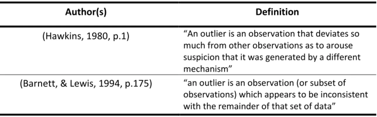
13 algorithm. For a start the two classical definitions of outlier are given in Table 2 - Classical outlier definitions.

Author(s)

Definition

(Hawkins, 1980, p.1)

much from other observations as to arouse suspicion that it was generated by a different mechanism”

(Barnett, & Lewis, 1994, p.175)

Table 2 - Classical outlier definitions

In this section techniques to detect outliers are presented. In general these techniques can be divided according to different features. In this work two of these features are described. The first feature identifies methods with underlying assumptions like, for example, that the data was generated by a certain type of distribution. These methods are called parametric. Their counterparts, the non-parametric methods, do not assume a specific type of underlying distribution.

The second feature by with outlier detection methods can be distinguished is by how many variables are considered when detecting an outlier. Univariate methods only consider the value of a single variable, while multivariate methods consider multiple dimensions to identify an outlier (Ben-gal, 2005).

The first method that is presented is called the percentile method. Using this method, all observations are ordered according to the dimension that should be scanned for outliers. Then a value above which points are considered outliers, and a value below which points are considered outliers are defined. Depending on the variable it can be appropriate to set zero as the lower limit. Usually both values are defined using percentiles of the dimension of interest. If an observation is spotted as an outlier its value can simply be set to the respective boundary. This method does not assume a specific kind of distribution, and thus is considered non-parametric.

The main advantage of this method is its low computational cost.

Disadvantages of this method are that the threshold above (or below) which an observation is an outlier must be determined manually. Also this is a univariate technique, and so only considers one dimension at a time. Another drawback is, that outliers are only determined by their rank of a specific variable, comparing with the rank of other observations. This method rigorously determines a chosen percentage of a sample as outliers, without caring about their localization comparing with the rest of the set.

14 procedure the number of outliers is not provided manually, but identified by the characteristic of the data.

A drawback is that this method assumes the variable to be normal distributed, which in reality is not always the case (Acuna & Rodriguez, 2004). This property makes it part of the parametric approaches.

Bay and Schwabacher (2003) proposed the so called simple distance based outlier detection. This method aims to identify the predefined number of outliers in a specific subset of the population. The procedure computes the average distance for all observations in the subset to their nearest neighbors. The size of the neighborhood, and the size of the subset are parameters of the algorithm. The neighborhood of an example can be chosen from the whole population. The observations with the highest average distance (the metric is also a parameter of the algorithm) to their nearest neighbors are considered outliers.

Bay & Schwabacher (2003) note that they do not provide any guideline for the right choice of the parameters, which also includes the size of the investigated subset. Desirable properties of this method are that it is a multivariate technique that does not make any assumption about the underlying distribution. On the other side it only identifies a pre-defined number of outliers, which might be difficult to guess.

The last presented method for detecting outliers is the local outlier factor (LOF). This method, proposed by Breunig, Kriegel, Ng, & Sander (2000) uses the concept of neighborhood. An integer k defines the number of neighbors. All observations at the same distance from the respective observation as the furthest neighbor are also called neighbors of this observation. As an effect of this the number of neighbors can vary if there are multiple neighbors at the same distance. The distance of the furthest neighbor is called k-distance. In the next step the so called reachability-distance is calculated. The reachability-distance between two objects is their distance, according to a metric, but at least the k-distance. So all neighbors are assumed to be at the k-distance. Note that this definition does not qualify to be a metric, because it is not symmetric. The distance from A to B can be different than the distance from B to A, if B is a neighbor of A, but not vice versa. This property is important when calculating the density of an observation. The so called local reachability density of a point is calculated as the inverse average reachability-distance from all its neighbors to the point.

The local outlier factor is defined as the average ratio of the local reachability densities of the neighbors and the point of interest. A value around one signifies that the investigated observation is approximately as dense as its neighbors, while a value that is much greater than one indicates that the investigated observation is a lot less dense than its neighbors. The latter is an indicator for an outlier.

In contrast to other methods, the proposed procedure does not strictly tell if an observations is an outlier, it rather assigns a degree of being an outlier to each observation, based on which the researcher can decide.

15 detection of different distributions within the same data set. While doing so it does not make specific assumptions about the underlying distribution, and thus is part of the non-parametric methods. Also the masking-effect2 _{can be tuned with the size of the neighborhood. If a greater neighborhood is} used, outliers are less likely to mask each other.

3.3.4.

Initializations for K-Means

As discussed above (Advantages and Disadvantages of K-Means) the k-means algorithm converges towards a local optimum, and the relation between initialization and result is deterministic. Therefore the initial centroids (seeds) have a major impact on the solution that will be found. This section will give an overview of different initialization techniques, which can be used in order to explore the search space in the most effective way possible.

The initialization methods are grouped by their relation of time performance to the data set’s complexity. Complexity is synonymous with the number of observations in the data set. At first the initialization techniques that show a linear relation of complexity and performance are presented. A (asymptotical) linear relation between complexity of the data set and the performance of the initialization means, that if the (already high) complexity of the data set increases by a certain proportion, the time it takes to perform the seed initialization increases by a similar proportion. This is, when the highest order of the time-complexity-relation is one.

- Forgy (1965) proposes a method, that assigns all observations to one of the k clusters at random, and then calculates the mean of each cluster. These means are used as initial seeds. - The method proposed by Jancey (1966) is to randomly generate seeds. Celebi, Kingravi, &

Vela (2013) note that, if the space is not filled with observations, this procedure might lead to empty clusters, when the generated values are too far apart from the data points.

- MacQueen (1967) suggested two methods of initialization. The first one assumes the first k observations to be the initial cluster centers, which has the drawback of being sensitive to the sorting of the data set. To overcome this disadvantage, the second method selects k randomly chosen observations to be the initial solutions. (Celebi et al., 2013) point out, that this allocates a higher probability for the initial cluster centers to be in an area of dense population, however there is no mechanism that prevents the chosen seeds to be outliers. - Ball & Hall (1967) take the overall centroid as a first seed, and the select arbitrary

observations, that have a minimal distance T to all previously chosen seed, until k seeds are defined. In many cases it is difficult to define a reasonable distance T, however it helps to provide a well spread initial solution. Tou and Gonzales (1974) use a similar method. The only difference is, that they use the first observation as the first seed, not the overall centroid.

2_{“It is said that an outlier masks a second one close by if the latter can be considered outlier by himself,}

but not any more if it is considered along with the first one. Equivalently after the deletion of one outlier other instance may emerge as an outlier. Masking occurs when a group of outlying points skews the mean and

16 - Gonzalez (1985) proposes an initialization method, which spreads out the cluster centers. It starts with one arbitrarily chosen observation, called the head of the cluster. Then one of the observations that is the furthest from this head is defined to be the head of the next cluster. Observations are assigned to one of the clusters based on which head is closest to them. Until the number of clusters is reached, the observation, that is the furthest from its head is defined to be the head of the next cluster, and all observations that are closer to the new head, than to their actual cluster heads, are assigned to the new cluster.

- Al-Daoud (1996) proposes a density based approach. In a first step the space is divided into M uniform hypercubes, which do not overlap. The total number of centroids is assigned to the hypercubes, proportionally to their respective number of observations. Each hypercube’s centroids are chose at random. Celebi et al. (2013) identify a disadvantage in the difficult choice of the number of hypercubes.

- Bradley & Fayyad (1998) also suggest a more stage procedure. At first the data set is partitioned into a number of randomly selected subsets. For each of those subsets k-means with the wanted number of clusters is applied. It should be initialized, using randomly chosen observations of the subset as seeds (second method proposed by (MacQueen, 1967), as described above). The resulting centroids from each subset are joined together into one superset. This set of centroids is then clustered by k-means a number of times. Each time, the centroids of another subset are chosen to be the seeds for the k-means algorithm in the superset. The seeds of the iteration with the smallest sum of square error are chosen to be the seeds for the k-means run on the whole population.

- Su & Dy (2007) suggest an initialization method that is using principal component analysis (PCA)3_{. The data set is divided according to a divisive algorithm. It uses the first principal} component of the covariance matrix that passes through the centroid of the data set. An orthogonal hyperplane is laid through the principal component, intersecting at the centroid. This plane divides the data set into two subsets. This procedure is repeated for the cluster with the greatest sum of square error, until the predefined number of clusters has been reached. The centroids of the resulting clusters serve as seeds for the k-means algorithm. - Another initialization method that uses principal component analysis is widely used. It

calculates the first two principal componenty, and initializes k equally distant seeds on the grid of the plane spanned by the first two principal components.

- Onoda, Sakai, & Yamada (2012) propose an initialization method based on Independent Component Analysis (ICA)4_{. An observations is chosen to be a seed if it has the minimum} cosine distance5 _{from one of the independent components.}

3_{Principal Component Analysis (PCA) is a technique that rotates the axis of a data set, so that a great}

proportion if the intrinsic information can be expressed with less dimensions. PCA projects the observations on the principal components of their covariance matrix. A principal component is an eigenvector multiplied with its eigenvalue. The principal components are ordered in descending order by the amount of variance they account for. In this algorithm, only the first principal component (accounting for the greatest proportion of variance) is considered. A discussion of Principal Component Analysis is not part of this work.

4_{Independent Component Analysis (ICA) is a technique that calculates new axis from the observations in}

17 At next initialization methods are presented, whose execution cost is loglinear to the complexity of the data set. Loglinear means, that the cost of execution is linear to a logarithm of the number of observations of the data set.

- Hartigan & Wong (1979) propose a method that first sorts all observations according to their distance from the overall centroid. This sorting procedure is the main cost driver for the initialization. Observations are chosen to be seeds by applying the formula (1 + (L – 1) * (M/K)) to their rank in the sorted data set. Where L is the number of the cluster (between 1 and the number of clusters), M is the total number of observations in the data set, and K is the total number of clusters. (Hartigan & Wong, 1979) point out that this initialization method guarantees, that none of the initial clusters will be empty.

- Al-Daoud (2005) presents a procedure that only takes one dimension in to consideration when initializing the seeds. This dimension is said to be the one with the greatest variance. All observations are ordered according to their values in that dimension, and then divided into k groups. The means of each group are chosen to be the initial centroids for the k-means algorithm.

- Redmond & Heneghan (2007) suggest a method that uses the kd-tree6 _{procedure. The} threshold to create leaf buckets is set to the number of observations divided by ten times the number of clusters wanted, so that each cluster has approximately ten buckets. For each leaf bucket, its density is computed as the division of number of observations by its volume. The volume can be simply obtained by multiplication of the length of all dimensions, where the length is the difference between the respective minimum and the respective maximum of a dimension in the leaf bucket. The density is then associated with the mean of the leaf bucket. The means are the potential seeds of the k-means algorithm, but only k should be chosen. Seeds should have two properties. They should represent a densely populated leaf bucket, and they should be well spread in the space. In order to optimize both constraints Redmond & Heneghan (2007) compute the distance between the leaf bucket means as the Euclidian distances weighted by their density. The first seed is the mean of the most dense leaf bucket. The second seed is chosen by the above described distance in descending order. The third and all subsequent seeds, until k is reached, are chosen using the distance to the closest seed (that has already been chosen), weighted by the density of the leaf bucket they represent.

independent of each other, they should still be correlated with the original data, in order to provide maximum interpretability.

5_{The cosine distance is a distance measure for two vectors. It is defined as the cosine of the angle}

between two vectors. If the observations of the two vectors are given the cosine distance can be computed as

where and are observations of the vectors A and B.

6_{A kd-tree (k-dimensional-tree) is a top-down hierarchical scheme of partitioning data. It splits a data}

18 Two problems are noted by Redmond & Heneghan (2007). First, the density for less dense leaf buckets is underestimated. So the distance computation is dominated by leaf buckets with a higher density. This drawback can be overcome by using the inverted rank density, instead of the absolute amount. (It needs to be inverted, so that the highest density is represented by the highest rank).

The second identified problem is, that outliers have impact on the density and the distance of a leaf bucket. In general outliers are an issue for k-means (Advantages and Disadvantages of K-Means). According to Redmond & Heneghan (2007) the effect of outliers on the distance causes the algorithm to choose observations from leaf buckets containing outliers as seeds, and the effect of the outliers on the mean of the leaf bucket would bias the true seed. They overcome this issue by assuming that outliers are mainly found in less dense leaf buckets. So they only consider 80% of the densest leaf bucket means to be potential seeds.

- Hasan, Chaoji, Salem, & Zaki (2009) propose a method that aims to avoid choosing outliers for seeding. They define six criteria that should be satisfied by their initialization method:

1. It should be computationally inexpensive

2. It should be parameter free, and if it uses parameters, they should not have a major influence on the seeds

3. It should be deterministic and not sensitive to the order of the data set

4. It should be not sensitive to outliers

5. It should be robust to clusters of different scale and density 6. It should be robust to different cluster sizes and skewness

19 The last part of this chapter presents initialization methods whose performance quadratically decreases with increasing complexity of the data set. Comparing with the other initialization methods, the ones that are presented here have a worse performance when the size of the data set increases.

- Lance (1967) proposes the usage of hierarchical algorithms to choose the location of seeds for k-means and leave the choice of similarity measure and metric to the user, because the right choice depends on the properties of the data set. The performance is determined by the performance of the applied hierarchical clustering algorithm. As stated in section Advantages and Disadvantages of K-Means, these algorithms generally take a large amount of time to process complex data sets. So the major drawback of this method is that it takes away k-mean’s advantage over hierarchical approaches, the fast execution.

- Astrahan (1970) defines his method based on two distance parameters. The first distance parameter defines the radius of an observation, which includes all its neighbors. The density of an observation is defined as the number of neighbors within that radius. All observations are sorted descendingly by their density. The densest observation is chosen to be the first potential seed. All remaining observations are defined as potential seeds in descending order of density, if they have at least at distance equal to the second parameter from their closest potential seed. This procedure is repeated until no further potential seed can be found. In case the number of potential seeds exceeds the number of wanted clusters, a hierarchical clustering algorithm is performed on all potential seeds. This hierarchical clustering algorithm is performed until the exact number of wanted seeds is reflected by the number of groups created by the algorithm. The centers of the resulting groups serve as initial seeds for k-means. Celebi et al. (2013) note that the major drawback of this method are the two distance parameters that have major influence on the resulting seeds and the standard implementation does not provide a heuristic for an educated guess to set them.

- Kaufman, & Rousseeuw (1990) define another method with a quadratic time-complexity relation. The algorithm choses the population mean as the first seed, and then the observation that reduces the sum of square error the most for each iteration. At each iteration the distances with the potentially new cluster seed have to be computed. This makes the procedure having a not desirable performance.

- Cao, Liang, & Jiang (2009) create a method that uses cohesion7 _{and coupling}8_{. These two} concepts serve different objectives. Cohesion is used as an indicator of centrally of an observation in its neighborhood, while coupling indicates the distance between two neighborhoods. Both concepts depend on the neighborhood of an observation. In order to define an appropriate neighborhood Cao et al. (2009) normalize all variables into a range

7_{The cohesion of an observation is defied by Cao et al. (2009) as the number of observations who’s}

neighborhood is a sub set of the neighborhood of the investigated observation. The number of observations for whom that applies is divided by the number of observations that share at least one element of their neighborhood with the neighborhood of the observation of interest. The higher the cohesion of an observation is, the more centrally it is located in its neighborhood.

20 between zero and one and compute the average distance between all observations (where the metric is subject to the researcher). They define this average distance as the neighborhood radius. All observations within that radius of an observation are called neighbors of the observation. Based on these neighbors, cohesion and coupling are calculated. The first cluster center is the observation with the maximal cohesion. All following initial centers are chosen in descending order by their cohesion. The second criteria they must satisfy is a coupling with all previously selected seeds, which is lower than the average distance between all observations. This procedure is stopped when the wanted number of seeds is reached.

3.3.5.

Number of Clusters

As mentioned above (Advantages and Disadvantages of K-Means), one of the major drawbacks of the k-means algorithm against hierarchical approaches is that the number of clusters needs to be pre-defined in k-means. This chapter provides some heuristics that help to choose a reasonable number of clusters.

As a first guideline Pham, Dimov, & Nguyen (2005) state that the number of clusters should be large enough to reflect the characteristics of the data set, but at the same time significantly smaller than the number of observations. The choice of the best number of clusters is similar to the question of whether the result of clustering is good or not. Therefore some of the techniques described in Internal Validation Techniques can be applied to determine reasonable k, as well. Oftentimes the number of clusters is defined by the business case, or by knowledge of the data source. All other cases need to use a heuristics. This chapter explains procedures that are customized for the purpose of evaluating the best number of clusters.

The first technique that is presented is X-Means. This method provides the applicant with the freedom of supplying a range of possible k, instead of a fix value. The idea of Pelleg & Moore (2000) is that a regular k-means algorithm is run with the lower boundary of the number of clusters. When the algorithm converges all final centroids (parents) are split into two children centroids and are moved apart from each other (proportional to the size of their cluster). In the next step local k-means are run within each cluster, using the two generated centroids as seeds. When this run has finished clusters are evaluated locally using the BID index (see: BIC-Index). If the solution with only the parent centroid scores a higher BIC-value than the children, it is kept. Otherwise the children are preferred over their parents. Then a new iteration of k-means is run on the whole population. This time it uses the suggested number of seeds from the previous run. This procedure stops when either the upper boundary of clusters has been reached, of the BIC-score does not improve anymore when adding new seeds.

Ray & Turi (1999) propose another procedure that uses a validity measure. This validity measure is computed as the ratio of the intra-cluster distance to the inter-cluster distance. Low values of this measure indicate good solutions, because both, a low intra-cluster distance and a high inter-cluster distance are desirable properties of a good clustering solution.

21 All observed values for the validity measure are compered, and the iteration that gave the lowest score determines the number of clusters.

Note that the validity measure can also serve as an indicator to choose better solutions over worse, when both options have the same number of clusters.

The cubic clustering criterion (CCC) is another technique of determining the number of clusters of a data set. It was proposed by Sarle (1983). It is based on the idea that good clustering solutions are able to explain a greater proportion of the overall variance, than a classifier that assumes that the data is equally distributed in the space. It is calculated using the formula:

is the expected value of under the assumption that the data is distributed equally in space It is obtained by the of hypercubes in which the space is divided. The number of hypercubes corresponds to the number of clusters to be checked for validity. In the formula denotes the actually observed by the obtained clusters, and K is a factor stabilize the variance Sarle (1983). K will not be further explained in this work since the main outcome of the CCC is determined by the previous term. Greater values of the cubic clustering criterion indicate a better grouping, because the centroids of the clusters seem to be more descriptive for the population.

However it should be noted that naturally raises with increasing number of clusters, and, therefore the cubic clustering criterion cannot be interpreted on its own. It is necessary to evaluate the context by computing the CCC for different numbers of clusters. The CCC will increase with the number of clusters, but the effect of an additional cluster will asymptotically decrease. It is subject to the specific problem to determine a rational number of clusters, which can be supported by the CCC.

3.4.

C

&

S

M

After different clustering algorithms have been introduced, and a number of initialization methods and distance measures have been explained. Now the clustering can be performed. Typically, in stochastic techniques, for each clustering problem many iterations are necessary until a satisfying solution has been found. This section gives conclusion about how a good solution can be distinguished from a bad solution.

As stated above (Definition), clustering seeks to identify groups in data where observations are similar insight the group, and different when compared across groups. This raises the question of how similarity should be measured. Although researchers have proposed a number of different similarity measures, a single best method cannot be defined. “Evaluating the quality of clustering results is still a challenge in recent research.” (Färber et al., 2010, p.1). In general the clusters should have a high intra-cluster similarity (low intra-cluster distances) and low inter-cluster similarity (high cluster distances). So one can say, the lower the intra-cluster-distance, the higher the inter-cluster-distance, the better is the validity of the segmentation.

The choice of a similarity measure/metric depends on the research question and the underlying type of data.

22 it shows a low intra-cluster standard deviation and a high inter-cluster standard deviation. This concept is picked up by some of the techniques below.

The two main branches of cluster validation are internal and external validation (Rendón, Abundez, Arizmendi, & Quiroz, 2011). Internal validation is based on information intrinsic to the data, while external information considers previous knowledge about the data (for example the true classification or distribution where observations were generated from).

The following sections will give an overview of popular cluster validation techniques.

3.4.1.

External Validation Techniques

For the external validation four indexes will be introduced. These indexes are the F-measure, entropy, purity, and the NMI-Measure. According to Rendón et al. (2011) these are the most frequently referenced in literature.

Following Powers (2011) the F-measure is based on two measures, Recall and Precision. In order to explain these measures, it is necessary to describe the concept of true positive, false positive, true negative, and false negative observations. These concepts are based on whether an observation is an event, or a non-event, and whether it was classified as an event, or a non-event. An event can be understood as the observation fulfilling some sort of criteria, like for example: Client owns a red car is an event in contrast to client does not own a red car would be a non-event. The following table translates the event/non-events to true/false positive/negative:

Event Non-Event

Classified as Event True Positive (TP) False Positive (FP) Classified as Non Event False Negative (FN) True Negative (TN) Table 3 - Translation from Event/Non-Event to True/False Positive/Negative. Correctly classified are

marked in green, while incorrectly classified observations are marked in orange.

The words “true” and “false” indicate whether an observation has been classified correctly, while the words “positive” and “negative” indicate whether an observation was classifies as an event or a non-event.

Having introduced these concepts, recall and precision will be defined consequently:

Recall is the True Positive Rate, which indicates the proportion of TP over all events. It gives conclusion about what fraction of all events have been classified as events.

23 Powers (2011) notes that neither of the measures captures information about how well the model handles negative cases. If information about negative cases should be gained, Inverse Recall and Inverse Precision can be calculated. These follow the same formulas as Precision and Recall, but exchange events with non-events. (For example: Client does not own a red car would be the event, while client owns a red car would be a non-event).

A classification is considered “good” when both measures are close to one. This is the case when there is only a minimal proportion of wrongly classified observations (orange fields in Table 3 - Translation from Event/Non-Event to True/False Positive/Negative. Correctly classified are marked in green, while incorrectly classified observations are marked in orange.). The F-measure is an attempt to combine Recall and Precision to a single indicator. Larsen & Aone (1999) calculate the F-measure as:

The F-measure increases when Precision or Recall increase and has a maximum of one, which is reached when both, Precision and Recall are equal to one. Therefore a higher F-measeure indicates a better fit of the model.

At next the concept of purity will be introduced. As the names says, it measures how pure a cluster is. The cluster purity is obtained, by taking the most frequent class of each cluster and divide it by the cluster size. So the cluster purity is the fraction of the most frequent class of a cluster. The overall purity is calculated by the weighted average of all cluster purities. The cluster purities are weighted by the respective cluster size divided by the total number of observations.

A model is considered “good” if it is very pure (if the model reflects the labels). In general great values (close to one) indicate good solutions. Nevertheless Strehl & Ghosh (2002) note, that purity is biased and favors smaller clusters. Clusters that only consists of one observation are scored as perfectly pure. They might be perfectly pure, but a model that defines every observation in a single cluster does not provide the needed information.

A measure that is similar to purity is entropy. In clustering entropy is defined as:

Originally Shannon (1948) introduced this measure without the index j. Here it is used to clarify that Entropy is calculated for each cluster.

In each cluster the negative sum of proportions of each class i is needed to define the entropy. It evaluates to zero if a cluster only consists of objects of the same class, and is greater when a cluster is less pure.

24 Strehl, Ghosh, & Mooney (2000) note that entropy should be preferred over purity, because it considers information about the whole distribution, and not only about the most frequent class. A different approach is the NMI-measure. NMI stands for normalized mutual information. The motivation for this measure is that oftentimes validity indexes depend on the chosen metric, and therefore lacking the opportunity to compare results from algorithms with different metric. Strehl et al. (2000) define the mutual information as:

Where K is the true labeling and is the result from the algorithm. Suppose that k denotes the number of true clusters, and g is the number of clusters that resulted from the algorithm. Consequently k * g is the number of possible combinations of k and g. Further, n denotes the total number of observations in the data set, and stands for the number of observations that were assigned to cluster h of the algorithm and have l as a true label. The sum stands for the number of observations that were assigned to cluster h by the algorithm, and the sum

signifies the number of observations that are truly labeled as l. Note that the base of the logarithm is not a parameter of the measure, because it does not have any effect on the result (it is reduced by the second algorithm of the same base). The term in the numerator of the log describes the ratio of observations that are in a specific combination of clusters (real label l and cluster h) over the expected number of observations under the assumption of independence. If this ratio is greater than one, it means, that more observations than expected are clustered as l and h. One signifies a match with the expected value, and a value between zero and one stands for a lower occurrence than expected. In a final step the weighted average over the log to the base k * g of these values is calculated. It is weighted by the fraction of observations with the respective combination of clusters. For the evaluation of the NMI-measure it can be said, that a higher value indicates a better fit for the actual labeling. It is worth noting that a positive property of the NMI-measure is, that, it punishes solutions that use many clusters, by dividing by the log of number of possible combinations of clusters.

3.4.2.

Internal Validation Techniques

Internal validation techniques distinguish from the external validation techniques in the need of information. By contrast, internal validation techniques do not require prior knowledge about the data, like for example a label, which indicates the true cluster of an observation (Larsen & Aone, 1999).

For the internal validation five indexes will be introduced in the following section these are the BIC, CH, DB, SIL, Dunn and NIVA indexes. It will be started with the BIC-index.