MULTI-PERIOD MEAN-VARIANCE PORTFOLIO OPTIMIZATION WITH
MARKOV SWITCHING PARAMETERS
Oswaldo L. V. Costa
∗ [email protected]Michael V. Araujo
∗ [email protected]∗Departamento de Engenharia de Telecomunicações e Controle
Escola Politécnica da Universidade de São Paulo CEP: 05508-900, São Paulo, SP, Brasil
ABSTRACT
In this paper we deal with a multi-period mean-variance port-folio selection problem with the market parameters subject to Markov random regime switching. We analytically derive an optimal control policy for this mean-variance formulation in a closed form. Such a policy is obtained from a set of in-terconnected Riccati difference equations. Additionally, an explicit expression for the efficient frontier corresponding to this control law is identified and numerical examples are pre-sented.
KEYWORDS: optimal control, Markov chain, stochastic sys-tems, portfolio optimization, multi-period mean-variance.
RESUMO
Investiga-se um modelo multi-dimensional de seleção de car-teiras em média-variância, no qual os parâmetros de mer-cado estão sujeitos a saltos Markovianos. Deriva-se ana-liticamente uma estratégia de controle ótima em forma fe-chada para esta formulação de média-variância. Esta estraté-gia é obtida através de um conjunto de equações a diferenças de Riccati. Adicionalmente, uma expressão explícita para a fronteira eficiente correspondente a este controle ótimo é identificada e exemplos numéricos são apresentados.
Artigo submetido em 24/05/2007 1a. Revisão em 04/06/2007 2a. Revisão em 12/03/2008
Aceito sob recomendação do Editor Associado Prof. José Roberto Castilho Piqueira
PALAVRAS-CHAVE: controle ótimo, cadeia de Markov,
sis-temas estocásticos, otimização de portfólio, média-variância em multi-período.
1
INTRODUCTION
In (Li and Ng, 2000) the market uncertainties are repro-duced by stochastic models in which the key parameters, expected return and volatility, are deterministic. As stated by (Zhang, 2000), such models are good only for a short period since they would not respond appropriately to ran-dom changes in these parameters due to some sudden mar-ket discontinuities (for example, the one caused by a terrorist strike). As a result, there has been an increasing interest in the study of financial models in which the key parameters are modulated by a Markov chain, see for instance (Bauerle and Rieder, 2004), (Yin and Zhou, 2004), (Zhang, 2000), (Zhou and Yin, 2003) and (Çakmak and Özekici, 2006). Indeed, such models can better reflect the market environment as the overall assets usually move according to a major trend given by the state of the underlying economy or by the general mood of the investors.
In (Çakmak and Özekici, 2006) and in (Yin and Zhou, 2004), discrete-time models for the mean-variance portfolio selec-tion problem with Markov switching were considered. It is important to stress the main differences between our work and these works. The basic idea in (Yin and Zhou, 2004) is to use the optimal strategy of the limit continuous time problem obtained in (Zhou and Yin, 2003) to derive a nearly optimal portfolio for the discrete time model presented in equation (6) of (Yin and Zhou, 2004). In (Çakmak and Özekici, 2006), the authors adopt a more direct approach to tackle the problem, avoiding any kind of approximating as-sumption as required in (Yin and Zhou, 2004), and obtain-ing optimal results, instead of nearly optimal as in (Yin and Zhou, 2004). However, all assets in the financial market con-sidered in (Çakmak and Özekici, 2006), including the risk free one, depend on a Markov chain. In our paper we follow a direct approach as in (Çakmak and Özekici, 2006), extend-ing their work in two other directions. First we consider a financial model more general than that in (Çakmak and Öze-kici, 2006), in which all assets are risky and dependent of a Markov chain. After that we consider a financial model in which there is a riskless asset independent of any source of uncertainty, even the Markov chain, and the risky ones, which depend on a Markov chain. In this case more spe-cific and interesting results can be analytically derived for the mean-variance portfolio selection problem with regime switching.
This paper is organized as follows. In Section 2 we formulate the model and the problems to be investigated. In Section 3, an optimal control policy for an auxiliary problem as well as the expected value and variance of the terminal wealth are analytically derived. Such a policy can be obtained by the so-lution of a set of interconnected Riccati difference equations. The solution of the mean-variance problems and an explicit expression for the efficient frontier are derived in Section 4. The case in which there is a riskless asset is considered in
Section 5. Numerical examples are presented in Section 6. The paper is concluded in Section 7 with some final remarks.
2
PROBLEM FORMULATION
Throughout the paper we shall denote by Rn the n-dimensional Euclidean real space and by Rn×m the Eu-clidean space of alln×m real matrices. For a sequence of numbersa1, . . . , am, we shall denote bydiag(ai)the
di-agonal matrix inRm×mformed by the elementa
iin theith
diagonal,i = 1, . . . , m. The superscript′ will denote the transpose of a vector or matrix. We will consider a finan-cial market withn+ 1risky securities on a complete filtered probability space(Ω,F,{Ft},P). The assets’ price will be described by the random vectorS¯(t) = (S0(t), . . . ,Sn(t))′ taking values in Rn+1 with t = 0, . . . , T. Set R¯(t) = (R0(t), . . . ,Rn(t))′, withRi(t) = Si(t+1)
Si(t) . We assume that the random vectorR¯(t)satisfies the following equation:
¯
R(t) = [¯e+ ¯µ(t, θ(t))] + ¯σ(t, θ(t))W(t), (1)
where ¯e = (1, e)′, with e ∈ Rn a vector with 1′s in all its components. Here {θ(t) ;t= 0, . . . , T} is a finite-state discrete-time Markov chain with state space
M = {1, . . . , m}, and {W(t); t = 0, . . . , T} is a sequence of (n+ 1)-dimensional independent random vectors with zero mean and covariance I (identity ma-trix). We assume that {W(t), θ(t)} are mutually in-dependent. The set M represents the possible opera-tions mode of the market. P is a probability mea-sure such that P(θ(t+ 1) =j|θ(0), . . . , θ(t) =i) =
P(θ(t+ 1) =j|θ(t) =i) = pij(t), pij(t) ≥ 0 and
P
j∈Mpij(t) = 1, for t = 0, . . . , T −1 and i, j ∈ M.
We set fort = 0, . . . , T, P(t) = [pij(t)]m×m, πi(t) = P(θ(t) =i), π(t) = (π1(t), . . . , πm(t))′. As in (Costa
et al., 2005), forz = (z1, . . . , zm)′ ∈ Rm, we define the
operatorE(z, t) = (E1(z, t), . . . ,Em(z, t))as Ei(z, t) =
m
P
j=1
pij(t)zj, fori∈ M. For notational simplicity, we shall
omit from now on the variabletinpij(t)andEi(z, t). The
filtrationFt is such that the random vectors {S¯(k) ;k = 0, . . . , t} and Markov chain {θ(k) ;k= 0, . . . , t} are Ft -measurable.
When the market operation mode is θ(t) = i ∈ M, ¯
µ(t, i) ∈ Rn+1 represents the vector with the ex-pected returns of the assets, while σ¯(t, i) ¯σ(t, i)′ ∈
R(n+1)×(n+1) is the covariance matrix of the returns. It will be convenient to decompose µ¯(t, i) and σ¯(t, i) as
¯
µ(t, i) =
µ0(t, i)
µ(t, i)
and ¯σ(t, i) =
σ0(t, i)
σ(t, i)
, with
µ(t, i) = (µ1(t, i), . . . , µn(t, i))′ ∈ Rn, σ0(t, i) =
(σ00(t, i), . . . , σ0n(t, i)) ∈ R1×n+1, and σ(t, i) =
E R¯(t) ¯R(t)′|θ(t) =i > 0, for eacht = 0, . . . , T −1 andi∈ M.
The set of admissible investment strategies U = {u = (u(0), . . . , u(T−1))} is such that for each i = 0, . . . , n and t = 0, . . . , T −1, u(t) = (u1(t), . . . , un(t))′, is
aFt-measurable random vector taking values inRn. We have thatu(t)represents the amount of the wealth allocated among thensecurities. Associated to each admissible in-vestment strategy u we have the portfolio’s value process
{Vu(t) ;t= 0, . . . , T −1}, which represents the investor’s
wealth at the end of timet. For notational simplicity, we shall suppress the superscriptuwhenever no confusion may arise.
Assuming that the initial wealthV (0) =V0>0and that the
portfolio is self-financed, the wealth process is represented by (see, for instance, (Li and Ng, 2000)):
V (t+ 1) =V (t) [1 +µ0(t, θ(t)) +σ0(t, θ(t))W(t)]
+u(t)′[µ(t, θ(t))−eµ0(t, θ(t))
+ (σ(t, θ(t))−eσ0(t, θ(t)))W(t)]. (2)
Note that the amount of wealth allocated to the asseti= 0 is determined byV(t)−e′u(t). DefiningA¯
θ(t)(t) = 1 +
µ0(t, θ(t)),Aeθ(t)(t) = σ0(t, θ(t)),B¯θ(t)(t) = µ(t, θ(t))−
eµ0(t, θ(t)), andBeθ(t)(t) =σ(t, θ(t))−eσ0(t, θ(t)), we can
rewrite (2) as:
V(t+ 1) =Aθ(t)(t)V(t) +Bθ(t)(t)′u(t), (3)
where
Aθ(t)(t) = ¯Aθ(t)(t) +Aeθ(t)(t)W(t)
and
Bθ(t)(t) = ¯Bθ(t)(t) +Beθ(t)(t)W(t).
The multi-period mean-variance problem aims at selecting u∈ U which has the greatest expected terminal wealth given an affordable terminal wealth variance, or which produces the lesser variance of the final wealth given a desirable ex-pected terminal wealth. Formally these problems, named re-spectivelyP1 σ2andP2 (ǫ), can be posed as:
P1 σ2: min
u∈U −E(V (T))
subject to :V ar(V (T))≤σ2 (4) P2 (ǫ) : min
u∈UV ar(V (T))
subject to :E(V(T))≥ǫ (5)
Alternatively, an unconstrained form would be:
P3 (ν) : min
u∈UνV ar(V (T))−E(V(T)), (6) where ν ∈ [0,∞) represents the investor’s risk aversion coefficient, giving his trade-off preference between the ex-pected terminal wealth and the associated risk level. Due
to the difficulty in solving directly the three problems above we shall consider, as in (Li and Ng, 2000), an auxiliary for-mulation. Using the fact thatνV ar(V (T))−E(V(T)) = νEV (T)2−νE2(V (T)) +E(V(T)), we can
asso-ciate toP3 (ν)the following auxiliary problem:
A(λ, ν) : min
u∈U E
n
νV (T)2−λV (T)o. (7)
3
OPTIMAL CONTROL POLICY FOR THE
AUXILIARY PROBLEM
In this section we obtain an explicit expression for the value function and optimal control policy for the auxiliary problem A(λ, ν)by applying dynamic programming. We also ob-tain closed expressions for the expected value and variance of the terminal wealth. As in the classical stochastic linear quadratic problem, this optimal control law depends on the solution of a set of recursive coupled Riccati difference equa-tions (see (8) below). Before going to the main result, let us define some intermediate problems. The value function for the auxiliary problem at timek ∈ {0, . . . , T−1}is defined by:
J(V (k), θ(k), k) = min
uk∈Uk
EnνV (T)2−λV (T)Fko,
where Uk = {uk = (u(k), . . . , u(T−1))′;u(t) is Ft
measurable for eacht = k, . . . , T −1}.We shall need the following definitions. For eachi∈ Mandt= 0, . . . , T, set:
χi(t) =E(Bi(t)) = ¯Bi(t),
φi(t) =E Bi(t)Bi(t)′
= ¯Bi(t) ¯Bi(t)′+Bei(t)Bei(t)′,
δi(t) =E
Ai(t)2
= ¯Ai(t)2+
eAi(t)
2
,
ϕi(t)′=E Ai(t)Bi(t)′
= ¯Ai(t) ¯Bi(t)′+Aei(t)Bei(t)′,
βi(t) =χi(t)
′ φi(t)
−1
χi(t),
Qi(t) =δi(t)−ϕi(t)′φi(t)−1ϕi(t),
Q(t) =diag(Qi(t)),
Ri(t) = ¯Ai(t)−χi(t)′φi(t)−1ϕi(t),
R(t) =diag(Ri(t)).
Notice that from the hypothesis that
E R¯(t) ¯R(t)′|θ(t) =i > 0, the inverse of φi(t) is
well defined and Qi(t) > 0. We compute backwards
the m dimensional vectors K(t) = (K1(t), . . . ,
Km(t))′, Z(t) = (Z1(t), . . . , Zm(t))′ and
D(t) = (D1(t), . . . , Dm(t))′, with Ki(t), Zi(t) and
Di(t)as follows: Fort=T−1, . . . ,0andi∈M:
Ki(t) =Qi(t)Ei[K(t+ 1)], Ki(T) =ν,
Zi(t) =Ri(t)Ei[Z(t+ 1)], Zi(T) =−λ,
Di(t) = E
i[Z(t+1)]2
From (8) we have by backward iteration that
K(t) = (Q(t)P(t)·. . .·Q(T−1)P(T−1))eν =νK(t),
and
Z(t) =−(R(t)P(t)·. . .·R(T−1)P(T−1))eλ =−λZ(t),
whereK(T) =νe, andZ(T) =−λe, and fort= 0, . . . , T,
K(t)∈RmandZ(t)∈Rmare defined as follows:
K(t) =
TY−1
k=t
Q(t)P(t)
!
e, Z(t) =
TY−1
k=t
R(t)P(t)
!
e.
(9) Equations (8) and (9) are related to the solution of problem (7) as stated in the next theorem.
We have the following theorem.
Theorem 1 The optimal control law for problem (7) is given by
u(t) = −φθ(t)(t)
−1
ϕθ(t)(t)V(t)
− Eθ(t)[Z(t+ 1)]
2Eθ(t)[K(t+ 1)]φθ(t)(t) −1
χθ(t)(t).(10)
Furthermore, the value function for the intermediate problem is
J(V(t), θ(t), t) = Kθ(t)(t)V (t)2+Zθ(t)(t)V(t)
+Dθ(t)(t). (11)
Proof: Let us apply induction ont. Fort=T we have that
J(V (T), θ(T), T) =νV (T)2−λV (T)
=Kθ(T)(T)V (T)2+Zθ(T)(T)V (T) +Dθ(T)(T),
in agreement with Theorem 1. Suppose the result holds for t = k+ 1. We show next that the solution also holds for t=k. Forθ(k) =i∈ MandV (k) =vwe have from the Bellman’s principle of optimality that
J(v, i, k) = min
u(k)E{J(V (k+ 1), θ(k+ 1), k+ 1)| Fk}
= min
u(k)E
n
Kθ(k+1)(k+ 1)V (k+ 1)2
+Zθ(k+1)(k+ 1)V(k+ 1)
+Dθ(k+1)(k+ 1)
Fk
= min
u(k){Ei[K(k+ 1)]
δ(k, i)v2
+2ϕ(k, i)′u(k)v+u(k)′φ(k, i)u(k)
+Ei[Z(k+ 1)]A¯(k, i)v+χ(k, i)′u(k)
+Ei[D(k+ 1)]}. (12)
Taking the derivative of (12) overu(k)and making the result equal to zero yields
2Ei[K(k+ 1)] [ϕ(k, i)v+φ(k, i)u(k)]
+Ei[Z(k+ 1)]χ(k, i) = 0 (13)
and from (13) we get (10). Substituting (10) into (12) yields the value function expressed in (11), providing the desired
result. ✷
Next we analytically derive expressions for the expected value and variance of the terminal wealth under the optimal control law (10). These expressions will be written in terms of some key parametersa,b,candd. First we make the fol-lowing definitions, related to the calculation of the expected value and variance of the portfolio, and used in the proof of Theorem 2. For eachj∈ Mandt= 0, . . . , T, define
hj(t) =
1 2
m
X
i=1
pijπi(t)
Ei[Z(t+ 1)]
Ei[K(t+ 1)]βi(t),
e
h(t) = (h1(t), . . . , hm(t))′, (14)
rj(t) =
1 4
m
X
i=1
pijπi(t)
Ei[Z(t+ 1)]
Ei[K(t+ 1)]
2
βi(t),
e
r(t) = (r1(t), . . . , rm(t))′, (15)
a=V(0)π(0)′Z(0), b=
TX−1
k=0
e
h(k)′Z(k+ 1),
(16)
c=V(0)2π(0)′K(0), d=
TX−1
k=0
e
r(k)′K(k+ 1).
(17)
Notice that from (14) and (15), 2er(k)′K(k + 1) =
eh(k)′Z(k+ 1)and thus from (16) and (17),2d= b. The constantarepresents the expected amount the investor ob-tains by investing in the reference assetj = 0and similarly bmultiplied by the ratio λ
ν yields the expected amount the
investor gets by investing in the assetsj 6= 0. The case in whichb= 0represents the situation in which it is not worth investing in these assets, as seen in the next theorem.
Theorem 2 Under the optimal control law (10), the ex-pected value and variance of the terminal wealth are:
E(V (T)) =a+λ
νb, (18)
V ar(V (T)) =c−a2−
λ ν
· b
2
4a−
λ ν
(1−2b)
.
(19)
Proof: First we proceed to find the expression for the ex-pected value of the final wealth. Using the control law (10) into (3), we get
V(t+ 1) =Aθ(t)(t)−Bθ(t)(t)′φθ(t)(t)−1ϕθ(t)(t)
·V (t)− Eθ(t)[Z(t+ 1)]
2Eθ(t)[K(t+ 1)]Bθ(t)(t) ′
φθ(t)(t)−1χθ(t)(t).
(20)
Letqj(t) = E V(t) 1{θ(t)=j}. From (Costa et al., 2005) and (20) it follows that
qj(t+ 1) = m
X
i=1
pijRi(t)qi(t)
−1
2
m
X
i=1
pijπi(t)
Ei[Z(t+ 1)]
Ei[K(t+ 1)]βi(t). (21)
Definingqe(t) = (q1(t), . . . , qm(t))
′
and replacing (14) into (21) leads to
e
q(t+ 1)′=qe(t)′R(t)P(t) +λ νeh(t)
′ ,
and thus
e
q(T)′ =qe(0)′
TY−1
k=0
R(k)P(k)
+λ ν
TX−1
k=0
e
h(k)′
TY−1
l=k+1
R(l)P(l).
Noting that E(V (T)) = Pmj=1EV (T) 1{θ(T)=j} =
e
q(T)′e, we have from (9) that
E(V(T)) =eq(0)′Z(0) +λ ν
TX−1
k=0
e
h(k)′Z(k+ 1). (22)
Substitutingaandb from (16) into (22), we get (18). Now we proceed to derive the expression for the variance of the final wealth as in (19). Taking square on both sides of (20) yields
V(t+ 1)2=Aθ(t)(t)2−2Aθ(t)(t)Bθ(t)(t)′φθ(t)(t)−1
·ϕθ(t)(t) +ϕθ(t)(t)′φθ(t)(t)−1
·Bθ(t)(t)Bθ(t)(t)
′
φθ(t)(t)
−1
ϕθ(t)(t)
V (t)2
−hAθ(t)(t)−Bθ(t)(t)
′
φθ(t)(t)
−1
ϕθ(t)(t)
· Eθ(t)[Z(t+ 1)]
Eθ(t)[K(t+ 1)]Bθ(t)(t) ′
φθ(t)(t)
−1
χθ(t)(t)
·V(t) +1 4
Eθ(t)[Z(t+ 1)]
Eθ(t)[K(t+ 1)]
2
χθ(t)(t)
′
·φθ(t)(t)−1Bθ(t)(t)Bθ(t)(t)′φθ(t)(t)−1 ·χθ(t)(t). (23)
Letgj(t) =E
V (t)21{θ(t)=j}
. From (Costa et al., 2005) and (23) it follows that
gj(t+ 1) = m
X
i=1
pijQi(t)gi(t)
+1 4
m
X
i=1
pijπi(t)
Ei[Z(t+ 1)]
Ei[K(t+ 1)]
2
βi(t).
(24)
Definingeg(t) = (g1(t), . . . , gm(t))′and from (15) we can
rewrite (24) as
e
g(t+ 1)′=eg(t)′Q(t)P(t) +
λ
ν
2
e
r(t)′
and thus
e
g(T)′ =eg(0)′
TY−1
k=0
Q(k)P(k)
+
λ ν
2TX−1
k=0
e
r(k)′
TY−1
l=k+1
Q(l)P(l).
Recalling thatEV(T)2=eg(T)′e, we have from (9) that
EV (T)2=eg(0)′K(0) +
λ
ν
2TX−1
k=0
e
r(k)′K(k+ 1).
(25) Replacingcanddfrom (17) into (25) and recalling thatd=
b
2, we obtain the expected square value of the final wealth as
EV(T)2=c+ λ ν
2 b 2.
Hence, from (18), we get that
V ar(V (T)) =EV (T)2−E(V(T))2
=c−a2−
λ ν b 2
4a−
λ ν
(1−2b)
,
which is the desired equation (19) for the variance of the final
wealth. ✷
4
SOLUTION OF THE PROBLEMS
We solve in this section the three mean-variance problems posed in Section 2 and explicitly derive an expression for the efficient frontier. LetΠ P1 σ2,Π (P2 (ǫ)),Π (P3 (ν))
andΠ (A(λ, ν))denote, respectively, the set of optimal so-lutions for problemsP1 σ2,P2 (ǫ),P3 (ν)andA(λ, ν).
We recall the following results, proved in (Li and Ng, 2000).
Proposition 2 Suppose that ν ≥ 0 andu ∈ Π (P3 (ν)). a) If V ar(Vu(T)) = σ2 then u ∈ Π P1 σ2. b) If
E(Vu(T)) =ǫthenu∈Π (P2 (ǫ)).
Next we present the solution of problemsP3 (ν),P1 σ2
andP2 (ǫ).
Theorem 3 An optimal strategy u for problems P3 (ν),
P1 σ2andP2 (ǫ)is given by (10) withK
i(t)andZi(t)
as in (8) andλ= 1+2νa
1−2b . For problemsP1 σ
2andP2 (ǫ),
νis given by
ν =
q b
2a2−2(1−2b)(c−σ2) for problemP1 σ2
b
ǫ(1−2b)−a for problemP2 (ǫ)
.
The expected value and variance of the terminal wealth are, respectively, given by
E(V(T)) = aν+b
ν(1−2b), (26)
V ar(V(T)) =c− a 2
(1−2b)+ b
2ν2(1−2b). (27)
Finally the efficient frontier of the multi-period mean-variance problem with regime switching is given by:
V ar(V(T)) =
c− a
2
(1−2b)
+(1−2b) 2b
E(V (T))− a
(1−2b)
2
.
(28)
Proof: From Proposition 1 if u ∈ Π (A(λ, ν))is such that λ = 1 + 2νE(Vu(T)) thenu ∈ Π (P3 (ν)). Combining
(18) and Proposition 1, we have
λ= 1 + 2νE(Vu(T))
= 1 + 2ν
a+λ νb
=⇒λ=1 + 2νa
1−2b . (29) Substituting (29) into (18) leads to (26). Replacing (29) into (19), we have (27). For problem P1 σ2 we have from
Proposition 2 and (27) that
σ2=V ar(Vu(T)) =c− a2
(1−2b)+ b 2ν2(1−2b),
and thusν =q b
2a2−2(1−2b)(c−σ2). For problemP2 (ǫ)we
have from Proposition 2 and (26) that
ǫ=E(Vu(T)) = aν+b ν(1−2b), and thusν= b
ǫ(1−2b)−a. Finally by combining (26) and (27)
and eliminating the parameterν, we have (28), completing
the proof. ✷
Notice that the efficient frontier equation has an hyperbolic shape with center0, a
(1−2b)
. The minimum variance of the
terminal wealth is given byV ar(V (T))min = c− a2 (1−2b)
and the expected terminal wealth associated to this portfolio isE(V(T))min= a
(1−2b).
Remark 1 Comparing Theorems 1 and 2, in which the fi-nancial market consists only of risky assets, with equations (20) and (34) to (38) in (Çakmak and Özekici, 2006), we can see that the hypothesis of the existence of a riskless asset depending on the Markov chain, as in (Çakmak and Öze-kici, 2006), produces no simplification on the final expres-sions for the control law and for the expected value and vari-ance of the final wealth.
5
THE SPECIAL CASE WITH ONE
RISK-LESS ASSET
Let us investigate now the special case in which one of the assets is riskless, that is, it has no volatility and it is unaf-fected by the Markov chain. We assume the asseti = 0as the riskless one. The price of the risk-free asset evolves as in (1), withσ0(t, i) = 0andµ0(t, i) = rf(t)for alltand
i∈M. The existence of a riskless asset allows us to simplify some equations in our model. Indeed, for eachi ∈ Mand t= 0, . . . , T, it follows that
¯
Ai(t) = ¯A(t) = 1 +rf(t),
δi(t) =E
Ai(t)2
= ¯A(t)2,
ϕi(t)′ =E Ai(t)Bi(t)′
= ¯A(t)E Bi(t)′
= ¯A(t)χi(t)′,
Ri(t) = ¯A(t) (1−βi(t))
and
Qi(t) = ¯A(t)Ri(t) = ¯A(t)2(1−βi(t)).
Set
ρ(t) =
TY−1
k=t
¯ A(k),
e
β(t) =diag(βi(t)),
and
e
Z(t) =
"TY−1
k=t
(I−βe(k))P(k)
#
e.
We have that
K(t) =ρ(t)Z(t),
e
h(t)′= 1
2ρ(t+ 1)π(t)
Z(t) =ρ(t)Ze(t), and
a=ρ(0)V (0)π(0)′Ze(0), c= (ρ(0)V(0))2π(0)′Ze(0), so thata2
c =π(0)
′ e
Z(0). We have the following result.
Theorem 4 An optimal strategy u for problems P3 (ν),
P1 σ2andP2 (ǫ)is given by
u(t) =−φθ(t)(t)−1χθ(t)(t)
¯
A(t)V(t)− λ
2νρ(t+ 1)
(30)
with λ and ν as in Theorem 3. Moreover, for this opti-mal control law, we have thatE(V (T))satisfies (26) and
V ar(V (T)) = b
2ν2(1−2b). The efficient frontier equation is
given by
V ar(V (T)) = (1−2b) 2b
E(V(T))− a
(1−2b)
2
. (31)
Proof: Suppose thatc = a2/(1−2b). Then the result is a
straightforward consequence of Theorem 3 observing that in (10),
Ei[Z(t+ 1)]
Ei[K(t+ 1)] =− λ νρ(t+ 1).
Remains to show thatc = a2/(1−2b). In order to show
that we show by induction onℓ= 0, . . . , T that
π(0)′Ze(0)+
ℓ−1
X
t=0
π(t)′βe(t)P(t)Ze(t+1) =π(ℓ)′Ze(ℓ). (32)
Clearly (32) holds forℓ = 0. Suppose it holds forℓ. Then recalling thatZe(ℓ) = [(I −βe(ℓ))P(ℓ)]Ze(ℓ+ 1), we have from (32) that
π(0)′Ze(0) +
ℓ
X
t=0
π(t)′βe(t)P(t)Ze(t+ 1)
=π(ℓ)′Ze(ℓ) +π(ℓ)′βe(ℓ)P(ℓ)Ze(ℓ+ 1)
=π(ℓ)′P(ℓ)−βe(ℓ)P(ℓ) +βe(ℓ)P(ℓ)Ze(ℓ+ 1)
=π(ℓ+ 1)′Ze(ℓ+ 1)
sinceπ(ℓ)′P(ℓ) = π(ℓ+ 1)′, showing (32). Noting that
e
Z(T) =eso thatπ(T)′Ze(T) = 1, it follows from (32) that
2b=
TX−1
t=0
π(t)′βe(t)P(t)Ze(t+ 1)
= 1−π(0)′Ze(0)
= 1−a 2
c ,
completing the proof. ✷
As a consequence of the existence of a risk-free asset, the minimum variance of the final wealth is zero with corre-sponding expected value of the terminal wealth given by E(V(T))min= a
(1−2b).
Remark 2 It should be noticed that the results of Theorems 3 and 4 coincide with those in (Li and Ng, 2000) for the case in which there are no switching parameters. Moreover, it is worth pointing out the difference between the expressions for the control strategy and for the expected value and vari-ance of the final wealth we find here considering the case in which there exists a riskless asset free of any source of uncertainty, and those expressions derived in (Çakmak and Özekici, 2006), in which the risk free security depends on the Markov chain.
6
NUMERICAL EXAMPLES
In this section we compare the model proposed in this paper with the one presented in (Li and Ng, 2000). The first exam-ple is the case in which all assets are risky while the second one includes a risk-free asset.
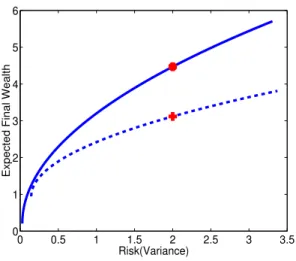
Example 1 Consider the case in which an investor with one unit wealth and an investment horizonT = 4has to allocate his possession among four risky assets in order to maximize his expected final wealthE(V(4)), while keeping the vari-ance of the terminal wealth not exceeding2, i.e.,σ2(4)≤2.
To simplify, we assume the multi-period process as station-ary. To determine the market trends we choose the S&P 500 Index (SPX) and, for the risky assets, we picked the four stocks which have more weight in this index: General Eletric (GE), Exxon Mobil (XOM), Citigroup (C) and Mi-crosoft (MSFT). The daily closing prices of these stocks, starting from 2000 until the end of 2004, are used to esti-mate the mean and variance of them. In this example, there are two major trends: up- or down-trend, i.e.,M= {1,2}, respectively. To identify which mode is leading the market we used a moving average. Whenever the monthly closing price of the index is above its three period moving aver-age, we define that month as an up-trend and whereas the monthly closing price of the index is bellow its three pe-riod moving average, we define the pepe-riod as a down-trend. To estimate the mean returnµ(t, θ(t))and covariance ma-trix σ2(t, θ(t))of the assets we follow an approach
0 0.5 1 1.5 2 2.5 3 3.5 0
1 2 3 4 5 6
Risk(Variance)
Expected Final Wealth
Figure 1: Efficient frontier
µ(t,2) = (−26.1%,−5.4%,−31.0%,−38.7%)′, and
σ2(t,1) =
8.9 1.7 5.6 3.9 1.7 5.2 2.2 1.3 5.6 2.2 9.0 4.0 3.9 1.3 4.0 12.7
/100,
σ2(t,2) =
14.1 3.9 9.5 8.0 3.9 7.4 3.9 3.7 9.5 3.9 15.7 8.2 8.0 3.7 8.2 19.6
/100.
As the number of up-trend days was almost 50% of the to-tal days, we choosepij = 0.5,i, j ∈ M, as the transition
probabilities. From (28), the mean-variance efficient frontier equation is given as follows:V ar(V(4)) = 0.029 + 0.108·
(E(V (4))−0.207)2. For the maximum selected risk level σ2(4) = 2, the corresponding expected final wealth in the efficient frontier isE(V (4)) = 4.47. We implemented the model proposed in (Li and Ng, 2000) to compare with the present one. To estimate the mean return and covariance ma-trix of the assets we use the whole period of the above sample (2000 - 2004) without separating the trend periods, obtaining fort = 0,1,2,3,µ(t) = (−4.2%,8.1%,7.6%,−14.2%)′ and
σ2(t) =
11.6% 2.9% 7.6% 6.1% 2.9% 6.3% 3.1% 2.5% 7.6% 3.1% 12.5% 6.2% 6.1% 2.5% 6.2% 16.4%
.
For this case, the mean-variance efficient frontier equation is given byV ar(V (4)) = 0.15 + 0.39·(E(V (4))−0.94)2. The expected terminal wealth corresponding to the selected risk level σ2(4) = 2isE(V (4)) = 3.12. In Fig. 1 we
can see the efficient frontier for both cases. The continuous line represent the efficient frontier for the case with regime
switching while the dotted line is the efficient frontier follow-ing the model proposed in (Li and Ng, 2000). The expected terminal wealth corresponding to the selected risk level is pointed out in Fig. 1 by an asterisk and by a cross, respec-tively for the case with and without Markov switching pa-rameters. Therefore, in this example, for the same accepted final risk level σ2(4) = 2,the first case delivered an
ex-pected final wealth above the case without jumps. This out-come illustrates the advantage of the present model to better capture the market movements.
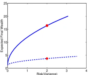
Example 2 Now we examine the situation with the
exis-tence of a riskless asset. In this example we use the same assets presented above plus a risk-free asset. The riskless asset is represented by the two years Fed Fund rate (GT2). Although this interest rate also changes following the mar-ket movements, we considered it constant and equal to its average in the period: rf(t) = 3.3%, for t = 0,1,2,3.
The objective is the same as above and we use the same assets and conditions as presented in the former example, just adding the riskless asset. We get the following mean-variance efficient frontier equation: V ar(V(4)) = 0.009·
(E(V(4))−1.14)2. Now, considering the model presented in (Li and Ng, 2000), with the same data as in the last ex-ample and adding the riskless asseti = 0we get the fol-lowing efficient frontier equation: V ar(V (4)) = 0.30·
(E(V(4))−1.14)2. The expected terminal wealth in each situation isE(V(4)) = 16.41andE(V (4)) = 3.72, re-spectively. These two points are plotted in Fig. 2 by an as-terisk and a cross, respectively for the case with and without regime switching. In Fig. 2, we plotted the two efficient fron-tier equations. As in the former example, the outcome of the case with the key parameters modulated by a Markov chain (solid line) beat by far the case without this feature (dotted line).
7
CONCLUSIONS
In this paper we extended the work of (Çakmak and Öze-kici, 2006) by studying a discrete-time multi-period mean-variance portfolio selection problem subject to Markovian jumps in the parameters. An optimal investment strategy for this mean-variance problem was analytically derived in a closed form. We showed that this optimal policy depends upon a set of interconnected Riccati difference equations pre-sented in (8). As a result, an explicit expression for the efficient frontier was identified. Our results coincide with those in (Li and Ng, 2000) for the case in which there are no switching parameters. The advantage of this model is to better respond to drastic movements of the market as a result of stress situations or discontinuity changes due to external factors.
for-0 1 2 3 4 0
5 10 15 20 25
Risk(Variance)
Expected Final Wealth
Figure 2: Efficient frontier with a riskless asset
mulation presented here could be obtained by considering a generalized multi-period mean variance portfolio optimiza-tion problem with Markov switching parameters, as studied in (Costa and Araujo, 2008). The generalized multi-period mean-variance problem can be seen as an stochastic con-trol problem in which the objective function is formed by a weighted sum of a linear combination of the expected value and square of the expected value of the wealth, and the ex-pected value of the square of the wealth. A great variety of mean-variance models with intermediate restrictions and/or intermediate costs in the objective function can be derived from this generalized formulation. The usefulness of adopt-ing this kind of criterion is that in several situations investor managers have to report their portfolio’s return in a periodic basis to their beneficiaries, clients or to governmental au-thorities, so that intermediate performances are as important as the final one. Moreover intermediate restrictions could also be included in this formulation (see also (Costa and Nabholz, 2007)). Therefore more traditional mean-variance problems, which regards the performance only at the final value, would not be the most appropriate for these situations. On the other hand the price one pays by adopting this more general approach is that a solution for the problem usually requires a numerical procedure based on a Lagrangian dual minimization problem (see (Zhu et al., 2004), (Costa and Araujo, 2008)).
ACKNOWLEDGMENT
The first author received financial support from CNPq (Brazilian National Research Council), grant 304866/03-2 and FAPESP (Research Council of the State of São Paulo), grant 03/06736-7. The authors would like to express their gratitude to the associate editor and referees for their
sugges-tions and helpful comments.
REFERENCES
Bauerle, N. and Rieder, U. (2004). Portfolio optimization with Markov–modulated stock prices and interest rates,
IEEE Trans. Autom. Control49: 442–447.
Çakmak, U. and Özekici, S. (2006). Portfolio optimization in stochastic markets,Math. Methods Oper. Research
63: 151–168.
Costa, O. L. V. and Araujo, M. V. (2008). A generalized multi-period mean-variance portfolio optimization with Markov switching parameters,Automatica, to appear.
Costa, O. L. V., Fragoso, M. D. and Marques, R. P. (2005).
Discrete–Time Markov Jump Linear Systems, Springer– Verlag.
Costa, O. L. V. and Nabholz, R. (2007). Multiperiod mean-variance optimization with intertemporal restric-tions,Journal of Optimization Theory and Applications
134: 257–274.
Li, D. and Ng, W. (2000). Optimal dynamic portfolio selec-tion: Multi-period mean–variance formulation, Math. Finance10: 387–406.
Markowitz, H. (1952). Portfolio selection,J. Finance7: 77– 91.
Yin, G. and Zhou, X. Y. (2004). Markowitz’s mean– variance portfolio selection with regime switching: From discrete–time models to their continuous–time limits,IEEE Trans. Autom. Control49: 349–360.
Zhang, Q. (2000). Stock trading: An optimal selling rule,
SIAM J. Control Optim.40: 64–87.
Zhou, X. Y. and Yin, G. (2003). Markowitz’s mean– variance portfolio selection with regime switching: A continuous–time model, SIAM J. Control Optim.
42: 1466–1482.