REM WORKING PAPER SERIES
On the Performance of US Fiscal Forecasts: Government vs.
Private Information
Zidong An, João Tovar Jalles
REM Working Paper 0130-2020
May 2020
REM – Research in Economics and Mathematics
Rua Miguel Lúpi 20, 1249-078 Lisboa,
Portugal
ISSN 2184-108X
Any opinions expressed are those of the authors and not those of REM. Short, up to two paragraphs can be cited provided that full credit is given to the authors.
REM – Research in Economics and Mathematics
Rua Miguel Lupi, 20 1249-078 LISBOA Portugal Telephone: +351 - 213 925 912 E-mail: [email protected] https://rem.rc.iseg.ulisboa.pt/ https://twitter.com/ResearchRem https://www.linkedin.com/company/researchrem/ https://www.facebook.com/researchrem/
On the Performance of US Fiscal Forecasts: Government vs.
Private Information
*Zidong An
João Tovar Jalles
#May, 2020
Abstract
This paper contributes to shed light on the quality and performance of US fiscal forecasts. The first part inspects the causes of official (CBO) fiscal forecasts revisions between 1984 and 2016 that are due to technical, economic or policy reasons. Both individual and cumulative means of forecast errors are relatively close to zero, particularly in the case of expenditures. CBO averages indicate net average downward revenue and expenditure revisions and net average upward deficit revisions. Focusing on the causes of the technical component, we uncover that its revisions are quite unpredictable which casts doubts on inferences about fiscal policy sustainability that rely on point estimates. Comparing official with private-sector (Consensus) forecasts, despite the informational advantages CBO might have, one cannot unequivocally say that one or the other is more accurate. Evidence also seems to suggest that CBO forecasts are consistently heavily biased towards optimism while this is less the case for Consensus forecasts. Not only is the extent of information rigidity is more prevalent in CBO forecasts, but evidence also seems to indicate that Consensus forecasts dominate CBO’s in terms of information content.
Keywords: forecasting performance, encompassing tests, CBO, Consensus JEL Classification: C53, E17, H62
* Acknowledgments: This work was supported by the FCT (Fundação para a Ciência e a Tecnologia) [grant numbers UID/ECO/00436/2019 and UID/SOC/04521/2019]. Authors thank Alan Auerbach for insightful discussions on the topic including to an earlier version of this paper. The usual disclaimer applies. The views expressed are those of the author(s) and do not necessarily represent those of the IMF, or its member countries.
International Monetary Fund, Research Department, 700 19th Street NW, Washington DC, 20431, USA. E-mail:
# ISEG – School of Economics and Management; REM – Research in Economics and Mathematics, UECE – Research
Unit on Complexity and Economics, University of Lisbon, Portugal. Centre for Globalization and Governance and Economics for Policy, Nova School of Business and Economics, New University of Lisbon, Portugal. Email:
2 1. Introduction
Over the recent years, a key issue in the design of fiscal policy has been the accuracy of government budget forecasts, both on the revenue and expenditure side. Since budgeting is about the future, budget decisions regarding the allocation of resources must be based on forecasts. However, according to Aaron (2000) “budget forecasts are always wrong, and often they are wrong by a lot”. Moreover, forecasts are unlikely to become significantly more accurate in the future not because they are compiled by unskilled technicians (who do their work conscientiously), but because inaccuracy is inherent to the unscientific state of the economic science. The persistence of overly optimistic forecasts led to the perception that, as budget forecasts came to occupy a more central role in the political process, the pressure on forecasters to help policy makers avoid hard choices led to forecasting bias.
The accountability of governments for the use of public funds in democracies is at the root of budgetary procedures and has led to the development of fiscal forecasting techniques. Such accountability requires a clear understanding of the impact of macroeconomic developments and discretionary government action on both government revenue and expenditure. Not surprisingly, therefore, fiscal forecasting and monitoring has always received attention from policy makers, monetary policy authorities, international economic organizations, financial market analysts, rating agencies, research institutions and the general public.
In the academic literature, there is a wealth of papers evaluating forecast records, more often for the macroeconomic side of the economy than for the fiscal side and even fewer taking a budgetary disaggregated approach. Given the role played by both revenue and expenditure forecasts in budgeting processes1, almost all national fiscal policy agencies have implemented some kind of forecasting procedure based on either judgment, simple regressions, time series methods, structural macro-econometric models, or some combination of different techniques.
1 An overwhelming majority of the existing papers dealing with short- and medium-term fiscal projections or
attempting to assess the effect of the cycle on the budget focus on government revenues, in particular on important items such as Wage Taxes, Sales Taxes or Value Added Taxes, and Social Contributions (Lawrence et al., 1998, and Van den Noord, 2000). However, it is not unusual to see short-term forecasting models of the spending side of the budget (Mandy (1989), Tridimas (1992), Pike and Savage (1998) and Giles and Hall (1998)).
3
Government targets have been criticized for being systematically biased as a result of setting unrealistic, politically motivated targets (Strauch et al., 2004; Moulin and Wierts, 2006).2 Governments' fiscal policies come under particular scrutiny and deviations of actual paths of key fiscal variables from those initially planned may spark a great deal of debate and criticism. The literature on forecast performance supports the view that fiscal forecasts prepared by governments tend to be biased3 and inaccurate4. More importantly, assessing the causes for forecast errors is relevant for monitoring purposes and allow for the continuous improvement of forecasts by learning from past errors.5 Sizeable, systematic or biased forecast errors in certain items would presumably allow fiscal analysts to identify weaknesses in their forecasting procedures. Auerbach (1999) states that "one needs more data to get a better sense of whether the recent (budget) forecasts really are consistent with forecast efficiency, or whether they simply illustrate the continuation of a process of biased forecasting".
This paper revisits the issue of fiscal forecast performance using the US' Congressional Budget Office (henceforth, CBO) data over a long time span from 1984 until 2016. Secondly, we pay special attention to the causes of forecast errors by distinguishing them according to their source (economic, policy or technical) so as to get a better idea of the extent to which what are called "errors" are attributable to institutional forecasting conventions. Moreover, we look at both government revenue as well as government expenditure predictions separately. Finally, we compare official (CBO-based) fiscal forecasts to the ones emerging from the private sector (proxied by Consensus Economics). This last point is in line with the observation that the period of the "Great Moderation" between 1982 and 2007 has affected the time series properties of many variables and the fact that official forecasts have deteriorated considerably (relative to private sector ones) since the 1990s (D'Agostino and Whelan, 2008; Gamber and Smith, 2009).
2 A great deal of literature has analyzed the potential bias the political and institutional process might have on revenue
and spending forecasts (Plesko, 1988; Feenberg et al., 1989; Auerbach, 1995 and 1996; Bruck and Stephan, 2006), and the nature and properties of forecast errors within national states (Gentry, 1989; Baguestani and McNown, 1992; Campbell and Ghysels, 1995; Auerbach, 1999; Mühleisen et al., 2005).
3 Jonung and Larch (2006) claim that in some euro area countries biased forecasts (targets) by the governments have
played an important role in the generation of excessive deficits in the past.
4 For a recent cross-country study assessing the forecasting performance and accuracy of fiscal predictions using a
plethora of techniques, see Jalles et al. (2015).
5 Papers that have also looked at causes of forecast errors for different countries include the works by Beetsma et al.,
4
Our results show that between 1984 and 2016, both individual and cumulative means of forecast errors are relatively close to zero, particularly expenditures. Moreover, the CBO averages indicate net average downward revenue and expenditure revisions and net average upward deficit revisions, with cumulative values over the six-year revision period averaging about -1.3 and -0.3 percent of GDP for revenue and expenditure, respectively. If policy components are excluded, we find evidence of hardly enormous errors. Focusing on the causes of the technical component, as a result of unexpected behavioral responses, we uncover that its revisions are quite unpredictable which, ultimately, make us suspicious of inferences about fiscal policy sustainability that rely on revenues’ and/or expenditures’ point estimates. We also find evidence of serial correlation for government revenues (less so for expenditures). We then compared official with private-sector (Consensus) forecasts, despite the informational advantages CBO might have, one cannot unequivocally say that one or the other is more accurate. CBO appears to be more accurate for current year predictions. However, Consensus is (weakly) preferred for year-ahead forecasts as far as accuracy is concerned. Moreover, evidence seems to suggest that CBO forecasts are consistently heavily biased towards optimism while this is less the case for Consensus forecasts. Not only is the extent of information rigidity is more prevalent in CBO forecasts, but evidence also seems to indicate that Consensus, by pooling many individual forecasts, dominate CBO forecasts in terms of information content.
The remainder of the paper is organized as follows. Section 2 discusses the data underlying the empirical section. Section 3 evaluates CBO's fiscal forecasts’ performance. In Section 4 we compare CBO forecasts with Consensus Economics’ ones. The last section concludes.
2. Data
The Congressional Budget Office produces twice each year (and, sometimes, more frequently) revenue and expenditure forecasts for the current and several upcoming fiscal years. One forecast typically occurs around the beginning of February with the presentation of the "Economic and Budget Outlook" by CBO. The second typically occurs in August or September, with CBO's
5
"Economic and Budget Outlook: an Update". For most of the sample period, both winter and summer forecasts have been for six fiscal years.6
The reasons to focus on CBO forecasts are twofold: firstly, the methodology underlying the CBO is probably the one that has been consistently more stable over the last decades when compared with the Office of Management and Budget projections alternative. Secondly, in between the two sources, the CBO projections are probably the ones which have been less distant from true forecasts since projections from the Office of Management and Budget were regularly distorted by budget rules (Reischauer, 1990).
According to Auerbach (1994) one can find three possible reasons behind the persistence of deficits in the US: high "baselines", unexpected behavioral responses and additional forecast errors. He distinguishes between three types of errors: policy errors, economic errors and technical
(behavioral) errors. Policy errors are due to errors on the course of fiscal policy, owing to the
implementation of new, not yet announced by the forecast cut-off date, fiscal policy measures or cancellation of the previously announced measures.7 Economic errors are those that can be explained by wrong forecasts of macroeconomic variables that are used in the budget projections. Finally, technical errors would be due to other ("residual") factors, for example, a shift in the composition of capital income from dividends to capital gains, or a change in the distribution of income, or a revision in revenue resulting from a change in the rate of tax evasion. They might in part stem from behavioral responses but also from model mis-specification. Factors such the impact of macroeconomic forecast errors and data revisions have not been extensively covered. Exceptions include the studies by Jong-A-Pin et al. (2012) and Beetsma et al. (2013).8 These factors are intertwined with the forecasting procedures by a given institution, the treatment of assumptions and other variables, the forecast horizon, the nature of data, and the level of detail and
6 Recently, CBO has begun to report forecasts over an eleven-year horizon.
7 Note that is should not be confused with “political” errors. In fact, any political economic dimension to forecast
revisions is outside the scope of this paper.
8 In addition, Eschenbach and Schuknecht (2004) and Morris and Schuknecht (2007) point to the impact of asset price
6
aggregation a forecaster might want to pursue. Next, we will attempt to address some of these issues.
3. A look into the causes of forecast errors: Evaluating CBO Forecasts
In addition to the historical examination of forecasting performance, a real-time forecaster needs to understand the causes of the errors. In revising its revenue and expenditure forecasts for a particular year, each government agency incorporates changes in its own economic forecasts as well as estimates of the effects of policy changes. For a number of years, CBO has followed the practice of dividing each forecast revision into three mutually exclusive categories: policy, economic, and technical. More formally, we may express this revision process as:
t h t h t h t h t h x p e r x , 1,1 , , , (1)
where xh,t is the h-step-ahead forecast at date t and
p
h,t,e
h,t andr
h,t are, respectively, the policy,economic, and technical components of the revision in this forecast from period t-1. Because there are two forecasts made each year for revenues and expenditures in each of six fiscal years, there are twelve forecast horizons and twelve corresponding revisions for the revenues and expenditures of each fiscal year being predicted.9 Odd-numbered revisions are those occurring between winter and summer; even-numbered revisions are those occurring between summer and winter. For example, the revision at horizon 7 included in, say, the 1998 Midsession Review was the change in the forecast revenue (expenditure) for fiscal year 2001 from that given one period earlier, in winter 1998.
3.1 Revision Patterns and Statistical Properties
Table 1 presents basic means for CBO forecast revisions for both revenues and expenditures, for the period 1993-2016. To ensure that revisions from different years comparable, each revision is scaled by nominal GDP and expressed in percentage terms. The mean cumulative revision is equal to the sum of the means at each forecast horizon; it represents an estimate of the cumulative
9 The last such revision, however, differs from the others, in that it reflects changes over the very brief period between
the late summer forecast during the fiscal year itself and the September 30 end of that fiscal year. Thus, similarly to Auerbach (1999), in our analysis below, we take only the first eleven forecast revisions for each fiscal year, labeling these revisions 1 (shortest horizon, from winter to summer during the fiscal year itself) through 11 (longest horizon, five years earlier).
7
revision (in percent of GDP) during the period from initial to final published forecast for a given fiscal year's revenue or expenditure.
Table 1. Average Forecast Revisions, by horizon, 1984-2016 (percent of GDP)
CBO Revenue CBO Expenditure CBO Deficit
Technical Economic Policy Total Technical Economic Policy Total Technical Economic Policy Total
Spec. 1 2 3 4 5 6 7 8 9 10 11 12 Horizon 1 0.01 0.04 -0.05 0.01 -0.18 0.00 0.08 -0.13 -0.19 -0.04 0.12 -0.14 2 -0.10 -0.09 -0.22 -0.40 -0.07 -0.04 0.08 -0.05 0.02 0.05 0.30 0.35 3 0.01 0.04 -0.04 0.01 0.03 -0.03 0.18 0.17 0.03 -0.07 0.22 0.16 4 -0.08 -0.13 -0.13 -0.34 0.03 -0.07 -0.03 -0.11 0.10 0.06 0.11 0.24 5 -0.01 0.00 -0.01 -0.02 0.04 -0.03 0.14 0.12 0.05 -0.03 0.15 0.14 6 -0.05 -0.16 -0.08 -0.28 0.04 -0.07 -0.07 -0.15 0.09 0.08 0.01 0.13 7 -0.01 0.00 0.01 0.00 0.05 -0.03 0.14 0.10 0.05 -0.03 0.13 0.11 8 -0.03 -0.15 -0.06 -0.23 0.06 -0.08 -0.11 -0.20 0.08 0.07 -0.05 0.03 9 -0.01 0.02 0.04 0.04 0.04 -0.03 0.16 0.12 0.05 -0.04 0.12 0.08 10 -0.03 -0.15 0.01 -0.17 0.02 -0.09 -0.14 -0.32 0.04 0.06 -0.15 -0.14 11 -0.01 0.04 0.06 0.08 0.04 -0.01 0.15 0.11 0.06 -0.05 0.09 0.03 Average -0.03 -0.05 -0.04 -0.12 0.01 -0.04 0.05 -0.03 0.04 0.01 0.10 0.09 Sum -0.30 -0.54 -0.48 -1.31 0.09 -0.48 0.58 -0.34 0.39 0.07 1.06 0.98
Source: authors’ computations.
A natural consequence of the theory of optimal forecasts is that these should have no systematic bias (assuming the perceived costs of forecast errors being symmetric). Over a long period, then, the average forecast errors should not differ significantly from zero. Looking at the averages in Table 1, then, the most notable aspect of these individual means is that they are relatively close to zero, particularly in the case of expenditures. Indeed, the CBO averages indicate net average downward revenue and expenditure revisions and net average upward deficit revisions, with cumulative values over the six-year revision period averaging about -1.3 and -0.3 percent of GDP for revenue and expenditure, respectively. For revenues, the highest fraction (in absolute value) comes from the economic component, while for expenditures the policy component explains most of the revision.
It is interesting to note that revenue revisions in odd horizons are generally of higher mean than the revisions at even horizons. In terms of timing, this translates the fact that optimism is more present in the summer than in the winter (but there is no obvious reason behind the existence of more pessimism in the winter, at the time of the initial budget presentation). The opposite applies to expenditures, where optimism is more present in the winter, perhaps more in line with a pre-conception that initial forecasts are given more attention and hence carrying greater political weight. Furthermore, whereas in the case of revenues (winter) as the forecast horizon shortens, the magnitude of revisions increases due to a much higher relative contribution from the policy
8
component, in the case of expenditures (summer) the opposite applies. This can be visualized by plotting both sets of revisions for revenues and expenditures in the two periods, summer and winter – Figure 1.
Figure 1. Revenues', Expenditures', and Deficits' Revision by Component in Summer and Winter Periods, 1984-2016
However, if one breaks the sample down into sub-periods (based on the sample's mid-point), as is done in Table 2, it is clear that the aggregate results mask very different experiences during the two distinct periods. The first decade of the 21st century is marked by both a higher downward revision in revenues and an upward revision in expenditures with the highest share attributed to policy components. The Global Financial Crisis affected the relationship and relative magnitude of each component. Policy chances became more relevant since this direct
9
governmental tool took renewed prominence in a continuous effort to react and respond to the negative effects of the negative shock. One example of such policy was the American Recovery and Reinvestment Act of 2009 (ARRA) which included, on the revenue side, both tax cuts and deductions. Such policy changes are at the heart of the increase in the relatively importance of this component when revising fiscal forecasts. Note also that revenues are typically more elastic than expenditures with respect to movements in GDP. Consequently, during bad times economic changes contribute to downward revisions in revenue forecasts. Output forecasts tend to be more optimistic during crisis periods and also tend to be rigid when incorporating new information. In fact, as shown in An, Jalles and Loungani (2018) economists do a very poor job in forecasting recessions correctly. These authors also show that strong booms are also missed, providing suggestive evidence for Nordhaus' view that behavioral factors—the reluctance to absorb either good or bad news—play a role in the evolution of forecasts. As output forecasts are revised downward, so are revenue forecasts in the same direction. 10
Table 2. Average Forecast Revisions, by horizon, 1984-2000 vs. 2001-2016 (percent of GDP)
Panel A. Forecast Periods: 1984-2000
CBO Revenue CBO Expenditure CBO Deficit
Technical Economic Policy Total Technical Economic Policy Total Technical Economic Policy Total
Spec. 1 2 3 4 5 6 7 8 9 10 11 12 Horizon 1 0.06 0.06 0.00 0.11 -0.17 -0.01 0.02 -0.17 -0.23 -0.07 0.02 -0.28 2 0.00 -0.09 0.06 -0.04 -0.08 -0.02 -0.05 -0.16 -0.07 0.06 -0.11 -0.12 3 0.05 0.09 0.04 0.17 0.04 -0.03 0.03 0.01 -0.02 -0.12 -0.01 -0.15 4 -0.01 -0.11 0.06 -0.07 0.03 -0.05 -0.07 -0.16 0.04 0.05 -0.12 -0.09 5 0.05 0.07 0.07 0.17 0.06 -0.04 -0.01 -0.04 0.01 -0.11 -0.08 -0.21 6 -0.01 -0.09 0.04 -0.07 0.06 -0.05 -0.10 -0.19 0.07 0.04 -0.13 -0.12 7 0.04 0.03 0.08 0.14 0.06 -0.04 -0.03 -0.10 0.01 -0.08 -0.11 -0.24 8 -0.01 -0.09 0.05 -0.06 0.10 -0.06 -0.13 -0.24 0.11 0.03 -0.19 -0.18 9 0.04 0.02 0.10 0.15 0.05 -0.04 -0.03 -0.11 0.02 -0.06 -0.13 -0.25 10 -0.01 -0.12 0.05 -0.09 0.02 -0.08 -0.17 -0.40 0.03 0.05 -0.22 -0.31 11 0.04 0.01 0.12 0.16 0.03 -0.04 -0.07 -0.21 -0.01 -0.05 -0.19 -0.37 Average 0.02 -0.02 0.06 0.05 0.02 -0.04 -0.05 -0.16 -0.01 -0.02 -0.12 -0.21 Sum 0.24 -0.22 0.68 0.58 0.19 -0.47 -0.60 -1.75 -0.05 -0.25 -1.26 -2.31
Panel B. Forecast Periods: 2001-2016
CBO Revenue CBO Expenditure CBO Deficit
Technical Economic Policy Total Technical Economic Policy Total Technical Economic Policy Total
Spec. 1 2 3 4 5 6 7 8 9 10 11 12 Horizon 1 -0.05 0.02 -0.11 -0.09 -0.19 0.00 0.13 -0.09 -0.14 -0.01 0.24 0.00 2 -0.19 -0.09 -0.49 -0.76 -0.07 -0.06 0.20 0.07 0.11 0.03 0.69 0.83 3 -0.05 -0.02 -0.14 -0.18 0.03 -0.02 0.37 0.35 0.08 0.00 0.51 0.52 4 -0.15 -0.16 -0.32 -0.63 0.02 -0.09 0.02 -0.05 0.17 0.07 0.34 0.58 5 -0.08 -0.09 -0.12 -0.25 0.02 -0.02 0.34 0.30 0.10 0.07 0.45 0.55 10 We thank an anonymous referee.
10 6 -0.09 -0.23 -0.21 -0.53 0.03 -0.10 -0.05 -0.11 0.12 0.13 0.17 0.42 7 -0.08 -0.06 -0.09 -0.19 0.03 -0.02 0.38 0.36 0.11 0.04 0.47 0.55 8 -0.05 -0.22 -0.19 -0.45 0.01 -0.09 -0.07 -0.16 0.05 0.12 0.12 0.29 9 -0.08 0.02 -0.04 -0.10 0.02 0.00 0.42 0.44 0.10 -0.02 0.46 0.54 10 -0.05 -0.18 -0.05 -0.28 0.01 -0.11 -0.11 -0.21 0.07 0.07 -0.07 0.07 11 -0.09 0.08 -0.04 -0.04 0.07 0.05 0.50 0.61 0.16 -0.03 0.53 0.65 Average -0.09 -0.08 -0.16 -0.32 0.00 -0.04 0.19 0.14 0.08 0.04 0.35 0.46 Sum -0.95 -0.92 -1.78 -3.52 -0.03 -0.46 2.12 1.49 0.92 0.46 3.90 5.01
Source: authors’ computations.
Note: “Technical”, “Economic” and “Policy” refer to technical, economic and policy components in associated forecast revisions. Refer to the main text for further details.
Plotting the winter/summer revisions similarly to Figure 1, one gets Figure 2 and 3. In the former we can see that the period 2001-2016 is associated with much higher revisions than the period 1984-2001. Whereas in the first sub-period the economic component had a relatively big importance, in the second sub-period the policy component becomes the largest contributor to the revisions (particularly in the winter). In the case of expenditures, Figure 3, the second sub-period is equally associated with higher revisions. In this case, the policy component was more important contributor in winter revisions in the 1984-2000 period and in summer revisions in the 2001-2016 period. Finally, the deficit revisions mimic more or less closely those from expenditures’ (Figure 4).
11
Figure 2. Revenues' Revisions by Component in Summer and Winter: 1984-2000 and 2001-2016
12
Figure 3. Expenditures' Revisions by Component in Summer and Winter: 1984-2000 and 2001-2016
13
Figure 4. Deficits' Revision by Component in Summer and Winter: 1984-2000 and 2001-2016
As mentioned in section 2, policy changes are due to laws enacted; economic changes result from revision the agency has made to its macroeconomic forecasts. Both are considered external factors that are determined prior to the finalization and presentation of budget forecasts. In contrast, only the technical changes arise from the budget forecasting process. The focus of this paper is on fiscal forecasts, hence we focus more strongly on technical changes which is the “error” component one does not control directly and should try to understand so as to minimize it. Given the relatively big role attributed to the technical component, the analysis below will pay special attention on technical forecast errors, for they might arise, partly, as a result of unexpected behavioral responses. CBO does build some behavioral responses into its forecasts; the controversy is about whether these predicted responses are large enough. Moreover, unlike economic forecast errors, technical forecast errors correspond to the residuals stemming out of the forecast process which are not directly related to aggregate adjustments. Understanding their causes seems as an important exercise. Furthermore, to the extent that deficits in more recent years have been caused by
14
inaccurate assessments, one could anticipate this to appear in technical forecast errors. In line with Auerbach (1995) we estimate the following equation:
it it t i i it
P
R
1
(2)where
R
it is the technical forecast error for i=r,e corresponding to government revenue, government expenditure respectively, and fiscal year t; and Pt1it is an estimate of the change inrevenues or expenditures in year t resulting from policy changes during year t-1. Thus, equation (2) assumes that behavior responds to the previous year's policy changes. Table 3a presents regression results for the case of government revenues. Recall that these policy variables give the estimated effect on the current fiscal year's revenue of earlier calendar year's legislation. Since calendar and fiscal years overlap, we include the policy variables from both the most recent calendar year and the one preceding it. Table 3b replicates for the case of government expenditures. The stochastic terms of the estimated equations also require further consideration. Each observation is a forecast error over the 20-month period beginning eight months before the fiscal year being evaluated. Hence, successive observations overlap for an eight-month period. Given this, one should expect successive error terms
it to be correlated, even if the underlying disturbances themselves were serially uncorrelated across fiscal years. Each observation's error should have an MA(1) structure:1
t t t
(3)where
t is the component of the disturbance arising during the fiscal year itself. The parameter15
Table 3.a Revenue Technical Forecast Revisions by horizon, 1984-2016
Horizon (1) (2) (3) (4) (5) (6) (7) (8) (9) (10) (11) Policy L1 1.2736** 0.3129*** -0.0073 0.1211 0.2174 0.1236* 0.1454 -0.2001 0.0727 -0.2038 0.0469 (0.5248) (0.0417) (0.1728) (0.0853) (0.1760) (0.0746) (0.1660) (0.1649) (0.1183) (0.1252) (0.0962) Policy L2 -0.6552 -0.0585 -0.0033 -0.1588*** 0.1202 -0.1665 0.1190 -0.0400 0.0976 -0.0250 0.0875 (0.9079) (0.0941) (0.2074) (0.0483) (0.1292) (0.1720) (0.0877) (0.0535) (0.0724) (0.0370) (0.0579) Cons 0.0350 -0.0431 -0.0137 -0.0909 -0.0038 -0.0462 -0.0156 -0.0236 -0.0271 -0.0247 -0.0291 (0.0642) (0.0711) (0.0721) (0.0748) (0.0496) (0.0507) (0.0462) (0.0489) (0.0466) (0.0392) (0.0465) MA(1) -0.0737 0.3350 0.3924 0.3167** 0.3180 0.0451 0.3089* 0.3205 0.3727* 0.4274* 0.3972* (0.4385) (0.2529) (0.2957) (0.1473) (0.1943) (0.2551) (0.1870) (0.2749) (0.2025) (0.2305) (0.2196) No. of Obs. 28 28 27 27 27 26 27 25 27 24 26 Pseudo R-sq 0.21 0.36 0.12 0.21 0.21 0.06 0.18 0.07 0.20 0.11 0.21
Source: authors’ estimates.
Note: OLS estimates of equations 2 and 3 – refer to the main text. Heteroskedastic-consistent robust standard errors are reported in parenthesis. *, **, *** indicate significance at 10%, 5% and 1% levels, respectively.
Table 3a provides a number of interesting results. First, the MA term, whenever statistically significant, is positive as one would expect. The once-lagged policy variable has a positive and statistically significant coefficient in 3 out of 11 regressions, as one would predict if behavioral effects were overstated (the twice-lagged variable is seldomly statistically significant). In the case of expenditures (Table 3b) the once-lagged policy variable has a positive and statistically significant coefficient in only 2 out of 11 regressions. The lack of statistical significance throughout may reflect the level of aggregation of both total revenues and expenditures. Another comment worth making involves the constant term, which represent the average overprediction of revenues (always negative even if not statistically significant) and underprediction of expenditures (generally positive) that remain unexplained. Sensitivity analysis of these results does not substantially alter our main findings (such as omitting the second-lagged policy variable).
Table 3.b Expenditure Technical Forecast Revisions by horizon, 1984-2016 Horizon (1) (2) (3) (4) (5) (6) (7) (8) (9) (10) (11) Policy L1 -0.0147 -0.5341 0.0896 0.0115 0.1376 -0.0446 0.1824** -0.0775 0.1361* -0.1377 0.0674 (0.6822) (0.3322) (0.1476) (0.0962) (0.0995) (0.0730) (0.0824) (0.0698) (0.0747) (0.0858) (0.0719) Policy L2 -0.9504 -0.0538 -0.0469 0.0620 -0.0876 0.0163 -0.0826 0.0428 -0.0780 -0.0026 -0.0126 (0.8034) (0.1844) (0.1079) (0.1615) (0.1240) (0.1451) (0.0970) (0.1508) (0.0883) (0.0896) (0.0580) Cons -0.1114* -0.0392 0.0335 0.0237 0.0465 0.0406 0.0394 0.0481 0.0385 -0.0076 0.0381 (0.0612) (0.0993) (0.0604) (0.0551) (0.0878) (0.0496) (0.0471) (0.0732) (0.0467) (0.0721) (0.0367) MA(1) 0.2224 -0.0573 0.1630 0.3798*** 0.1874*** 0.3008*** 0.1354 0.3459*** 0.2958* 1.0000*** 0.2694** (0.2472) (0.3118) (0.3528) (0.1391) (0.0539) (0.1102) (0.1041) (0.0920) (0.1738) (0.0000) (0.1365) No. of Obs. 28 28 27 27 27 26 27 25 27 24 26 Pseudo R-sq 0.14 0.16 0.03 0.14 0.05 0.14 0.11 0.21 0.18 0.29 0.13
Source: authors’ estimates.
Note: OLS estimates of equations 2 and28 – refer to the main text. Heteroskedastic-consistent robust standard errors are reported in parenthesis. *, **, *** indicate significance at 10%, 5% and 1% levels, respectively.
16
Can we explain technical errors? To answer this question, we begin by regressing each technical revision for each fiscal year on a constant term and on the lagged values of the three forecast revisions for the same fiscal year. Our results11 show that technical revisions are essentially unpredictable using this information - very low R-squares and no regressor yields an impact that is statistically different from zero at usual levels. Even incorporating a time trend to the econometric specification does not significantly increase its explanatory power. On the one hand it is improbable that such trend will keep up for long. On the other, conditional of having a better understanding on the underlying process, we should cast doubts on inferences about fiscal policy sustainability that rely on point estimates of revenues or expenditures.
One possible explanation for the observed pattern of government forecast revisions is that the aggregate forecasts considered do not really represent statistical predictions of future revenues or expenditures, but rather "baseline" projections that take into account assumptions about future policy that are inconsistent with optimal forecasting procedures. By practice, baseline forecasts of policy are in some cases determined by certain mechanical rules that do not reflect expectations regarding future policy. Hence, many of the revisions attributed to policy changes do not represent "surprises," but simply the application of these rules. Therefore, if one wishes to determine the extent to which forecasts reflect the unbiased and efficient use of available information, it is useful to exclude policy revisions from the analysis. One might further divide the remaining revisions into their "economic" and "technical" components, making it possible (potentially) to determine the extent to which forecasting errors arise from underlying macroeconomic forecasts, as opposed to other factors. This is a useful exercise: we now focus solely on these two components together, represented by the sum
e
h,t
r
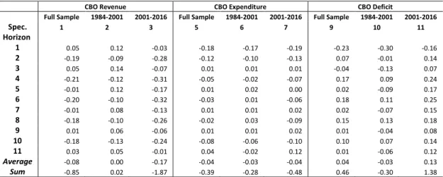
h,t in equation (1). Table 4 repeats the calculations of Tables 1 and 2, excluding revisions attributed to policy changes. In its first three sets of columns, the table presents estimates for the full sample period and well as the sub-periods considered before. We observe that in the case of revenue revisions the cumulative value has fallen by almost half to -0.85 percent of GDP, whereas the expenditure cumulative value has remained more or less
17
unchanged; that is, once policy components are removed, over the six-year revision period we find evidence of hardly enormous errors.
Table 4. Average Economic and Technical Forecast Revisions, by horizon (percent of GDP)
CBO Revenue CBO Expenditure CBO Deficit
Full Sample 1984-2001 2001-2016 Full Sample 1984-2001 2001-2016 Full Sample 1984-2001 2001-2016
Spec. 1 2 3 5 6 7 9 10 11 Horizon 1 0.05 0.12 -0.03 -0.18 -0.17 -0.19 -0.23 -0.30 -0.16 2 -0.19 -0.09 -0.28 -0.12 -0.10 -0.13 0.07 -0.01 0.14 3 0.05 0.14 -0.07 0.01 0.01 0.01 -0.04 -0.13 0.07 4 -0.21 -0.12 -0.31 -0.05 -0.02 -0.07 0.17 0.09 0.24 5 -0.01 0.12 -0.17 0.01 0.02 0.00 0.02 -0.09 0.17 6 -0.20 -0.10 -0.32 -0.03 0.01 -0.06 0.18 0.11 0.25 7 -0.01 0.08 -0.13 0.01 0.01 0.02 0.02 -0.07 0.15 8 -0.18 -0.10 -0.26 -0.02 0.03 -0.09 0.15 0.13 0.18 9 0.01 0.06 -0.06 0.01 0.01 0.02 0.01 -0.04 0.08 10 -0.18 -0.13 -0.24 -0.08 -0.06 -0.10 0.10 0.07 0.14 11 0.03 0.05 -0.01 0.04 -0.02 0.12 0.01 -0.06 0.12 Average -0.08 0.00 -0.17 -0.04 -0.03 -0.04 0.04 -0.03 0.13 Sum -0.85 0.02 -1.87 -0.39 -0.28 -0.48 0.46 -0.30 1.38
Source: authors’ computations.
3.2 Forecast Evaluation
Using the individual forecast revisions underlying the means in Table 1, one can construct formal tests of forecast efficiency. Consider the relationship between successive forecast revisions for the same fiscal year,
y
h,t andy
h t1 , 1. According to theory, if each forecast is unbiased anduses all information available at the time, these revisions should have a zero mean and should be uncorrelated. Letting
a
h be the mean forecast revision for horizon i, we relate these successive forecasts by the equation:t h h t h h t h t h h t h h h t h y y or a y a y , 1 , 1 , , 1 1 , 1 , ( ) (4)
where
h
a
h
ha
h1and
h,t has zero mean and is serially independent.12The hypothesis of forecast efficiency implies that
a
h
0
(no bias) and
h
0
(no serialcorrelation). The mean values,
a
h, in equation 4 have already been presented, in Table 1. Table 512 For revisions at horizon 11, there is no lagged revision, so equation (4) becomes
t t
t
a
18
presents estimates of the coefficients
h. At the bottom of each column of estimates we presentthe p-values corresponding to F-tests of two joint hypotheses related to forecast efficiency. The first is that all means are zero (
a
h
0
); the second, is that all correlation coefficients are zero (0
h
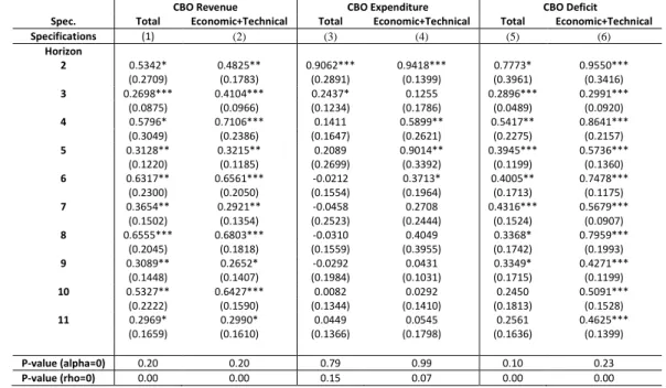
). The coefficients in the first two columns of the table - for government revenues -, show substantial serial correlation13; this is less true in the case of government expenditures (specifications 3 and 4). As discussed above, one might have expected some of this serial correlation to be due to the presence of the policy component in each forecast. However, it turns out that eliminating the policy components of the successive revisions actually strengthens the results, typically increasing the estimated serial correlation coefficients. For revenues (both total and economic+technical), all serial correlation coefficients are positive, and the hypothesis that all are zero is strongly rejected (last row). This suggests a partial adjustment mechanism, with not all new information immediately incorporated into forecasts. One can readily imagine institutional reasons for such inertia. For example, it might be perceived as costly to change a forecast and then rescind the change, leading to a tendency to be cautious in the incorporation of new information in forecasts. As far as expenditures are concerned, when economic+technical is considered we find stronger evidence rejecting the null of no serial correlation; (which was absent when total was considered in specification 3 - p-value in excess of 10 percent). Finally, throughout Table 5, the joint test on the
′s suggests the absence of bias (and yet again results are strengthened in the economic+technical case).
13 The finding of serial correlation in revenue forecasts is not a new one. For example, Campbell and Ghysels (1995)
19
Table 5. Serial Correlation of Successive Forecast Revisions, by horizon, 1984-2016
CBO Revenue CBO Expenditure CBO Deficit Spec. Total Economic+Technical Total Economic+Technical Total Economic+Technical Specifications (1) (2) (3) (4) (5) (6) Horizon 2 0.5342* 0.4825** 0.9062*** 0.9418*** 0.7773* 0.9550*** (0.2709) (0.1783) (0.2891) (0.1399) (0.3961) (0.3416) 3 0.2698*** 0.4104*** 0.2437* 0.1255 0.2896*** 0.2991*** (0.0875) (0.0966) (0.1234) (0.1786) (0.0489) (0.0920) 4 0.5796* 0.7106*** 0.1411 0.5899** 0.5417** 0.8641*** (0.3049) (0.2386) (0.1647) (0.2621) (0.2275) (0.2157) 5 0.3128** 0.3215** 0.2089 0.9014** 0.3945*** 0.5736*** (0.1220) (0.1185) (0.2699) (0.3392) (0.1199) (0.1360) 6 0.6317** 0.6561*** -0.0212 0.3713* 0.4005** 0.7478*** (0.2300) (0.2050) (0.1554) (0.1964) (0.1713) (0.1175) 7 0.3654** 0.2921** -0.0458 0.2708 0.4316*** 0.5679*** (0.1502) (0.1354) (0.2523) (0.2444) (0.1524) (0.0907) 8 0.6555*** 0.6803*** -0.0310 0.4049 0.3368* 0.7959*** (0.2045) (0.1818) (0.1559) (0.3955) (0.1742) (0.1993) 9 0.3089** 0.2652* -0.0292 0.0431 0.3349* 0.4271*** (0.1448) (0.1407) (0.1984) (0.1031) (0.1715) (0.1199) 10 0.5327** 0.6427*** 0.0082 0.0292 0.2450 0.5091*** (0.2222) (0.1590) (0.1344) (0.1410) (0.1813) (0.1528) 11 0.2969* 0.2990* 0.0449 0.0545 0.2561 0.4625*** (0.1659) (0.1610) (0.1366) (0.1798) (0.1636) (0.1399) P-value (alpha=0) 0.20 0.20 0.79 0.99 0.10 0.23 P-value (rho=0) 0.00 0.00 0.15 0.07 0.00 0.00
Source: authors’ estimates.
In what follows, we compare CBO-based aggregate deficit forecasts with those coming from the private sector, proxied by Consensus Economics' predictions for the budget balance-to-GDP ratio.
4. CBO vs. Private Sector
Some of the differences in forecast performance identified above appear large; others appear small. An interesting question is: which of these comparisons shows a really significant difference in performance, and which show differences which are not really significant given the small sample size and the volatility of the target variable? To some extent this is a subjective issue. For instance, it can be argued by a user in government that the differences between CBO and, say, Consensus Economics (private) forecasters in predicting business investment are not operationally important, since all the errors are large, and the variable is not in any case a key policy target. On the other hand, small differences in forecasts of policy-sensitive variables like the budget balance may be of great practical importance. Fiscal policy is a major government tool to direct the developments in the society and, more narrowly, in the economy. However, a user of macroeconomic forecasts in a multinational company might have a quite different perspective, and give a high weight to forecasts of, for instance, investment and industrial production. Because of
20
such problems in assigning weights to variables to reflect their relative importance, we do not attempt to pool forecast errors across different variables in this study. However, we do conduct two sets of tests for the statistical significance of differences in errors for the US budget balance-to-GDP ratio using both CBO and Consensus forecasts.
In this section, for comparison purposes vis-a-vis the CBO deficit forecasts, we resort to the Consensus Economics service. Earlier studies in the literature have also pointed out the deficiencies of government budget forecasts. See Leal et al. (2008, p. 350) for a discussion of previous studies, which include Strauch et al. (2004), Moulin and Wierts (2006), Annett (2006), Jonung and Larch (2006), and Pina and Venes (2011). Moreover, Frankel and Schreger (2014) find that private sector forecasts exhibit less bias than government forecasts. Hence, it is recommended that government forecasts should be supplemented by private sector forecasts, which are presumably less subject to the political pressures that governments face.14 Each month since 1989, the Consensus Economics has published forecasts for major economic variables prepared by panels of 10-30 private sector forecasters. Below the individual forecasts for each variable, the service publishes their arithmetic average, the "consensus forecast" for that variable. Consensus forecasts are known to be hard to beat (Batchelor and Dua, 1992). 15
This means that, in practice, the most promising alternative to official forecasts, such as the CBO, for most users of economic forecasts is not some naive model, but a consensus of private sector forecasts (Artis, 1996; Loungani, 2001). Since Consensus does not provide forecasts of neither government revenues nor government expenditures independently, we have to rely on the budget balance forecasts. In other words, we use the mean of the private analysts' monthly consensus forecasts of budget balance-to-GDP ratios for the current and next year between February 1993 and September 2016. From this point forward, the remainder of the analysis will
14 Carabotta and Clayes (2015) demonstrate that the accuracy of fiscal forecasts might be improved by combining the
forecasts of both private and public agencies. We thank an anonymous referee for this suggestion.
15 A detailed cross-country analysis of the performance and underlying characteristics of consensus fiscal forecasts is
21
be carried out over the period 1993-2016 (period during which both sources of forecasts – CBO and Consensus – overlap).
4.1 Forecast Accuracy and Test for Bias
The standard comparative measures used in the literature (such as the Mean Forecast Error, Mean Absolute Error and Root Mean Squared Error) are interesting when evaluating the unconditional forecast performance of a given institution (Keereman 1999; McNown, 1992; Artis and Marcellino, 2001; Pérez, 2007). We begin by presenting some summary statistics about the budget balance forecast error - i.e. the difference between the outcome and the forecast. Or equivalently:
𝐹𝐸𝑡,ℎ𝐶𝐵𝑂 = 𝐺𝐵𝐵𝑡− 𝐹𝑡,ℎ𝐶𝐵𝑂 (5a)
𝐹𝐸𝑡,ℎ𝐶𝐹 = 𝐺𝐵𝐵𝑡− 𝐹𝑡,ℎ𝐶𝐹 (5b)
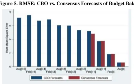
where 𝐹𝐸𝑡,ℎ is the budget balance forecast error for target year t with forecast horizon h, 𝐺𝐵𝐵𝑡 is the actual budget balance value, and 𝐹𝑡,ℎ is the budget balance forecast. We rely on the root mean square (forecast) error (RMSE). Figure 5 below shows that for those months for which we have both CBO and Consensus forecasts, the RMSE is very similar. Hence, one cannot unequivocally say that one or the other is more accurate.
Figure 5. RMSE: CBO vs. Consensus Forecasts of Budget Balance
22
Next, we perform a standard test to assess the existence of bias in forecasts. Following Holden and Peel (1990) specification, we have to run the following couple of regressions:
𝐹𝐸𝑡,ℎ𝐶𝐵𝑂 = 𝑎ℎ𝐶𝐵𝑂 + 𝜀𝑡,ℎ (6a)
𝐹𝐸𝑡,ℎ𝐶𝐹 = 𝑎ℎ𝐶𝐹+ 𝜇𝑡,ℎ (6b)
Under the null hypothesis that 𝑎ℎ = 0, then the underlying forecast is unbiased. If 𝑎ℎ < 0, then
the forecast is biased toward optimism; conversely, if 𝑎ℎ > 0, the forecast is biased toward pessimism. Figure 6 plots the results (the coefficient estimates for 𝑎ℎ) for different forecast horizons for both CBO and Consensus budget balance forecasts. Evidence seems to suggest that CBO forecasts are consistently heavily biased towards optimism while this is less the case for Consensus forecasts.
Figure 6. Test for Bias: CBO vs. Consensus Forecasts of Budget Balance
Source: authors’ estimates.
4.2. Forecast comparison: WEO vs Consensus
To test differences in forecast accuracy, we check the null hypothesis of no difference in the accuracy of two competing forecasts by employing the Diebold and Mariano’s (1995) (DM) test. The authors proposed to base the comparison on the following statistic:
𝐷𝑀ℎ = 𝑇−1/2 ∑
𝑑𝑡,ℎ 𝑇 𝑡=1
23
where 𝑑𝑡,ℎ = 𝑔(𝐹𝐸𝑡,ℎ𝐶𝐵𝑂) − 𝑔(𝐹𝐸𝑡,ℎ𝐶𝐹) is the loss function of interest. With quadratic loss, 𝑔(𝐹𝐸) = 𝐹𝐸2; with absolute loss, 𝑔(𝐹𝐸) = |𝐹𝐸|.16 Looking at Table 6, CBO appears to be more accurate for current year predictions. However, Concensus is (weakly) preferred for year-ahead forecasts as far as accuracy is concerned.
Table 6. Difference in Accuracy, by horizon
Specification (1) (2) (3) (4)
Year Ahead Current Year
Horizon Apr[t-1] Oct[t-1] Apr[t] Oct[t]
Absolute (MAE) 0.21 -0.01 -0.05* -0.04*
(0.15) (0.05) (0.03) (0.02)
More accurate CBO CBO
Quadratic (MSE) 1.74* 0.09 -0.04 -0.01
(0.98) (0.13) (0.05) (0.02)
More accurate Consensus
Note: standard errors in parenthesis. ***, **, * denote statistical significance at the 10, 5 and 1 percent level, respectively. Source: authors’ estimates.
Next, to test the significance of differences in bias, we use a test developed by Ashley et al. (1980). The test involves running a regression between the differences in errors from two competing methods (in our case, CBO and Consensus), and the sums of these errors. In mathematical terms, this means estimating the following regression:
∆𝑡,ℎ= 𝛽1+ 𝛽2∙ (𝛴𝑡,ℎ− 𝛴̅̅̅̅̅) + 𝜔𝑡,ℎ 𝑡,ℎ (8)
where ∆𝑡,ℎ= 𝐹𝐸𝑡,ℎ𝐶𝐵𝑂 − 𝐹𝐸𝑡,ℎ𝐶𝐹 and 𝛴𝑡,ℎ = 𝐹𝐸𝑡,ℎ𝐶𝐵𝑂+ 𝐹𝐸𝑡,ℎ𝐶𝐹. Moreover, 𝛽1 measures the difference in bias while 𝛽2 measures the difference in error variance once bias is removed. Under the null hypothesis that 𝛽1 = 𝛽2 = 0, then there is no difference in bias. Looking at the results in Table 7, for year-ahead forecasts, CBO predictions of the budget balance are statistically significantly more optimistic than Consensus’. However, when it comes to current-year forecasts, CBO predictions are not significantly different from Consensus’ ones.
16 An alternative to the DM test would have been to implement the small-sample-corrected version of the test proposed
24
Table 7. Difference in Bias, by horizon
Specification (1) (2) (3) (4)
Year Ahead Current Year
Horizon Apr[t-1] Oct[t-1] Apr[t] Oct[t]
𝜷𝟏 -0.63*** -0.21** -0.07 -0.04 (0.06) (0.10) (0.07) (0.03) 𝜷𝟐 0.04 -0.00 -0.01 -0.00 (0.04) (0.02) (0.03) (0.09) Num. of Obs. 21 22 22 23 R-Squared 0.07 0.00 0.00 0.00 F-Statistic 7.33 3.21 0.60 1.18 P-Value 0.00 0.06 0.56 0.33
Note: robust standard errors in parenthesis. ***, **, * denote statistical significance at the 10, 5 and 1 percent level, respectively. The F-statistics tests 𝛽1= 𝛽2= 0.
Source: authors’ estimates.
4.3 Information Content
To test differences in information content we first rely on Coibion and Gorodnichenko (2015) information rigidity approach. The authors one institution’s forecast error on a constant plus the difference in forecasts between two forecast horizons. More specifically, we estimate for CBO the following regression:
𝐹𝐸𝑡,ℎ𝐶𝐵𝑂 = 𝛽ℎ0+ 𝛽ℎ1∙ (𝐹𝑡,ℎ𝐶𝐵𝑂 − 𝐹𝑡,ℎ+1𝐶𝐵𝑂 ) + 𝜀𝑡,ℎ (9a)
Under the null hypothesis of 𝛽ℎ1 = 0, there is no information rigidity. Under the alternative of
𝛽ℎ1 > 0, there is evidence of information rigidity (which is higher the larger the value of 𝛽1). For Consensus, an equivalent regression is estimated:
𝐹𝐸𝑡,ℎ𝐶𝐹 = 𝛾ℎ0+ 𝛾ℎ1∙ (𝐹𝑡,ℎ𝐶𝐹− 𝐹𝑡,ℎ+1𝐶𝐹 ) + 𝜇𝑡,ℎ (9b)
Under the null hypothesis of 𝛾ℎ1= 0,then there is no information rigidity. Under the alternative of 𝛾ℎ1 > 0, there is evidence of information rigidity (which is higher the larger the value of 𝛾ℎ1).
Results displayed in Table 8 suggest that the extent of information rigidity is more prevalent in CBO forecasts.
25
Table 8. Information Rigidity, by horizon
Specification (1) (2) (3) (4) (5) (6)
CBO Consensus
Oct[t-1]- Apr[t] Oct[t] Oct[t-1] Apr[t] Oct[t]
𝛽1 or 𝛾1 0.50* 0.23* 0.11** 0.53 0.52*** 0.10 (0.25) (0.14) (0.05) (0.52) (0.26) (0.07) 𝛽0 or 𝛾0 0.07 0.14 0.01 0.02 0.26 0.04 (0.21) (0.15) (0.03) (0.29) (0.16) (0.05) Num. of Obs. 28 31 29 19 22 20 R-Squared 0.14 0.10 0.15 0.10 0.41 0.10
Note: standard errors in parenthesis. ***, **, * denote statistical significance at the 10, 5 and 1 percent level, respectively. Source: authors’ estimates.
An alternative way to assess the differences in information content of forecasts is to conduct a test as proposed by Fair and Shiller (1990). This test allows us determine whether one forecast dominates another in terms of its information content. Suppose we want to compare two professional forecasts made in various years t, say CBO and t Consensus . Every year we could t
also make a naive forecast that the target variable took some constant value, denoted by cons. The Fair-Shiller test in effect asks us to consider a new forecast Combined made by combining the t
naive forecast with the two professional forecasts, using a simple linear weighting scheme. The weights are chosen so as to make the combined forecast the most accurate possible in terms of minimum squared error. The combined forecast has the form:
] .
. .
[ 0 1 t 2 t
t w cons w CBO w Consensus
Combined (10)
where
w
0, w1, and w2 are the weights which minimize squared differences between the outturns for the target variable actual and the t Combined forecast. These optimal weights can be found tby running a linear regression of the form:
t t t
t c w CBO w Consensus v
actual 1`. 2 (11)
where 𝑐 = 𝑤0∙ 𝑐𝑜𝑛𝑠, and
v
t is the error made at time t. The significance of the coefficient c canbe tested and this lets us assess whether there is bias in the CBO and Consensus forecasts. If they are unbiased, c will not be significantly different from zero. The coefficients on CBO and t
26
t
Consensus effectively measure the relative information content of the two sets of forecasts. If
each contains some information which is not contained in the other, the weights w₁ and w₂ will both be significantly positive.17 If one of the weights is not significantly different from zero we can say that it contains no information which is not already present in the other forecast, and so adds no value to the combined forecast. If one of the weights is significantly negative, it does contain information but of a perverse kind. A negative weight means that when that forecast is raised, the optimal combined forecast should be reduced, and vice versa. If one series of forecasts, say CBOt
, was ideal in the sense that it was unbiased and dominated the baseline Consensus forecasts, we t
would find c=0, w1 1, and w2 0 in equation (11). We get the following results (with robust t-ratios in parenthesis): ) 10 . 4 ( 15 . 1 ) 81 . 0 ( ) 93 . 0 ( 23 . 0 22 . 0 t t t CBO Consensus actual (12)
The F-statistic for the joint hypothesis that c=0, w1 1, and w2 0 is 6.96 with an associated p-value close to zero. The constant term and the weight on the CBO forecasts are not statistically significantly different from zero. However, the weight on the Consensus forecasts is statistically significantly positive, suggesting that they dominate the CBO forecasts in terms of information content.
5. Conclusion
The first part of the paper has contributed to shed light on the causes of fiscal forecasts errors for the US economy using official (CBO) predictions of both government revenues and expenditures. We decomposed the forecast revisions of both aggregates into three error categories: policy, economic and technical. Our results show that between 1984 and 2016, both individual and cumulative means of forecast errors are relatively close to zero, particularly expenditures. Moreover, the CBO averages indicate net average downward revenue and expenditure revisions and net average upward deficit revisions, with cumulative values over the six-year revision period
17 This can happen even if one forecast is uniformly less accurate than the other. For example, one might be too
volatile, but give better directional signals, and this information could be used to improve the accuracy of the combined forecast.
27
averaging about -1.3 and -0.3 percent of GDP for revenue and expenditure, respectively. For revenues, the highest fraction (in absolute value) comes from the economic component, while for expenditures the policy component explains most of the revision. If policy components are excluded, we find evidence of hardly enormous errors. Focusing on the causes of the technical component, as a result of unexpected behavioral responses, we uncover that its revisions are quite unpredictable which, ultimately, make us doubtful of inferences about fiscal policy sustainability that rely on point estimates of expenditures or revenues. Sub-sampling also matters with aggregate results masking different experiences during the 1984-2000 and 2001-2016 periods. The first decade of the 21st century is marked by both a higher downward revision in revenues and an upward revision in expenditures. We also find evidence of serial correlation for government revenues (less so for expenditures) and eliminating policy components of the successive revisions actually strengthens the results.
The second part of the paper assessed the overall quality of official versus private-sector fiscal forecasts. It has been accounted in the literature that fiscal forecasts of the leading US agency, the CBO, have since the 1990s generally been less accurate and less informative than the contemporaneous Consensus Economics forecasts, which are produced by averaging private sector predictions. Comparing official with private-sector (Consensus) forecasts, despite the informational advantages CBO might have, one cannot unequivocally say that one or the other is more accurate. Moreover, evidence seems to suggest that CBO forecasts are consistently heavily biased towards optimism while this is less the case for Consensus forecasts. Not only is the extent of information rigidity is more prevalent in CBO forecasts, but evidence also seems to indicate that Consensus, by pooling many individual forecasts, dominate CBO forecasts in terms of information content.
All in all, Consensus Forecasts of budget balance-to-GDP ratio seems to show a small but consistent superiority over official (CBO) forecasts. In line with our findings, one can argue that the Consensus Economics fiscal forecasts can be regarded as the "best-practice", particularly since private sector forecasters publish predictions more frequently than government agencies (often in response to important new pieces of news) while the agencies are constrained to publish infrequently on a fixed timetable. Even in cases where their accuracy is similar to that of the CBO, the Consensus forecasts tend to be more timely. Nevertheless, we should point out to the fact that most forecasts are joint products, and alongside its forecasts the CBO provides commentary and
28
analysis which (arguably) add value to the work of private sector economists. Furthermore, one should bear in mind that our results are based on the 24 years for which the Consensus Economics service has been running and this period was somewhat turbulent and it has presented some tough challenges to economic forecasters.
29 References
1. Aaron, H. J. (2000), "Presidential Address - Seeing through the Fog: Policymaking with Uncertain Forecasts", Journal of Policy Analysis and Management, 19 (2), 193-206.
2. An, Z., Jalles, J. T., and Loungani, P. (2018), “How well do economists forecast recessions?”, International Finance,21(2), 100-121
3. Annett, A., (2006). “Enforcement and the Stability and Growth Pact: How Fiscal Policy Did and Did not Change under Europe’s Fiscal Framework”. Working Paper 06/116, International Monetary Fund, Washington, DC.
4. Artis, M.J. (1996), "How accurate are the IMF.s short term forecasts? Another examination of the World Economic Outlook", IMF Research Department Working Paper.
5. Artis, M.J., M. Marcellino (2001), "Fiscal forecasting: The track record of the IMF, OECD and EC", Econometrics Journal, 4, 20-36.
6. Ashley R., C. W. J. Granger, R. Schmalensee (1980), "Advertising and Aggregate Consumption: An Analysis of Causality", Econometrica, 48(5), 1146-1167.
7. Auerbach, A.J. (1994), "The U.S. Fiscal Problem: Where We are, How We Got Here, and Where We're Going", NBER Macroeconomics Annual, 9, 141-186.
8. Auerbach, A.J. (1995), "Tax Projections and the Budget: Lessons from the 1980's", American Economic Review 85, 165-169.
9. Auerbach, A.J. (1996), "Dynamic Revenue Estimation", Journal of Economic Perspectives, 10, 141-157.
10. Auerbach, A.J. (1999), "On the Performance and Use of Government Revenue Forecasts", National Tax Journal 52, p.765-782.
11. Baguestani, H., R. McNown (1992), "Forecasting the Federal Budget with Time series Models", Journal of Forecasting, 11, 127-139.
12. Batchelor, R., Dua, P. (1995), "Forecaster diversity and the benefits of combining forecasts", Management Science, 41, 1, 68-75.
13. Beetsma, R., Giuliodori, M., de Jong, F., and D. Widijanto (2013). “Spread the News: The Impact of News on the European Sovereign Bond Market during the Crisis”, Journal of International Money and Finance, 34, 83-101
14. Beetsma, R., M. Giuliodori and P. Wierts (2009), “Planning to Cheat: EU Fiscal Policy in Real Time”, Economic Policy, 24, 753-804.
15. Bretschneider, S.I., W.L. Gorr, G. Grizzle, E. Klay (1989), "Political and organizational influences on the accuracy of forecasting state government revenues", International Journal of Forecasting, 5, 307-319.
16. Bruck, T., A. Stephan (2006), "Do Eurozone Countries Cheat with their Budget Deficit Forecasts", Kyklos, 59, 3-15.
17. Campbell, B., E. Ghysels (1995), "Federal Budget Projections: a nonparametric assessment of bias and efficiency", Review of Economics and Statistics, 77, 17-31.
18. Carabotta, L. and P. Clayes (2015), "Combine to compete: improving fiscal forecast accuracy over time", Universitat de Barcelona WP series E15/320.
19. Chong, Y. Y., and Hendry, D. F. (1986), "Econometric evaluation of linear macro-economic models", Review of Economic Studies, 53, 671-690.
20. Cimadomo, J.. 2016. “Real-Time Data and Fiscal Policy Analysis: A Survey of the Literature.” Journal of Economic Surveys, 30, 302–326.
30
21. D'Agostino, A. and Whelan, K. (2008), "Federal Reserve information during the Great Moderation", Journal of the European Economic Association, 6(2-3), 609-620.
22. Diebold, F. X. and R. S. Mariano (1995), "Comparing predictive accuracy", Journal of Business and Economic Statistics, 13, 253-263.
23. Ericsson, N.R. (1992), "Parameter constancy, mean square forecast errors, and measuring forecast performance: an exposition, extensions and illustration", Journal of Policy Modelling, 14(4), 465-495.
24. Eschenbach, F., L. Schuknecht (2004), "Budgetary risks from real estate and stock markets", Economic Policy, 313-346.
25. Fair, R. C. and R. J. Shiller (1990), "Comparing information in forecasts from econometric models", American Economic Review, 80, 375-389.
26. Feenberg, D.R., Gentry, W., Gilroy, D., Rosen, H.S. (1989), "Testing the rationality of State Revenue Forecasts", Review of Economics and Statistics, 71, 300-308.
27. Frankel, J.A., Schreger, J. (2013). “Over-optimistic official forecasts and fiscal rules in the Eurozone”. Review of World Eonomics.
28. Gamber, E., Smith, J. (2009), "Are the Fed's inflation forecasts still superior to the Private Sector's?", Journal of Macroeconomics, 31(2), 240-251.
29. Gentry, W.M. (1989), "Do State Revenue Forecasters Utilize Available Information?", National Tax Journal, 42, 429-39.
30. Giles, C., J. Hall (1998), "Forecasting the PSBR Outside Government: The IFS Perspective", Fiscal Studies, 19, 83-100.
31. Harvey, D.I., Leybourne, S.J. and Newbold, P. (1997), “Testing the equality of prediction mean squared errors”, International Journal of Forecasting, 13 281-291.
32. Jalles, J. T., Karibzhanov, I. and Loungani, P. (2015), “Cross-country Evidence on the Quality of Private Sector Fiscal Forecasts”, Journal of Macroeconomics, 45, 186-201
33. Jalles, J. T., Karibzhanov, I., Loungani, P. (2015), "Cross-country evidence of private fiscal forecasts performance around turning-points", Journal of Macroeconomics, 45, 186-201.
34. Jong-a-Pin, R. M., Sturm, J. E. and de Haan, J. (2012), “Using Real-Time Data to Test for Political Budget Cycles”', Munich CESifo Working Papers, No. 3939.
35. Jonung, L., Larch, M., (2006). “Fiscal policy in the EU: are official output forecasts biased?”, Economic Policy, 491–534.
36. Jonung, L., M. Larch (2006), "Fiscal policy in the EU: are official output forecasts biased?", Economic Policy, 491-534.
37. Keereman, F. (1999), "The track record of the Commission Forecasts", Economic Papers 137.
38. Lawrence, K., A. Anandarajan, G. Kleinman (1998), "Forecasting State Tax Revenues: a new approach" in Advances in Business and Management Forecasting, 2, 157-170.
39. Leal, T., Perez, J.J., Tujula, M., Vidal, J.-P., (2008). “Fiscal forecasting: lessons from the literature and challenges”. Fiscal Studies, 29, 347–386.
40. Loungani, P. (2001), "How accurate are private sector forecasts? Cross-country evidence from Consensus Forecasts of output growth", International Journal of Forecasting, 17, 419-432. 41. Mandy, D.M. (1989), "Forecasting Unemployment Insurance Trust Funds: The case of Tennessee", International Journal of Forecasting 5, 381-391.
42. Marcellino, Massimiliano, (1998), "Temporal Disaggregation, Missing Observations, Outliers, and Forecasting: A Unifying Non-Model Based Approach",Advances in Econometrics, 13, 181-202.