The MacroeconoMic effecTs of fiscal Policy

by António Afonso

and Ricardo M. Sousa

THE MACROECONOMIC

EFFECTS OF FISCAL POLICY

WO R K I N G PA P E R S E R I E S

W O R K I N G PA P E R S E R I E S

N O 9 91 / J A N U A R Y 2 0 0 9

THE MACROECONOMIC EFFECTS

OF FISCAL POLICY

by António Afonso

and Ricardo M. Sousa

This paper can be downloaded without charge from http://www.ecb.europa.eu or from the Social Science Research Network electronic library at http://ssrn.com/abstract_id=1311394.

1 We are grateful to Mårten Blix, Ad van Riet, Jürgen von Hagen and to an anonymous referee for helpful comments and suggestions, to Boris Hofmann, Bernhard Manzke, and Sandro Momigliano for help with the data, and to Silvia Albrizio, and Matthijs Lof for research assistance. The opinions expressed herein are those of the authors and do not necessarily reflect those of the European Central Bank or the Eurosystem. Ricardo Sousa would like to thank the Fiscal Policies Division of the European Central Bank for its hospitality. 2 European Central Bank, Directorate General Economics, Kaiserstraße 29, D-60311 Frankfurt am Main, Germany.

ISEG/TULisbon - Technical University of Lisbon, Department of Economics; UECE - Research Unit on Complexity and Economics; R. Miguel Lupi 20, 1249-078 Lisbon, Portugal. UECE is supported by FCT (Fundação para a

In 2009 all ECB publications feature a motif taken from the €200 banknote.

© European Central Bank, 2009

Address

Kaiserstrasse 29

60311 Frankfurt am Main, Germany

Postal address

Postfach 16 03 19

60066 Frankfurt am Main, Germany

Telephone

+49 69 1344 0

Website

http://www.ecb.europa.eu

Fax

+49 69 1344 6000

All rights reserved.

Any reproduction, publication and reprint in the form of a different publication, whether printed or produced electronically, in whole or in part, is permitted only with the explicit written authorisation of the ECB or the author(s).

The views expressed in this paper do not necessarily refl ect those of the European Central Bank.

The statement of purpose for the ECB Working Paper Series is available from the ECB website, http://www.ecb.europa. eu/pub/scientific/wps/date/html/index. en.html

Abstract 4

Non-technical summary 5

1 Introduction 7

2 Literature 9

3 Modelling strategy 13

4 Empirical analysis 15

4.1 Building the data set 15

4.2 Results 18

4.3 Fiscal shocks and government

debt feedback 22

5 Conclusion 24

References 25

Appendices 30

Figures 39

European Central Bank Working Paper Series 51

Abstract

We investigate the macroeconomic effects of fiscal policy using a Bayesian Structural Vector Autoregression approach. We build on a recursive identification scheme, but we: (i) include the feedback from government debt (ii); look at the impact on the composition of output; (iii) assess the effects on asset markets (via housing and stock prices); (iv) add the exchange rate; (v) assess potential interactions between fiscal and monetary policy; (vi) use quarterly data, particularly, fiscal data; and (vii) analyze empirical evidence from the U.S., the U.K., Germany, and Italy. The results show that government spending shocks, in general, have a small effect on GDP; lead to important “crowding-out” effects; have a varied impact on housing prices and generate a quick fall in stock prices; and lead to a depreciation of the real effective exchange rate. Government revenue shocks generate a small and positive effect on both housing prices and stock prices that later mean reverts; and lead to an appreciation of the real effective exchange rate. The empirical evidence also shows that it is important to explicitly consider the government debt dynamics in the model.

Keywords: fiscal policy, Bayesian Structural VAR, debt dynamics

Non-technical summary

This paper provides a detailed evaluation of the effects of fiscal policy on economic activity. First, we consider the effects of fiscal policy on the composition of GDP, namely, by estimating the impact of government spending and government revenue shocks on private consumption and private investment. Consequently, we are able to identify the potential “crowding-out” effects of fiscal policy on the private sector. Second, we also ask how stock prices and housing prices are affected by fiscal policy shocks. To the extent that we find a link between them, we look at the persistence of the effects and assess whether the reaction is quantitatively similar and/or exhibits asymmetry instead. Third, we look at the impact of fiscal policy on the external sector via the effects on exchange rate. Fourth, we analyze the effects of fiscal policy shocks on the growth rate of monetary aggregates, therefore, assessing the existence of a credit channel in the transmission of the shocks and wealth effects associated to the changes in the (long-term) interest rate.

Another novelty of the paper is that we explicitly include the feedback from government debt in our estimations. In fact, while equilibrium structural models are normally solved by imposing the government’s intertemporal budget constraint, that does not happen with VAR-based fiscal policy models. We deal with this limitation of previous literature by considering the response of fiscal variables to the level of the debt.

In addition, an important contribution of the paper is the use of quarterly fiscal data, which allows us to identify more precisely the effects of fiscal policies. We analyze empirical evidence from the U.S., the U.K., Germany, and Italy, respectively, for the periods 1970:3-2007:4, 1964:2-2007:4, 1980:3-2006:4, and 1986:2-2004:4. The set of quarterly fiscal data, is taken from national accounts (in the case of the U.S. and the U.K.) or computed by drawing on the higher frequency (monthly) availability of fiscal cash data (for Germany and Italy). To the best of our knowledge the use of such fiscal data set has not yet been used in this strand of economic modelling.

(v) lead to a quick fall in stock prices; (vi) do not impact significantly on the price level and the average cost of refinancing the debt; (vii) have a small and positive effect on the growth rate of monetary aggregates; (viii) lead to a depreciation of the real effective exchange rate; and (ix) have a positive and persistent impact on productivity.

On the other hand, government revenue shocks: (i) have a positive (although lagged) effect on GDP and private investment, as a result of the fiscal consolidation; (ii) a positive effect on both housing prices and stock prices that later mean reverts, but the exact impact depends on the effects on (long-term) interest rates; (iii) in general, do not have an impact on the price level; and (iv) lead to an appreciation of the real effective exchange rate.

1. Introduction

Compared to the large empirical literature on the effects of monetary policy on economic activity, fiscal policy has received less attention, a feature that contrasts with the public debates on its role. The government deficit and debt limits of the Stability and Growth Pact in the context of the Economic and Monetary Union (EMU), the possibility of independent institutions running fiscal policy, the creation of fiscal policy committees, the influence of regulation in the structure of market incentives, and the Balanced Budget Amendment in the U.S., are based on the assumption that fiscal policy can be an effective tool for stabilizing business cycles.

This paper provides a detailed evaluation of the effects of fiscal policy on economic activity. First, we consider the effects of fiscal policy on the composition of GDP, namely, by estimating the impact of government spending and government revenue shocks on private consumption and private investment as in Gali et al. (2007). Consequently, we are able to identify the potential “crowding-out” effects of fiscal policy on the private sector. Second, we also ask how asset markets (via stock prices and housing prices) are affected by fiscal policy shocks. To the extent that we find a link between them, we look at the persistence of the effects and assess whether the reaction is quantitatively similar and/or exhibits asymmetry instead. Third, we look at the impact of fiscal policy on the external sector through the effects on exchange rate in line with Monacelli and Perotti (2006). Fourth, we analyze the effects of fiscal policy shocks on the growth rate of monetary aggregates, therefore, assessing the existence of a credit channel in the transmission of the shocks and the wealth effects associated to the changes in the (long-term) interest rate. In practice, we aim at assessing the potential interaction between fiscal policy and monetary policy in the spirit of Davig and Leeper (2005), Chung et al. (2007), and Gali and Monacelli (2008). Fifth, we look at the impact of fiscal policy on the labour market, namely, by assessing its impact on wages and productivity.

We identify fiscal policy shocks using a recursive identification scheme and estimate a Bayesian Structural Vector Autoregression (B-SVAR) model, therefore, accounting for the posterior uncertainty of the impulse-response functions.1

Another novelty of the paper is that we explicitly include the feedback from government debt in our estimations. In fact, while equilibrium structural models are

normally solved by imposing the government’s intertemporal budget constraint (see Chung and Leeper, 2007), this does not happen with VAR-based fiscal policy models. We deal with this limitation of previous literature by following Favero and Giavazzi (2008), and, as a result, we consider the response of fiscal variables to the level of the government debt.

In addition, an important contribution of the paper is the use of quarterly fiscal data, which allows us to identify more precisely the effects of fiscal policies. We analyze empirical evidence from the U.S., the U.K., Germany, and Italy, respectively, for the periods 1970:3-2007:4, 1964:2-2007:4, 1980:3-2006:4, and 1986:2-2004:4. The set of quarterly fiscal data, is taken from national accounts (in the case of the U.S. and the U.K.) or computed by drawing on the higher frequency (monthly) availability of fiscal cash data (for Germany and Italy). To the best of our knowledge, such fiscal data set has not yet been used in this strand of economic modelling.

The most relevant findings of this paper can be summarized as follows. Government spending shocks (i) have, in general, a small effect on GDP; (ii) do not impact significantly on private consumption; (iii) have a negative effect on private investment; (iv) have a varied effect on housing prices that ranges from a positive and persistent effect to a negative effect and gradual recovery according to the country under consideration, a pattern that depends on the effect on (long-term) interest rates; (v) lead to a quick fall in stock prices; (vi) do not impact significantly on the price level and the average cost of refinancing the debt; (vii) have a small and positive effect on the growth rate of monetary aggregates; (viii) lead to a depreciation of the real effective exchange rate; and (ix) have a positive and persistent impact on productivity.

On the other hand, government revenue shocks: (i) have a positive (although) lagged) effects on GDP and private investment, as a result of the fiscal consolidation; (ii) a positive effect on both housing prices and stock prices that later mean reverts, but the exact impact depends on the effects on (long-term) interest rates; (iii) in general, do not have an impact on the price level; and (iv) lead to an appreciation of the real effective exchange rate.

government spending falls when the debt-to-GDP ratio is above its mean (for the U.S. and Italy in the second half of the sample); and (ii) government revenue increases when the debt-to-GDP ratio is above its mean (in the case of the U.K. and only for the second half of the sample).

The rest of the paper is organized as follows. Section two reviews the related literature. Section three explains the empirical strategy used to identify the effects of fiscal policy shocks, and to take into account the uncertainty regarding the posterior impulse-response functions. Section four provides the empirical analysis and discusses the results. Section five concludes with the main findings and policy implications.

2. Literature

Despite the large literature on the impact of monetary policy on economic activity, fiscal policy has received less attention and its importance for economic stabilization has been typically neglected. The recent financial turmoil has, however, revived the interest of academia, central bankers and governments on the role of fiscal policy.

We review in this section the existing evidence of the effects on the composition of output, on housing and stock prices, on long-term interest rates, on exchange rates, and on the interaction between monetary and fiscal policy.

Composition of output

For the U.S., different approaches have been used in the identification of the fiscal policy shock. Ramey and Shapiro (1998) use a “narrative approach” to isolate political events, and find that, after a brief rise in government spending, nondurable consumption displays a small decline while durables consumption falls. Following the same approach, Edelberg et al. (1999) show that episodes of military build-ups have a significant and positive short-run effect on U.S. output and consumption, and that the sign of the response does not change when anticipation effects are taken into account. Fatás and Mihov (2001) use a Cholesky ordering to identify fiscal shocks and show that increases in government expenditures are expansionary, but lead to an increase in private investment that more than compensates for the fall in private consumption.2

2 _{This result goes against the empirical findings of the standard RBC model, which generally predicts a}

Blanchard and Perotti (2002) use information about the elasticity of fiscal variables to identify the automatic response of fiscal policy, and find that expansionary fiscal shocks increase output, have a positive effect on private consumption, and a negative impact on private investment. More recently, using sign restrictions on the impulse-response functions and identifying the unexpected variation in government spending by a positive response of expenditure for up to four quarters after the shock, Mountford and Uhlig (2005) find a negative effect in residential and non-residential investment.3

Similar studies applied to other countries are relatively scarce, largely due to the limited availability of quarterly public finance data, and, in addition, do not provide a consensual view. Perotti (2004) investigates the effects of fiscal policy in Australia, Canada, Germany and the U.K., and finds a relatively large positive effect on private consumption and no response of private investment. Biau and Girard (2005) find a cumulative multiplier of government spending larger than one, and positive reactions of private consumption and private investment in France. De Castro and Hernández de Cos (2006) use data for Spain and show that, while there is a positive relationship between government expenditure and output in the short-term, in the medium and long-term expansionary spending shocks only lead to higher inflation and lower output. Heppke-Falk et al. (2006) use cash data for Germany, and find that a positive shock in government spending increases output and private consumption, although the effect is relatively small. Giordano et al. (2007) show that, in Italy, government expenditure has positive and persistent effects on output and on private consumption.

and thus generates a negative wealth effect on consumption (Aiyagari et al., 1990; Baxter and King, 1993; Christiano and Eichenbaum, 1992; and Fatás and Mihov, 2001). It also induces a rise in the quantity of labour supplied at any given wage, leading to a lower real wage, and higher employment and output. If persistent, the increase in employment leads to a rise in the expected return of capital, and may boost investment (Gali et al., 2007). In contrast, the IS-LM model predicts that consumption should rise in response to a positive government spending shock. When consumers behave in a non-Ricardian fashion, their consumption is a function of their current disposable income. The effect of an increase in government spending will depend on how it is financed, and on the response of investment (Blanchard, 2003). Under the assumption of a constant money supply, the rise in consumption is followed by an investment decline (due to a higher interest rate). If the central bank holds the interest rate constant, the effect on investment is nil.

3 _{Giavazzi and Pagano (1990) and Alesina and Ardagna (1998) have uncovered the presence of}

Housing prices

Despite the analysis of the effects of fiscal policy on macroeconomic variables (such as GDP, consumption and its components, or investment and its components), and the empirical importance of housing over the business cycle, there are only a small number of papers that discuss the empirical link between economic policy and housing prices, and the focus has mainly been on the effects of monetary policy.

McCarthy and Peach (2002) show that the magnitude of the response of residential investment in the U.S. to a change in monetary policy has not changed over time despite the fundamental restructuring of the housing finance system. Chirinko et al. (2004) study the relationship between stock prices, house prices, and real activity, but focus on the role that asset prices play in the formulation of monetary policy. Iacoviello and Minetti (2003) emphasize the housing market as creating a credit channel for monetary policy. Aoki et al. (2004) argue that there is a collateral transmission mechanism to consumption. Iacoviello (2005) looks at the monetary policy-house price to consumption channel and finds a significant effect on house prices. Iacoviello and Neri (2007) show that housing prices are very sensitive to monetary policy shocks. Julliard et al. (2007) suggest that monetary policy contractions have a large and significantly negative impact on real housing prices, but the reaction is extremely slow. On the other hand, monetary policy shocks do not seem to cause a significant impact on stock markets.

Stock prices

As with housing prices, the link between fiscal policy and stock markets has not been explored yet, and the attention has been normally targeted towards the role played by monetary policy.

Rigobon and Sack (2002, 2003) and Craine and Martin (2003) use a heteroskedasticity-based estimator and find a significant response of the stock market to shocks in the interest. Bernanke and Kuttner (2005) show that a hypothetical unanticipated 25-basis-point cut in the Federal funds rate target is associated with about a 1% increase in broad stock indexes.

Long-term interest rates

savings when private savings do not increase by the same amount (i.e. in the absence of Ricardian equivalence) and there are no compensating foreign capital inflows, therefore, leading to a decrease in the supply of capital; and (ii) deficits increase the stock of government debt and, consequently, the outstanding amount of government bonds (relative to other financial assets). In this case, there is a “portfolio effect”, as a higher interest rate on government bonds would be required in order to incentive investors to hold the additional bonds.

While some studies find that interest rates tend to increase after a rise in the deficit, others do not (Engen and Hubbard, 2004). The empirical findings seem to depend on whether expected or current budget deficits are used as explanatory variables (Upper and Worms, 2003; Brook, 2003; Laubach, 2003), and also on whether yield differentials in Europe with respect to Germany (Codogno et al., 2003) or interest rate swap spreads are used as the dependent variable (Goodhart and Lemmen, 1999; Afonso and Strauch, 2007).

For Europe, the existing evidence points either to a significant (although small) effect (Bernoth et al., 2003; Codogno et al., 2003; Afonso and Strauch, 2007; Faini, 2004), or to the absence of impact (Heppke-Falk and Hüfner, 2004). For the U.S., the effect seems to be substantially larger (Gale and Orszag, 2002).

Exchange rates

Kim and Roubini (2003) show that a budget deficit shock leads to an improvement in the trade balance. Corsetti and Müller (2006) assess the response of the trade, while Perotti and Monacelli (2006) focus on the joint response of trade balance, consumption and real exchange rate. The authors find that a rise in government spending induces real exchange rate depreciation and a trade balance deficit.

Interaction between monetary and fiscal policy

level. The authors show that there is a stabilizing role for fiscal policy that goes beyond the efficient provision of public goods.

3. Modelling strategy

The modelling strategy adopted consists in the estimation of the following Structural VAR (SVAR)

,, i t t t i t t

n t n n c d X X d X

L J * * J H

* u u 1 1 1 0 1 1 ... ) ( (1) 1 1

(1 )(1 )

t t t

t t

t t t t

i G T

d d PY S P (2) t 1 0 H * t

v , (3)

where | , ~1(0,/)

t s Xs t

H , ī(L) is a matrix valued polynomial in positive powers of

the lag operator L, n is the number of variables in the system, İt are the fundamental

economic shocks that span the space of innovations to Xt, and vt is the VAR innovation.

Equation (2) refers to the government’s intertemporal budget constraint, and it,

Gt, Tt, ʌt, Yt, Pt,, Pt and dt represent, respectively, the interest rate (or the average cost of

debt refinancing), government primary expenditures and government revenues, inflation, GDP, price level, real growth rate of GDP, and the debt-to-GDP ratio at the beginning of the period t. Appendix A shows how one can express the government’s intertemporal budget constraint given in (2).

Following Favero and Giavazzi (2008), this specification includes the feedback from government debt, an assumption that is potentially important in the determination of the effects of fiscal policy shocks for a number of reasons.4 First, when fiscal authorities have a Ricardian behaviour and care about the stabilization of debt, a feedback from the level of debt ratio to government revenue and government spending is expected. Second, the debt dynamics may influence interest rates as they depend on future expected monetary policy and the risk premium.5 Third, debt may have an impact

4 Note that while Chung and Leeper (2007) linearize the intertemporal budget constraint and impose it as a set of cross-equation restrictions on the estimated VAR coefficients, we follow Favero and Giavazzi (2008) by adding the government debt to the VAR and appending a non-linear budget identity to accumulate debt.

5 _{Giavazzi et al. (2000) find that an increase in taxes can raise private consumption in the case of fiscal}

on inflation and output (Barro, 1974; Kormendi, 1983; Canzoneri et al., 2001).6 Therefore, it is important to allow for the fact that government revenues, government spending, real GDP growth, inflation and the interest rate are linked by the government intertemporal budget constraint.7

Fiscal policy is characterized as follows:

G t t

t f

G (: )H (4)

T t t

t g

T (: )H (5)

where, Gt is the government spending, Tt is the government revenue, f and g are linear

functions, :t is the information set, and G t

H and T t

H are, respectively, the government

spending shock and the government revenue shock. The shocks G t

H and T

t

H are

orthogonal to the elements in:t.

We follow a recursive identification scheme and assume that the variables in Xt

can be separated into 3 groups: (i) a subset of n1 variables, X1t, whose contemporaneous

values appear in the policy function and do not respond contemporaneously to the fiscal policy shocks; (ii) a subset of n2 variables, X2t, that respond contemporaneously to the

fiscal policy shocks and whose values appear in the policy function only with a lag; and (iii) the policy variables in the form of government expenditure, Gt, and/or government

revenue, Tt.

The recursive assumptions can be summarized by

>

@

t X G T X

X and

,

,

,

,

,

,

,

,

,

.

0

0

0

»

»

»

»

»

»

»

¼

º

«

«

«

«

«

«

«

¬

ª

*

J

J

J

J

J

J

The two upper blocks of zeros correspond, respectively, to the assumptions that the variables in X1t do not respond to the fiscal policy shock either directly or indirectly.

This approach delivers a correct identification of the fiscal policy shock but not of the other shocks in the system.8 In practice, we include in our system the same variables as

6 _{Afonso (2008a, b) reports that it would be wise to reject the debt neutrality hypothesis for the EU and}

that higher government indebtedness can actually deter private consumption.

7 Appendix A derives the government’s intertemporal budget constraint described by (2).

8 _{Since the fiscal policy shock is identified regardless of the ordering restrictions among the non-policy}

in Christiano et al. (2005), but also add housing price among the X1t variables, that is,

we allow the policy authority to react contemporaneously to changes in the housing market. We also include the stock market index and the exchange rate in X2t.

Finally, we assess the posterior uncertainty about the impulse-response functions by using a Monte Carlo Markov-Chain (MCMC) algorithm. Appendix B provides a detailed description of the computation of the error bands.

4. Empirical analysis

4.1 Building the data set

This section provides a summary description of the data employed in the empirical analysis. A detailed description is provided in Appendix C. We use quarterly data for four countries: U.S., U.K., Germany and Italy. All the variables are in natural logarithms unless stated otherwise.

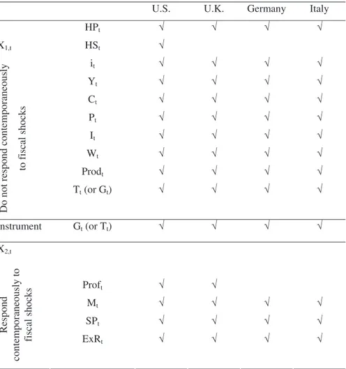
For the identification of the fiscal policy shocks, we use the following variables. The variables in X1t - the ones predetermined with respect to fiscal policy innovations -

are GDP, private consumption, GDP deflator, private investment, wages, and productivity. To these variables, we add for the housing price index (or the median sales price of new houses sold, in the case of the U.S.), the housing starts (only for the U.S.), and the average cost of government debt financing (or the yield to maturity of long-term government bonds). The variables in X2t – the ones allowed to react contemporaneously

to fiscal policy shocks – are the profits, and the money growth rate, to which we add the real exchange rate, the S&P500 Index (for the U.S.), the FTSE-All Shares Index (for the U.K.), and the MSCI index (for Germany and Italy). As measure of the fiscal policy instruments we use either the government expenditures (in which case, the government revenues are included in X1t) or the government revenues (in which case, the

government expenditures are included in X1t). We include a constant (or quarterly

seasonal dummies), and the government debt-to-GDP ratio in the set of exogenous variables. For Germany, we also consider two dummies: (i) one dummy for 1991:1, corresponding to the German reunification; and (ii) another dummy for 2000:3, to capture the spike in government revenue due to the sale of UMTS (Universal Mobile Telecommunications System) licenses.

independent restrictions and to get consistent impulse-responses (Christiano et al, 1999). As a result, the Choleski decomposition emerges as a particular case, where the restrictions are imposed such that ī0

Due to limitations of the data, housing starts are included only in the U.S. while, for Germany and Italy, profits are not included. For the U.K., we use the M4 growth rate

instead of the M2 growth rate. Table 1 shows for each country the list of variables

included in the estimation of the SVAR.

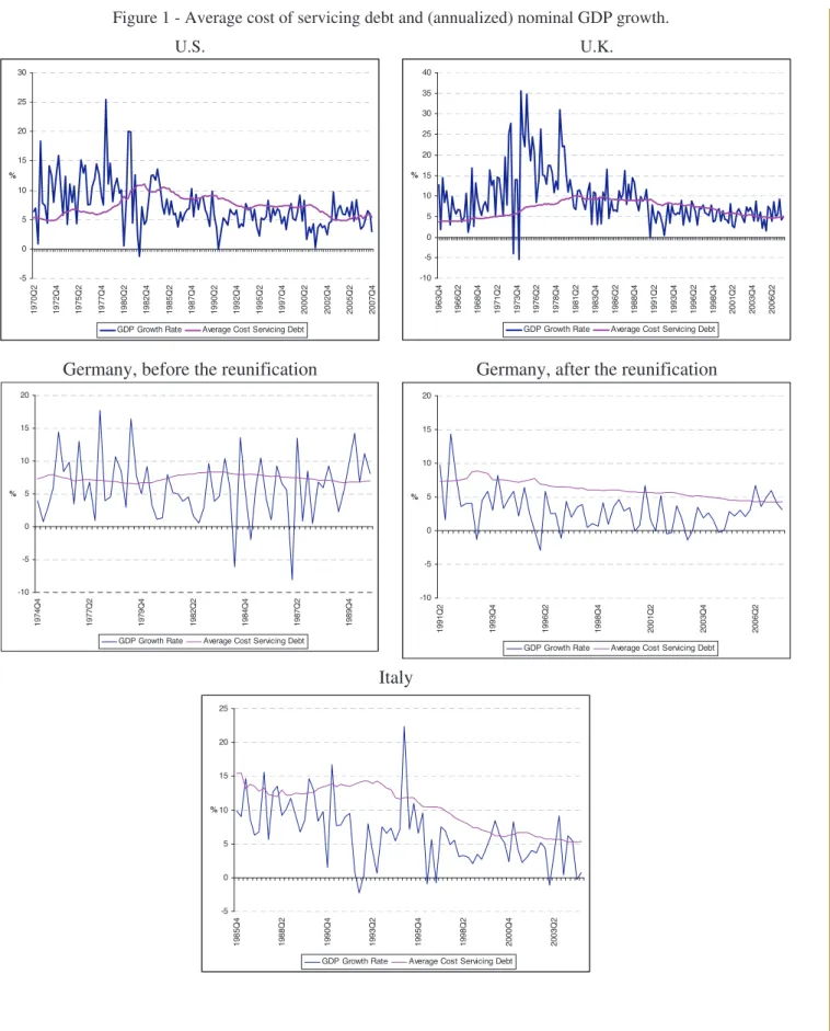
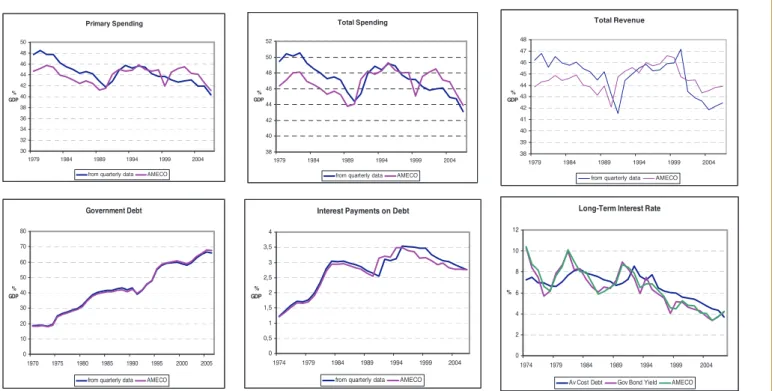
Among the set of variables included in the SVAR, the average government debt cost servicing deserves a special attention. We obtain the average implicit interest rate by dividing the net interest payments by the government debt at time tí1. Figure 1 plots the average debt cost servicing and the nominal (annualized) GDP growth for the U.S, the U.K., Germany, and Italy. It shows that countries have, in general, moved from a situation where nominal GDP growth exceeded the cost of financing the debt to a situation where the converse has been true.

The quarterly fiscal data refers to the Federal Government spending and revenue in the case of the U.S.A., and the Public Sector spending and revenue in the case of the U.K. In both cases, quarterly fiscal data is available directly from national accounts. As for Germany and Italy, we compute the quarterly series of government spending and revenue using the fiscal cash data, which is monthly published by the fiscal authorities of both countries. In this case, data for government spending and revenue refer to the Central Government and are available in a cash basis.

The data cover the following samples: 1970:3-2007:4, in the case of the U.S.A.; 1971:2-2007:4, in the case of the U.K.; 1979:2-2006:4, in the case of Germany; and 1986:2-2004:4, in the case of Italy.

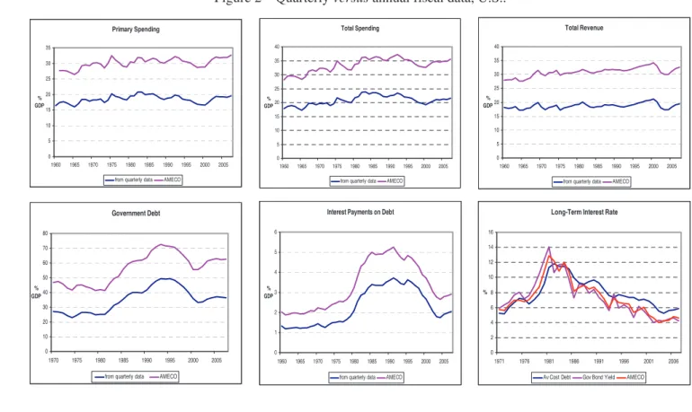
Figures 2, 3, 4, and 5 provide a comparison of the annual values of such quarterly fiscal data with the annual national accounts data provided by the European Commission (Ameco database). It is interesting to observe that the patterns of both series are rather similar.9 Moreover, in most of the cases, the levels themselves are also close.

Finally, Figure 6 plots the observed government debt-to-GDP ratio and the implicit debt-to-GDP ratio, that is, the one that would emerge by including the feedback from government debt. It shows that, despite some small discrepancies in the case of Italy, the implicit series for the debt-to-GDP ratio tracks pretty well the actual series. The small differences may be due to: (i) the consideration, in some cases, of the central

government revenues and expenditures instead of the general government revenues and expenditures; (ii) the use, for some countries, of the federal government debt instead of the general government debt; (iii) the presence of seigniorage, which is ignored in our framework; (iv) the fact that GDP growth rates and inflation rates are computed as logarithmic differences which can introduce some approximation errors; (v) the possible existence of stock-flow adjustments; and (vi) the inclusion of seasonally adjusted measures, namely, in the case of government revenues and expenditures.

Table 1 summarises the variables to be included in each country’s B-SVAR.

Table 1 – List of variables included in the B-SVAR.

U.S. U.K. Germany Italy

X1,t Do no t respond co nt empo raneo usly

to fiscal s

hocks HPt HSt it Yt Ct Pt It Wt Prodt

Tt (or Gt)

¥ ¥ ¥ ¥ ¥ ¥ ¥ ¥ ¥ ¥ ¥ ¥ ¥ ¥ ¥ ¥ ¥ ¥ ¥ ¥ ¥ ¥ ¥ ¥ ¥ ¥ ¥ ¥ ¥ ¥ ¥ ¥ ¥ ¥ ¥ ¥ ¥

instrument Gt (or Tt) ¥ ¥ ¥ ¥

X2,t Respond contem pora ne ousl y t o fiscal shoc

ks Proft

Mt SPt ExRt ¥ ¥ ¥ ¥ ¥ ¥ ¥ ¥ ¥ ¥ ¥ ¥ ¥ ¥

Note: HPt – housing price index; HSt – housing starts; it – average cost of refinancing debt

or yield to maturity of long-term government bonds; Yt – gross domestic product; Ct –

private consumption; Pt – GDP deflator; It – private investment; Wt – wages; Prodt –

productivity; Tt (or Gt) – government revenue (government spending); Gt (or Tt) –

government spending (government revenue); Proft – profits; Mt – monetary growth rate

(M2, for U.S., Germany and Italy; M4, for U.K.); SPt – stock prices; ExRt – effective

4.2 Results

The starting point is the estimation of a Bayesian Structural VAR (B-SVAR) that does not include the feedback from government debt, that is, where equation (2) is not considered. Then, we compare the results with the ones that emerge from estimating specifications (1), (2), and (3).

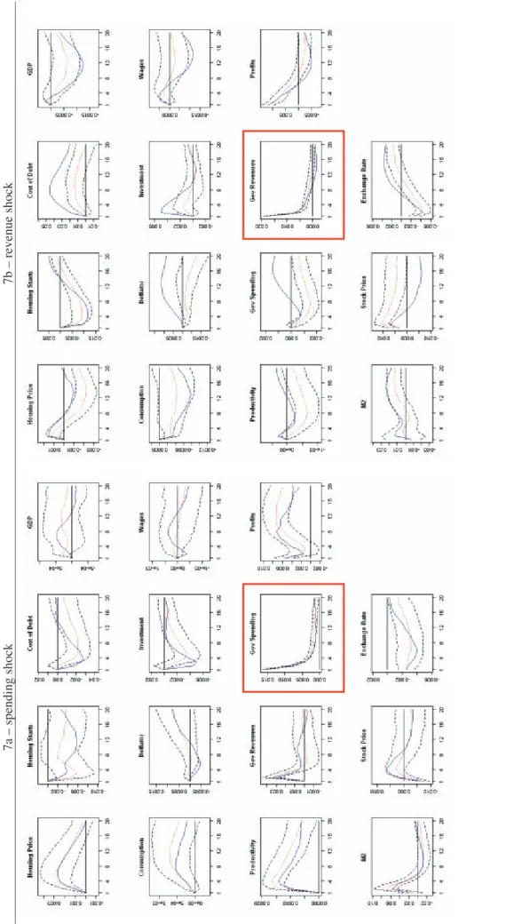
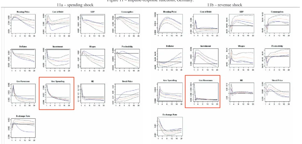
Figures 7, 9, 11, and 13 show the impulse-response functions to a fiscal policy shock. The solid line refers to the median response when the VAR is estimated without the government budget constraint, and the dashed lines are, respectively, the median response and the 68 percent posterior confidence intervals from the VAR estimated by imposing the government budget constraint. The confidence bands are constructed using a Monte Carlo Markov-Chain (MCMC) algorithm based on 500 draws.

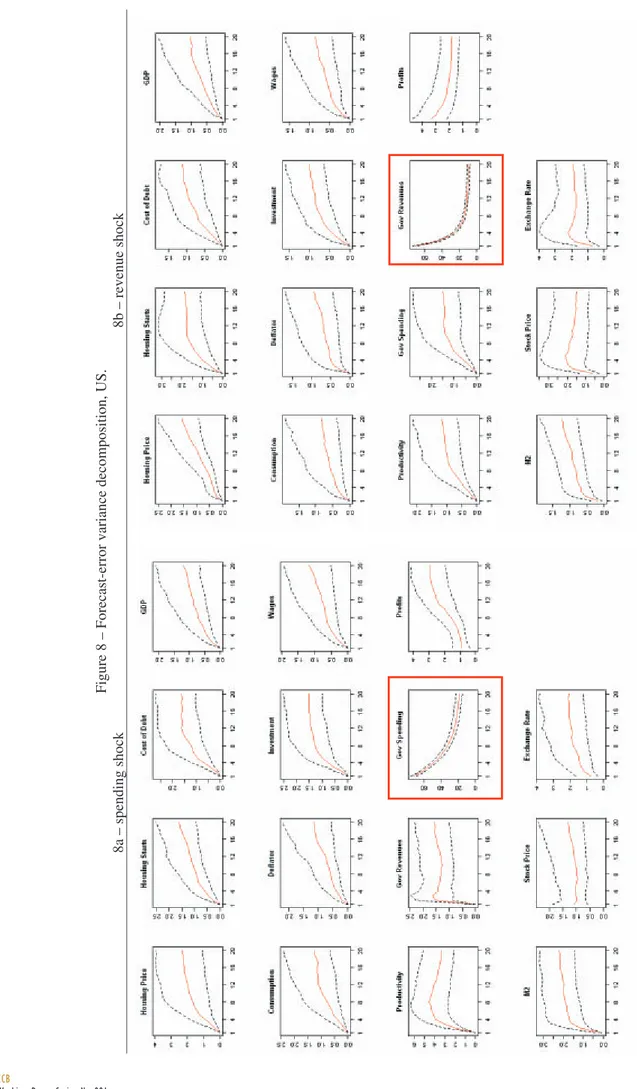
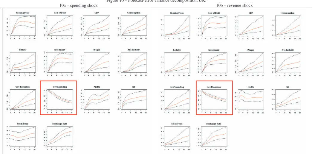
We also show in Figures 8, 10, 12, and 14 the forecast-error variance decompositions to a fiscal policy shock, imposing the budget constraint. The thinner line corresponds to the median estimate, and the dashed lines indicate the 68 percent posterior confidence intervals estimated by using a Monte-Carlo Markov-Chain algorithm based on 500 draws.

U.S.

Figure 7a displays the impulse-response functions of all variables in Xt to a

shock in government spending in the U.S.

In the case we do not include the debt feedback, it can be seen that government spending declines steadily following the shock, and it roughly vanishes after 6 quarters. The effects on GDP are small, positive, but not significant. However, they reveal a change in the composition of its major components: while government spending shocks do not seem to have an impact on private consumption, the effects on private investment are rather negative, supporting the idea of a “crowding-out” effect.10 In addition, there is a small and negative effect on the average cost of debt. In what concerns the reaction of asset markets, the empirical evidence suggests that while there is a positive effect on housing prices that persists for almost 12 quarters, the reaction of stock prices is rather small, negative and less persistent. Looking at the interaction between fiscal and

10 _{Fatás and Mihov (2001), when looking at the response to changes in different components of}

monetary policies, there is some support of the idea that an increase in government spending leads to a growth in the monetary aggregate, but the effect disappears after 4 quarters. Finally, the results suggest that after a government spending shock, the real effective exchange rate depreciates persistently for almost 12 quarters, although the magnitude is relatively small.

When we include the debt dynamics in the model, the effects of a government spending shock on GDP become smaller. Nevertheless, the effects on private investment remain negative while private consumption slightly increases, illustrating the wealth effects from government debt. On the other hand, and contrary to the previous findings, there is a small but negative effect on the average cost of refinancing the debt, which is eventually due to the rise in government revenues that follows the shock in government spending. The reaction of asset markets is similar to the model without the government constraint: there is a positive and persistent effect on housing prices, while the reaction of stock prices is smaller due to the debt dynamics and the portfolio reallocation.

Figure 7b shows the impulse-response functions to a shock in government revenue. The results suggest that government revenue declines steadily following the shock which erodes after 8 quarters. Contrary to a shock in government spending, the effects on GDP are negative, very persistent, and the trough is reached at after at after 10 quarters. They also reveal a change in the composition of GDP’s major components: while private consumption is negatively impacted by a positive shock in government revenues, the effect on private investment is roughly insignificant, despite a small positive initial reaction. That is, in this case, the “crowding-out” effect works mainly through the consumption channel. In what concerns the reaction of asset markets, the empirical evidence suggests that the effects of revenue shocks tend to be rather insignificant: despite a very small positive impact on housing and stock prices that persists for around 6 quarters, the effects then revert and disappear. Profits tend to fall after an initial increase while productivity is negatively affected by the shock. Finally, the results show that after a government revenue shock, the real effective exchange rate slightly appreciates.

Figure 8a plots the forecast error-variance decomposition of all variables in Xt to

majority of the variables. Similar conclusions can be drawn for the government revenue shock (Figure 8b).

U.K.

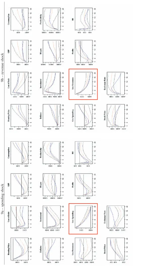
The impulse-response functions to a shock in government spending in the U.K are shown in Figure 9a.

While private consumption is not impacted by the spending shock, the effects on private investment are rather negative and very persistent, suggesting the idea of a “crowding-out” effect via investment. The dynamics of monetary aggregates suggest that M4 growth rate falls after the shock, supporting the idea of a monetary policy

tightening. Housing prices fall after the spending shock while stock prices decline only briefly. The effects on wages and productivity tend to be positive. Finally, the results suggest that after a government spending shock, the real effective exchange rate depreciates persistently for almost 20 quarters, in accordance with the findings for the U.S..

Figure 9b shows the impulse-response functions to a shock in government revenue. They support the idea of a “crowding-in” effect: private investment reacts positively to the shock. The effects on housing prices are also positive, but the reaction takes place with a lag of around 8 quarters. Although small in magnitude, the effects on profits are negative, while the national currency depreciates in real terms.

Figure 10a plots the forecast-error variance decomposition of all variables in the VAR to a shock in government spending. It shows that the shock accounts for 10% of the forecast-error variance of the exchange rate, 5% of the housing prices, and only 3% of stock prices.

Figure 10b displays the forecast-error variance decompositions and shows that government revenue shocks represents a large percentage (80%) of the forecast-error in government revenues and a small share of the forecast-error for the majority of the variables.

Germany

small in magnitude. Housing prices fall after around 10 quarters while stock prices drop immediately after the. Both productivity and wages fall with a lag of about 8 to 12 quarters.

When we include the feedback from the government debt, the cost of refinancing debt becomes positive, therefore, emphasizing the importance of account for debt dynamics.

Figure 11b plots the impulse-response functions to a shock in government revenue. Similarly to the U.S., the results show that government revenue declines quickly after the shock, eroding after 2 quarters.11 Contrary to the U.S., the effects on GDP are positive (although lagged in time. They support the idea of a “crowding-in” effect as both private consumption and private investment react positively to the shock. Revenue shocks tend to be significant and positive only for housing prices. The difference between the U.K. and the German experiences lies, therefore, on the balance between the magnitude of the credit channel and the “crowding-in” effect: in the U.K., the credit channel is reinforced by a “crowding-in” effect, and, therefore, a positive shock in government revenues has an impact of the same signal in housing prices; in Germany, the “crowding-in” effect is strong enough to compensate for the rise in the interest rates (credit channel). Note also that while in the U.K. the positive revenue shock is accompanied by a fall in government spending (therefore, justifying the fall of the interest rate), in the case of Germany the shock in government revenues is followed by a positive and persistent increase in government spending (consequently, explaining the rise of the interest rate).

The forecast-error variance decompositions to a shock in government spending and to a shock in government revenue are displayed, respectively, on Figures 12a and 12b. Shocks to spending also play an important role for the forecast-error of the price level (around 10%), GDP (9%), government revenue (7%) wages (close to 5%), housing prices (around 5%), and stock prices (5%). In contrast, revenue shocks explain only a negligible percentage of the forecast-error variance decomposition for the majority of the variables included in the system.

11 _{Afonso and Claeys (2008) mention that large revenue reductions unmatched by expenditure cuts have}

Italy

Finally, we look at the effects of a fiscal policy shock in Italy. Figure 13a displays the impulse-response functions to a shock in government spending. Despite a very small positive effect in the first quarters, GDP, private consumption, and private investment fall, suggesting a “crowding-out” effect. Government spending shocks have a positive and persistent effect on the price level. Housing prices seem to be positively affected by the shock, while stock prices fall for around 10 quarters.

Figure 13b shows the impulse-response functions to a shock in government revenue. The effects on GDP, private consumption, and private investment are negative, although not persistent as they vanish after 4 to 6 quarters. In consequence, and contrary to the U.K., they support the idea of a “crowding-out” effect. Regarding the reaction of asset markets, the empirical evidence shows that the effects of government revenue shocks tend to be positive for stock prices and negative for housing prices. This suggests that while the credit-channel (that is, the fall in interest rates) impacts positively in stock markets, for housing markets that channel is annihilated by the

wages and productivity increase, accompanying the rise of other macroeconomic variables. This partially explains why GDP, consumption and investment start recovering after around 8 quarters.

The error-forecast variance decompositions of all variables in Xt to a government

spending shock and a government revenue shock are plotted, respectively, in Figures 14a and 14b. They show that fiscal variables account for small percentages of the majority of the variables in the VAR. The only exception is the money growth rate, a feature that may be explained by the interaction between fiscal policy and monetary policy in the early sample observations.

4.3 Fiscal shocks and government debt feedback

We now consider the potential debt feedback and estimate the following structural VAR:

t t

i t

t X d d c

X * J H

*0 1 1 ... ( 1 *) , (7)

1 1

(1 )(1 )

t t t

t t

t t t t

i G T

d d

PY

S P

. (8)

debt ratio and allow us to take into account the debt feedback. Following Bohn (1998) and Favero and Giavazzi (2008), we model the target level of the debt as a constant on the basis of the evidence of stationarity of d. In addition, we impose the government’s intertemporal budget constraint as described by (8).

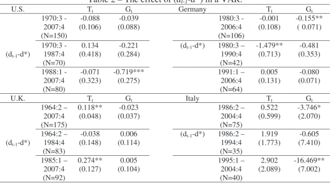
Table 2 reports the estimated coefficients on (dtí1 í d*) in the structural

equations of the SVAR (government spending and government revenue). We report the coefficients (and the standard errors in brackets) taken from the estimation for the full sample and for sub-samples. In the case of the U.S., we consider two sub-samples: 1970:3 – 1987:4, corresponding to the pre-Greenspan era; and 1988:1 – 2007:4, after Greenspan. In the case of the Germany, we also split the sample in two periods: 1980:3 – 1990:4, that is before the reunification; and 1991:1 – 2006:4, that is after the reunification. For the U.K. and Italy, each sub-sample is built by splitting the entire sample in roughly two sub-samples of similar size.

Table 2 – The effect of (dt-1-d*) in a VAR.

U.S. Tt Gt Germany Tt Gt

1970:3 - 2007:4 (N=150)

-0.088

(0.106) (0.088) -0.039 1980:3 - 2006:4 (N=106)

-0.001

(0.108) -0.155** (0.071)

(dt-1-d*)

1970:3 - 1987:4 (N=70)

0.134

(0.418) (0.284) -0.221 (dt-1-d*) 1980:3 1990:4 – (N=42)

-1.479**

(0.713) (0.353) -0.481 1988:1 -

2007:4 (N=80)

-0.071

(0.323) -0.719*** (0.275) 1991:1 2006:4 – (N=64)

0.005

(0.131) (0.071) -0.080

U.K. Tt Gt Italy Tt Gt

1964:2 – 2007:4 (N=175)

0.118**

(0.048) (0.037) -0.023 1986:2 – 2004:4 (N=75)

0.522

(0.599) -3.746* (2.070)

(dt-1-d*)

1964:2 – 1984:4 (N=83)

-0.038

(0.148) (0.114) 0.006 (dt-1-d*) 1986:2 1994:4 – (N=35)

1.919

(1.773) (7.410) -0.605 1985:1 –

2007:4 (N=92)

0.274**

(0.127) (0.104) 0.005 1995:1 2004:4 – (N=40)

2.902

(2.089) -16.469** (7.002)

Note: standard errors in brackets. *, **, *** - statistically significant respectively at the 10%, 5%, and 1% levels.

debt-to-GDP ratio is above its historical mean, government primary spending decreases (the coefficient associated to (dtí1 í d*) in the government spending equation is negative

and significant (-0.719).

For the U.K., the results show a stabilizing effect of the debt level on the primary budget balance that works mainly through the response of government revenues to deviations of the debt from the target level. This is, particularly, the case of the full sample and the second sub-sample (1985:1 – 2007:4). Therefore, when the debt ratio is above its sample mean, it is possible to observe an increase in government revenue (0.118, in the full sample; 0.274, for the second sub-sample).

In the case of Germany, there is evidence of a small stabilizing effect of the debt level on the primary surplus that works through the government spending (-0.155).

Finally, for Italy, one can see that when the debt ratio is above average, government spending strongly falls, particularly, in the period 1995:1-2004:4 where the coefficient associated to (dtí1í d*) is negative and large in magnitude (-16.469). This is

in line with the increase of fiscal policy imposed by the Maastricht Treaty.

5. Conclusion

This paper provides a detailed evaluation of the macroeconomic effects of fiscal policy.

We identify fiscal policy shocks using a recursive partial identification, and estimate a Bayesian Structural Vector Autoregression, therefore, accounting for the posterior uncertainty of the impulse-response functions. In addition, we explicitly include the feedback from government debt in our framework.

When the debt dynamics is explicitly taken into account, (long-term) interest rates and GDP become more responsive and the effects of fiscal policy on these variables also become more persistent.

Finally, the results provide weak evidence of stabilizing effects of the debt level on the primary budget balance.

A natural extension of the current work is related with the identification of the fiscal policy shocks. Blanchard and Perotti (2002) identify fiscal shocks by exploiting decision lags in fiscal policymaking. This approach assumes that: (i) discretionary government purchases and revenues are predetermined with respect to the macroeconomic variables; and (ii) it uses information about the elasticity of fiscal variables to economic activity which enables to identify the automatic response of fiscal policy. In this context, Afonso and Sousa (2008) include an identification of the automatic response of fiscal policy to macroeconomic variables such as GDP, deflator, or interest rate. Whilst narrower in scope – as its goal is solely to understand the linkages between fiscal policy and asset markets – than the present work, the estimation of a fully simultaneous system of equations in a Bayesian framework can prove to be a useful alternative approach, while allowing to assess the robustness of the effects of fiscal policy on asset markets.

References

AFONSO, A. (2008a), “Euler testing Ricardo and Barro in the EU”, Economics

Bulletin, 5 (16), 1-14.

AFONSO, A. (2008b), “Ricardian Fiscal Regimes in the European Union”, Empirica, 35 (3), 313–334.

AFONSO, A. (2008c), “Expansionary fiscal consolidations in Europe: new evidence”,

Applied Economics Letters, DOI http://dx.doi.org/10.1080/13504850701719892,

forthcoming.

AFONSO, A.; CLAEYS, P. (2008), “The dynamic behaviour of budget components and output”, Economic Modelling, 25, 93-117.

AFONSO, A.; SOUSA, R. M. (2008), “Fiscal policy, housing and stock prices”, ECB Working Paper, forthcoming.

AFONSO, A.; STRAUCH, R. (2007), “Fiscal policy events and interest rate swap spreads: some evidence from the EU”, Journal of International Financial Markets,

AIYAGARI, R.; CHRISTIANO, L.; EICHENBAUM, M. (1990), “Output, employment and interest rate effects of government consumption”, Journal of Monetary

Economics, 30, 73–86.

ALESINA A.; ARDAGNA, S. (1998), “Tales of fiscal adjustment”, Economic Policy, 27, 489-545.

AOKI, K.; PROUDMAN, J.; VLIEGHE, G. (2004), "House prices, consumption, and monetary policy: a financial accelerator approach", Journal of Financial

Intermediation, 13, 414-435.

BARRO, R. J. (1974), "Are government bonds net wealth?", Journal of Political

Economy , 82(6), 1095-1117.

BAUWENS, L.; LUBRANO, M.; RICHARD, J.-F. (1999), Bayesian inference in

dynamic econometric models, Oxford University Press, Oxford.

BAXTER, M.; KING, R. (1993), “Fiscal policy in general equilibrium”, American

Economic Review, 83, 315–334.

BEETSMA, R.; JENSEN, H. (2005), “Monetary and fiscal policy interactions in a Micro-Founded Model of a Monetary Union”, Journal of International Economics, 67, 320-352.

BERNANKE, B.; KUTTNER, K. (2005), "What explains the stock market's reaction to Federal Reserve policy?", Journal of Finance, 60(3), 1221-1257.

BERNOTH, K. J.; VON HAGEN, J.; SCHUKNECHT, L. (2003), “The determinants of the yield differential in EU government bond market”, ZEI – Center for Eurpean Integration Studies, Working Paper.

BIAU, O.; GIRARD, E. (2005), “Politique budgétaire et dynamique économique en France: l'approche VAR structurel.”, Économie et Prévision, 169–171, 1–24.

BLANCHARD, O. (2003), Macroeconomics, 3rd ed., Prentice Hall.

BLANCHARD, O.; PEROTTI, R. (2002), "An empirical characterization of the dynamic effects of changes in government spending and taxes on output", Quarterly

Journal of Economics, 117(4), 1329-1368.

BOHN, H. (1998), "The Behaviour of U.S. public debt and deficits", Quarterly Journal

of Economics, 113, 949-963.

BROOK, A.-M. (2003), “Recent and prospective trends in real long-term interest: fiscal policy and other drivers”, OECD Working Paper #21.

CHIRINKO, R.; de HAAN, L.; STERKEN, E. (2004), "Asset price shocks, real expenditures, and financial structure: a multi-country analysis", Emory University, Working Paper.

CHRISTIANO, L.; EICHENBAUM, M. (1992), “Current real business cycles theories and aggregate labor market fluctuations”, American Economic Review, 82, 430–450. CHRISTIANO, L. J.; EICHENBAUM, M.; EVANS, C. L. (2005), "Nominal rigidities

and the dynamic effects of a shock to monetary policy", Journal of Political

Economy, 113(1), 1-45.

CHRISTIANO, L. J.; EICHENBAUM, M.; EVANS, C. L. (1999), "Monetary policy shocks: what have we learned and to what end?", in TAYLOR, J.; WOODFORD, M., eds, Handbook of Macroeconomics, 1A, Elsevier, Amsterdam.

CHUNG, H.; LEEPER, D. (2007), “What has financed government debt?”, NBER Working Paper #13245.

CHUNG, H.; DAVIG, T.; LEEPER, E. M. (2007), “Monetary and fiscal switching”,

Journal of Money, Credit and Banking, 39(4), 809-842.

CODOGNO, L.; FAVERO, C.; MISSALE, A. (2003), “Yield spreads on EMU government bonds”, Economic Policy, 37, 503-532.

CORSETTI, G.; MÜLLER, G. J. (2006), “Twin deficits: squaring theory, evidence and common sense”, Economic Policy, 21(48), 597-638.

CRAINE, R.; MARTIN, V. (2003), "Monetary policy shocks and security market responses", University of California at Berkeley, Working Paper.

DAVIG, T.; LEEPER, E. M. (2005), “Fluctuating macro policies and the fiscal theory”, NBER Working Paper #11212.

DE CASTRO FERNÁNDEZ, F.; HERNÁNDEZ DE COS, P. (2006), “The economic effects of exogenous fiscal shocks in Spain: a SVAR approach”, ECB Working Paper #647.

EDELBERG, W.; EICHENBAUM, M.; FISHER, J. (1999), “Understanding the effects of a shock to government purchases”, Review of Economics Dynamics, 2, 166–206. ENGEN, E. M.; HUBBARD, R. G. (2004), “Federal government debt and interest

rates”, NBER Working Paper #10681.

FATÁS, A.; MIHOV, I. (2001), “The effects of fiscal policy on consumption and employment: theory and evidence”, CEPR Discussion Paper # 2760.

FAVERO, C.; GIAVAZZI, F. (2008), "Debt and the effects of fiscal policy", University of Bocconi, Working Paper.

FERRERO, A. (2006), “Fiscal and monetary rules for a currency union”, New York University, manuscript.

GALE, W. G.; ORSZAG, P. R. (2003), “Economic effects of sustained budget deficits”,

National Tax Journal, 56, 463-485.

GALE, W. G.; ORSZAG, P. R. (2002), “The economic effects of long-term fiscal discipline”, Urban-Brookings Tax Policy Center, Discussion Paper.

GALI, J.; MONACELLI, T. (2008), “Optimal monetary and fiscal policy in a currency union”, University of Bocconi, manuscript.

GALI, J.; PEROTTI, R. (2003), “Fiscal policy and monetary integration in Europe”, University of Pompeu Fabra, Working Paper.

GALI, J.; VALLÉS, J.; LÓPEZ-SALIDO, J. D. (2007), “Understanding the effects of government spending on consumption”, Journal of the European Economic

Associaton, 5(1), 227-270.

GIAVAZZI, F.; PAGANO, M. (1990), “Can severe fiscal contractions be expansionary? Tales of two small european countries”, in BLANCHARD, O. J.; FISCHER, S. (eds.), NBER Macroeconomics Annual, MIT Press, 75–110.

GIAVAZZI, F.; JAPPELLI, T.; PAGANO, M. (2000), "Searching for non-linear effects of fiscal policy: evidence from industrial and developing countries", European

Economic Review, 44(7), 1259-1289.

GIORDANO, R.; MOMIGLIANO, S.; NERI, S.; PEROTTI, R. (2007), “The effects of fiscal policy in Italy: Evidence from a VAR model”, European Journal of Political

Economy, 23, 707-733.

GOODHART, C.; LEMMEN, J. J. G. (1999), “Credit risks and european government bond markets: a panel data econometric analysis”, Eastern Economic Journal, 25(1), 77-107.

HEPPKE-FALK, K.H.; HÜFNER, F. (2004), “Expected budget deficits and interest rate swap spreads – evidence for France, Germany and Italy”, Deutsche Bundesbank, Discussion Paper #40.

IACOVIELLO, M. (2005), "House prices, borrowing constraints, and monetary policy in the business cycle", American Economic Review, 95(3), 739-764.

IACOVIELLO, M.; MINETTI, R. (2003), "The credit channel of monetary policy: evidence from the housing market", Boston College, Working Paper.

IACOVIELLO, M.; NERI, S. (2007), "The role of housing collateral in an estimated two-sector model of the US economy", Boston College, Working Paper.

JULLIARD, C.; MICHAELIDES, A.; SOUSA, R. M. (2008), "Housing prices and monetary policy", London School of Economics and Political Science, Working Paper.

KIM, J.-Y. (1994), "Bayesian asymptotic theory in a time series model with a possible nonstationary process", Econometric Theory, 10(3), 764-773.

KIM, S.; ROUBINI, N. (2003), “Twin deficits or twin divergence? Fiscal policy, current account, and the real exchange rate in the U.S.”, New York University, manuscript.

KORMENDI, R. C. (1983), “Government debt, government spending, and private sector behavior”, American Economic Review, 73, 994-1010.

LAUBACH, T. (2003), “New evidence on the interest rate effects of budget deficits and debt”, Board of Governors of the Federal Reserve System, Finance and Economics Discussion Paper #12.

MCCARTHY, J.; PEACH, R. (2002), "Monetary policy transmission to residential investment", Federal Reserve Bank of New York Economic Policy Review, 8(1), 139-158.

MONACELLI, T.; PEROTTI, R. (2006), "Fiscal policy, the trade balance, and the real exchange rate: implications for international risk sharing", University of Bocconi, manuscript.

MOUNTFORD, A.; UHLIG, H. (2005), "What are the effects of fiscal policy shocks?", Humboldt-Universität zu Berlin Working Paper SFB #649.

PÉREZ, J. (2007), “Leading indicators for euro area government deficits”, International

Journal of Forecasting, 23, 259-275.

PEROTTI, R. (1999), “Fiscal policy in good times and bad”, Quarterly Journal of

Economics, 114, 1399-1436.

RAMEY, V.; SHAPIRO, M. (1998), “Costly capital reallocation and the effects of government spending”, Carnegie Rochester Conference on Public Policy, 48, 145-194.

RIGOBON, R.; SACK, B. (2003), "Measuring the reaction of monetary policy to the stock market", Quarterly Journal of Economics, 118(2), 639-670.

RIGOBON, R.; SACK, B. (2002), "The impact of monetary policy on asset prices", Finance and Economics Discussion Series 2002-4, Board of Governors of the Federal Reserve System.

ROMER, C.; ROMER, D. H. (2007), "The macroeconomic effects of tax changes: estimates based on a new measure of fiscal shocks", NBER Working Paper #13264. SCHERVISH, M. J. (1995), Theory of statistics, Springer, New York.

SIMS, C.; ZHA, T. (1999), "Error bands for impulse-responses", Econometrica, 67(5), 1113-1155.

UPPER, C.; WORMS, A. (2003), “Real long-term interest rates and monetary policy: a cross-country perspective”, BIS Papers, 19, 234-257.

ZELLNER, A. (1971). An introduction to bayesian inference in econometrics, Wiley, New York.

Appendix A. The government’s intertemporal budget constraint

The government’s intertemporal budget constraint can be written as: )

( ) 1

( t t 1 t t

t i B G T

B

where Bt represents the stock of debt at the end of period t, Bt-1 is the stock of debt at the

end of period t-1, Gt is the government primary spending during the period t, Tt is the

government revenue during the period t, and i is the nominal interest.

Dividing both sides of the last identity by the nominal GDP, PtYt, where Pt is the

general price level, and Yt represents the real GDP, one obtains:

t t t t t t t t t t t Y P T G Y P B i Y P

B ( )

) 1

( 1 _.

Finally, noting that

» ¼ º « ¬ ª x ) 1 )( 1 ( 1 1 1 1 1 1 1 1 1 1 t t t t t t t t t t t t t t t Y P B Y P Y P Y P B Y P B P S

where St, and Pt, represent, respectively, the inflation rate and the growth rate of real

GDP, and defining by lowercase letters the variables expressed as ratio of GDP, that is

t t t t Y P B

d : ;

1 1 1 1: t t t t Y P B d ; t t t t Y P G

g : ; and

t t t t Y P T t :

) ( ) 1 )( 1 ( ) 1 (

1 t t

t t t

t

t d g t

i d P S .

This is identical to equation (2) in the text.

Appendix B. Confidence bands of the impulse-response functions

The impulse-response function to a one standard-deviation shock under the normalization of / I is given by:

. ) ( 1 0 1 _* L

B (B.1)

To assess uncertainty regarding the impulse-response functions, we follow Sims and Zha (1999) and construct confidence bands by drawing from the Normal-Inverse-Wishart posterior distribution of B(L) and Ȉ

) ) ' ( , ( ~

| ^ 1

6 1 E 6… X X

E (B.2)

) , ) (( Wishart

~ ^ 1

1 _{T6 T m}

6 _(B.3)

where ȕ is the vector of regression coefficients in the VAR system, Ȉ is the covariance matrix of the residuals, the variables with a hat denote the corresponding maximum-likelihood estimates, X is the matrix of regressors, T is the sample size and m is the number of estimated parameters per equation (see Zellner, 1971; Schervish, 1995; and Bauwens et al., 1999).

Appendix C. Data description and sources

C.1 U.S. Data

Housing Sector

Housing prices are measured using two sources: (a) the Price Index of New One-Family Houses sold including the Value of Lot provided by the U.S. Census, an index based on houses sold in 1996, available for the period 1963:1-2006:3; and (b) the House Price Index computed by the Office of Federal Housing Enterprise Oversight (OFHEO), available for the period 1975:1-2007:4. Data are quarterly, seasonally adjusted.

Housing Market Indicators

Other Housing Market Indicators are provided by the U.S. Census. We use the Median Sales Price of New Homes Sold including land and the New Privately Owned Housing Units Started. We seasonally adjust quarterly data for the Median Sales Price of New Homes Sold including land using Census X12 ARIMA, and the series comprise the period 1963:1-2007:4. The data for the New Privately Owned Housing Units Started are quarterly (computed by the sum of corresponding monthly values), seasonally adjusted and comprise the period 1959:1-2007:4.

GDP

The source is Bureau of Economic Analysis, NIPA Table 1.1.5, line 1. Data for GDP are quarterly, seasonally adjusted, and comprise the period 1947:1-2007:4.

Consumption

non-durable consumption goods (line 3) and services (line 4). Data are quarterly, seasonally adjusted, and comprise the period 1947:1-2007:4.

Price Deflator

All variables were deflated by the GDP deflator. Data are quarterly, seasonally adjusted, and comprise the period 1967:1-2007:4. The source is the Bureau of Economic Analysis, NIPA Tables 1.1.5 and 1.1.6, line 1.

Investment

The source is Bureau of Economic Analysis, NIPA Table 1.1.5. Investment is defined as the gross private domestic investment (line 6) excluding residential investment (line 11). Data are quarterly, seasonally adjusted, and comprise the period 1947:1-2007:4.

Wages

The source is Bureau of Economic Analysis, NIPA Tables 2.1 and 2.6. Wages are defined as the sum of wages and salary disbursements (line 3). Data are quarterly, seasonally adjusted, and comprise the period 1947:1-2007:4.

Productivity

Productivity is defined as the Nonfarm Business Output Per Hour Index (1992=100) ("PRS85006093"). Data are quarterly, seasonally adjusted, and comprise the period 1947:1-2007:4. The source is the Bureau of Labour Statistics.

Profits

The source is Bureau of Economic Analysis, NIPA Table 1.14. Profits are defined as the profits before tax without IVA and CCAdj ("A446RC1", line 32). Data are quarterly, seasonally adjusted, and comprise the period 1947:1-2007:4.

Monetary Aggregate

Monetary Aggregate corresponds to M2. Data are quarterly, seasonally adjusted, and

comprise the period 1960:1-2007:4. The sources are the OECD, Main Economic Indicators (series "USA.MABMM201.STSA") and the Board of Governors of the Federal Reserve System, Release H6.

Stock Market Index

Stock Market Index corresponds to S&P 500 Composite Price Index (close price adjusted for dividends and splits). Data are quarterly (computed from monthly series by using end-of-period values), and comprise the period 1950:1-2007:4.

Exchange Rate

The source is the Bank for International Settlements (BIS). Exchange Rate corresponds to real effective exchange rate (series “RNUS”). Data are quarterly (computed from monthly series by using end-of-period values), and comprise the period 1964:1-2007:4.

Government Spending

Government Revenue

The source is Bureau of Economic Analysis, NIPA Table 3.2. Government Revenue is defined as government receipts at annual rates (line 36). Data are quarterly, seasonally adjusted, and comprise the period 1947:1-2007:4.

Debt

Debt corresponds to the Federal government debt held by the public. The source is the Federal Reserve Bank of St Louis (series “FYGFDPUN”). Data are quarterly, seasonally adjusted, and comprise the period 1970:1-2007:4.

Average Cost of Financing Debt

The average cost of financing debt is obtained by dividing net interest payments by debt at time t-1.

Long-Term Interest Rate

Long-Term Interest Rate corresponds to the yield to maturity of 10-year government securities. Data are quarterly, and comprise the period 1960:1-2007:4. The source is the OECD, Main Economic Indicators (series "USA.IRLTLT01.ST").

C.2 U.K. Data

Housing Prices

Housing prices are measured using two sources: (a) the Mix-Adjusted House Price Index (Feb 2002 = 100) provided by the Office of the Deputy Prime Minister (ODPM), seasonally adjusted, and available for the period 1968:2-2007:4; and (b) the All-Houses Price Index (1952Q4 = 100 and 1993Q1=100) computed by the Nationwide Building Society, which we seasonally adjust using Census X12 ARIMA, and is available for the period 1952:4-2007:4.

GDP

Data for GDP are quarterly, seasonally adjusted, and comprise the period 1955:1-2007:4. The source is the Office for National Statistics, Release UKEA, Table A1 (series "YBHA").

Consumption

The source is the Office for National Statistics, Release CT, Tables 0.GS.CS, SER.CS and NDG.CS. Consumption is defined as the expenditure in non-durable consumption goods and services excluding housing services, actual rentals paid by tenants and imputed rentals for housing, i.e. UTIJ-[LLKE-(UTZI+ZWUQ)]+UTIN-(BMBT-GBFJ), where: "UTIJ" is expenditure in non-durable goods, "LLKE" is expenditure in housing, water, electricity, gas and other fuels, "UTZI" is expenditure in water supply, "ZWUZQ" is expenditure in electricity, gas and other fuels, "UTIN" is expenditure in consumption services, "BMBT" is expenditure in actual rentals paid by tenants, and "GBFJ" is expenditure in imputed rentals for housing. Data are quarterly, seasonally adjusted, and comprise the period 1963:1-2007:4.

Price Deflator

Investment

The source is the Office for National Statistics, Release MD (Table 1.10) and Release ETAS (Table 2.7). Investment is defined as total gross fixed capital formation (series "NPQX") excluding gross fixed capital formation in dwellings by private sector (series "DFDF") and gross fixed capital formation by general government (series "NNBF"). Data are quarterly, seasonally adjusted, and comprise the period 1955:1-2007:4.

Wages

Wages correspond to U.K. average monthly wages (2000=100). Data are quarterly, seasonally adjusted, and comprise the period 1963:1-2007:4. The source is Datastream, based on IMF, International Financial Statistics.

Productivity

The source is the Office for National Statistics, Release PRDY (Table 1) and Release MDS (Table 7.2). Productivity is defined as the Index of Output per worker of the whole economy (2003=100) (series "A4YM"). Data are quarterly, seasonally adjusted, and comprise the period 1959:3-2007:4.

Profits

The source is the Office for National Statistics, Release UKEA, Tables X1 and X8. Profits are defined as the sum of gross trading profits of private non-financial corporations both non UKs (series "CAED") and UK continental shelf companies (series "CAGD") and financial corporations (series "RITQ"). Data are quarterly, seasonally adjusted, and comprise the period 1955:1-2007:4.

Monetary Aggregate

The source is the Office for National Statistics, Release MD, Table 17.5. Monetary Aggregate corresponds to: (a) M2 (series "VQWU"); and (b) M4 (series "AUYN"). Data

are quarterly, seasonally adjusted, and comprise the periods 1982:3-2007:4 (for M2) and

1963:1-2007:4 (for M4).

Stock Market Index

Stock Market Index corresponds to the FTSE-All Shares Index (1962:2=100 or 1962 April=100). Data are quarterly, and comprise the period 1962:2-2007:4. The source is Datastream.

Exchange Rate

The source is the Bank for International Settlements (BIS). Exchange Rate corresponds to real effective exchange rate (series “RNGB”). Data are quarterly (computed from monthly series by using end-of-period values), and comprise the period 1964:1-2007:4.

Government Spending