Finite element formulation and analysis of a functionally graded Timo- shenko beam subjected to an accelerating mass including inertial effects of the mass

(1)

Finite element formulation and analysis of a functionally graded

Timo-shenko beam subjected to an accelerating mass including inertial effects of

the mass

Abstract

This study describes a new finite element method that can be used to analyse transverse and axial vibrations of a Functionally Graded Material (FGM) beam under an accelerating / decelerating mass. The differential equations of the FGM beam are obtained using First-order Shear Deformation Theory (FSDT). In these equations, the interaction terms of mass inertia are derived from the second-order exact differentiation of displacement functions with respect to mass contact point. The FGM beam is made of two different materials (Steel and Alumina Al2O3),

which vary in thickness with a power law. Including the effects of neutral axis shift and mass inertia, the proposed method can be used when the dynamic be-haviour of the FGM Timoshenko beams is to be analysed in transverse and axial directions, depending on the interaction with the acceleration of the moving loads. After validating this work with literature studies, new investigations and findings are presented for both moving load and mass assumptions. In addition, the obtained results of Timoshenko Beam (TBT) and Euler Bernoulli beam the-ory (EBT) are compared for FGM beams with various speeds and accelerations of moving mass.

Keywords

FGM beams, Finite element, moving load, mass inertia, accelerating

1 INTRODUCTION

In recent years, there has been a new class of composite materials known as Functionally Graded Materials (FGMs), where different components of materials are graded continuously under a force law. This nonhomogeneous composite new material is an alternative to stress concentrations in conventional composite structures where the laminates have very different mechanical and thermal properties. In FGM, the proportions of constituent materials are slowly changed volu-metrically to remove the interfacial effects of thermal and mechanical stresses. In some engineering applications, materials are expected to withstand high temperatures under severe loading conditions. Because of better thermal resistance, the properties of the ceramic component can withstand high temperature environments, while the metal component in the functionally graded materials (FGMs) provides more mechanical strength to reduce fracture performance probability. In defense, aviation and aerospace, automotive, transportation systems and similar engineering applications, the FGMs have the ability to combine many different properties such as thermal and mechanical strength, structural lightness and wear resistance. It is expected that the use of FGMs in engineering applications will increase as the production opportunities with the developing technology increase. A wide range of FGM application systems are support systems such as beams. In recent years, many scientists have studied the static and vibrational behaviour of FGM beams (Aydogdu and Taskin, 2007; Chakraborty et al., 2003; Ebrahimi et al., 2016; Eltaher et al., 2013; Jafari-Talookolaei et al., 2018; Kang and Li, 2010; Khan et al., 2016; Kim and Lee, 2014; Kosmatka, 1995; Lien et al., 2017; Mashat et al., 2014; Masoodi and Moghad-dam, 2015; Murín et al., 2010; Nguyen and Nguyen, 2015; Rezaiee-Pajand et al., 2018; Rezaiee-Pajand and Masoodi, 2016; Rezaiee-Pajand and Rajabzadeh-Safaei, 2018; Sina et al., 2009; Taati, 2018; Taeprasartsit, 2013; Yokoyama, 1996; Zhang and Zhou, 2008). Analysis of systems subjected to moving loads, an ongoing long-standing problem, and some studies have investigated the transverse responses of the limited number of FGM beams to moving forces, in the transverse and axial directions, neglecting the effects of inertia (Kadivar and Mohebpour, 1998; Nguyen et al., 2013; Rajabi et al., 2013; _Şim_şek and Al-shujairi, 2017; _Şim_şek and Kocatürk, 2009). Other studies of moving loads at constant and variable speeds have also investigated the transverse responses of beams and plates with uniform cross-section and homogeneous materials (Kadivar and Mohebpour, 1998; Michaltsos, 2002; Wang, 2009; Yoshida and Weaver, 1971). Considering the

İsmail ESENa Mehmet Akif KOÇb

* Yusuf ÇAYb

a

Department of Mechanical Engineering, Karabük University, Karabük, Turkey. E-mail: iesen@kara-buk.edu.tr

b

Department of Mechatronics Engineering, Sakarya University, Sakarya, Turkey. E-mail: makoc@sa-karya.edu.tr, ycay@sakarya.edu.tr

*Corresponding author

http://dx.doi.org/10.1590/1679-78255102

(2)

inertia effect of mass, some analytical and finite element studies of moving mass for beams and plates are given in (Cifuentes, 1989; Esen, 2013; Meirovitch, 1967; Wu, 2005).

The calculation methods given in the literature for FGM beams in general are for low speed load movements and simplified conditions where the convective acceleration effect of moving load mass is neglected. In this study, a more realistic modelling and analysis method of such systems is provided without neglecting the Coriolis, inertia and centrifugal effects of the moving load accelerating along the deflected shape of the FGM beams. The natural vibration frequencies are important in the dynamic behavior of FGM and other beams. For this reason, any factor that affects or alters the frequency of the beam in the dynamic interaction is also very important. This is also the reason why the inertia effect of mass should be involved in the dynamic interaction of moving mass and beam, and in this study, this behavior is examined in this context in order to better understand the dynamic behavior. In addition to transverse vibration, axial vibration is also induced by inertia effects of the mass of the load in the conditions of rapid acceleration and panic braking, which have been often neglected in the literature. Moreover, this work also presents a detailed comparison of moving load and moving mass assumptions for FGM beams, including differences between Timoshenko (TBT) and Euler-Bernoulli beam theories (EBT).

2 MATHEMATICAL MODELLING

Figure 1 shows a FGM beam of length L exposed to a mass, moving from left to right with a variable speed. The modelling of the finite elements over the length is considered to have n beam elements with n + 1 nodes. The two nodes of each beam element have three displacements and forces at each node. Where xp is the time-dependent global position

of the moving mass, and xm is the local coordinate of the mass measured from the left end of the element. A rectangular

section with width b and height h and a material for the beam is considered to be a FGM consisting of two basic materials and it is assumed that effective material properties are distributed in the direction of thickness (z-direction) according to a power law as:

1

( ) ( ) , ( ) , 1

2

n n

b t b t t b

z z

P z P P P V z V V

h h

 _  _

 _  _

   _ __ _  __  

 

    (1)

In Eq. (1) P(z) signifies the effective material properties, including mass density, Young's modulus, shear modulus and Poisson ratios; Pt and Pb are the material properties of the material at the top and bottom surfaces, respectively; Vt and

Vb respectively be the volume fractions of the materials at the top and bottom surfaces; n is the non-negative power-law

index, expresses the distribution of the constituent materials. Figure 2 depicts the change in volume fraction along the beam thickness for various index values of the FGM beam.

X,u

Z,w

x

p

(t)

m

p

_v(t)

L,



_b

,



t

, E

b

,

E

t

,G

b

,G

t

,



b



t

h

o

s

x

m

Figure 1: A thick FGM beam under the influence of a moving point mass.

Due to variation of the effective Young's modulus, the neutral axis is no longer at the mid-plane thus, the shift of the neutral axis can be decided by solving the following equation (Eltaher et al., 2013; Zhang and Zhou, 2008).











/2 /2 0 /2 /2 ) ( 2 ( ) 2 h

h t b

h

t b

h

zE z dz _E _{E hn}

z

E E n

E z zd n

      



(2)

Where z0 is the geometric neutral axis shift and h is the thickness of the beam, the position of the physical neutral axis

depends on the ratio between the Et / Eb of the Young modules and the power law index n of the material components.

(3)

/ Eb ratio. In the figure, the shift increases with increasing Et / Eb ratio, but decreases as n index increases. Here indices t

and b, respectively, stand for top surface (ceramic) and bottom surface (metal).

Figure 2: a) Effect of the power law index on the physical neutral axis position. b) Variation in volume fraction in the thickness of FGM beams depending on the power-law exponent n.

In the formulation, the following assumptions will be assumed (Figure 1): inertia effects of mass will take part in the calculations, and the moving mass will always be in contact with the beam, separation not allowed. When a FGM beam is considered in a coordinate system (x, z) where the x-axis coincides with the physical neutral axis of the beam as shown in Fig. 1, by adopting the FSDT and by including the axial force at the contact point with the beam, the displacements at any point of the beam become:

( , , ) ( , ) ( , ), ( , , ) ( , )

u x z t u x t z x t w x z t w x t (3)

Where u x t( , ), w x t( , ) and ( , )x t are the axial, transverse displacement and rotation of the cross section at point x on the physical neutral axis, Considering FSDT the strains and stresses related to the displacement field in Eq. (3) are given by

;

( ) , ( )

xx xz

xx xx xz xz

u w

z u z w

x x x

E z G z



    

    

  _ _  _

       

  

 

(4)

Where  is the surface correction factor. From Eq. (4), the strain energy of the beam is given by

2 2 2

11 12 22 33

0

1 ₎

2 1

2

xx xx xz xz V

l

U dV

D u D u D D w dx

   

   

 

 _ _{ } _ _ 

 _     _

 



(5)

Where D11 is the axial, D12 is the axial-rotational, D22 is the bending, and D33 is the shear rigidities, respectively and

computed as

2

11, 12, 22 _A(1, , ) ( ) , 33 _A ( )

D D D 

_

z z E z dA D 

_

G z dA (6)

The kinetic energy resulting from the equation (3) is

2 2 2

11 22 12

0

1 ₍ ₎ ₂

2 L

T  _I u w I   I u dx_

 



_ _  _ (7)

(4)

0 0

2 11 12 22

2 2

0 0

( , , ) ( )(1, , )

( ) (1, , )( ) (1, , )( )

A

h h h

I I I z z z dA

b x z z h z dz z z h z dz

                    



(8)

The potential energy of the moving mass including convective acceleration is given by

( , ) ( , ) ( ( )) ( , ) ( , ) ( ( ))

p p p p p p

V m g__ w x t w x t __  xx t m a__ u x t u x t __ xx t (9)

Where g is gravitational acceleration, δ(.) is the Dirac delta function,

m w x t

_p



( , )

_p and

m u x t

_p



( , )

_p are inertia forces in z and x direction respectively,

x t

_p

( )

is the function describing the motion of the mass at time t, and given by









2 2 2

0 0

( ) 0.5 , d / d ; d / d

p p

p _{x x} _{x x}

x t x v t at v x t a x t

 

     (10)

with x0 and v0 are initial position and velocity while a denotes the acceleration of the mass. Using Hamilton’s principle,

Eqs. (5), (7) and (9) lead to the resulting coupled governing differential equations

11 12 11 12

2 11 33

22 12 12 22 33

0

( ) ( 2

) 0

( ) 0

p p

I u I D u D m u m a

I w D w m w vw v w aw m g

I I u D u D D w

                                             _ (11)

and the geometric and natural boundary conditions for the hinged-hinged beam

2 2 3 3

( , ) 0, 0, ( ) 0 a t = 0 a n d =

w x t  D  D w  x x L (12)

2.1 Finite element formulation

When the static case of Eq. (11) solved, then using the derived shape functions _u, _wand _ (given in Appendix

A- A.1-A.4:), the nodal displacements of a two node Timoshenko beam element with six Dof are (Kosmatka, 1995; Yoko-yama, 1996):

d_{ }_u₁ w₁ ₁ u₂ w₂ ₂__T (13)

where d₁  u₁, d₂ w₁ and d₃  ₁ are the axial, transverse displacements, and rotation at node 1, respectively; d₄ u₂

, d₅  w₂ and d₆  ₂ are the displacements at node 2. With shape functions, the axial and transverse displacement and

the rotation in the element are found from their nodal displacements using

 

_u T

d

,

 

_w T

d

,

 

T

d

u





w











_ (14)

 

u ,

 

w and

 

 are vectors of shape functions for u, w and θ, respectively

Including geometric stiffness effect from axial force, and placing the shape functions in Eq. (14) into Eq. (6), the following total strain energy for all elements in equal length is obtained in the form





T T

d kd d k k k k k ₁ d

1 1

2 2

n n

uu u _{G i} _s

i i

U _ _ _

 









    (15)

where n symbolizes the total number of elements, and k is the element stiffness matrix, which consisting of the axial stiffness matrix k_uu, coupling stiffness matrix k_u_, bending stiffness matrix k_, shear stiffness matrix

k

_, and geometric

stiffness matrix G

(5)

 









   

G k k k k k 11 12 0 0 22 33 0 0 0 , , , , l l T T

uu u u u u

l l

T T

w w

l T

p w w

D dx D dx

m a dx

                                     



 (16)

The sing of the k_G is negative for acceleration and positive for deceleration of the mass. The kinetic energy can be

specified with the help of equation (14) as





T T

d d d m m m m d

1 1

2 2

n n

uu ww u

i i

T



 m 



   _ _   (17)

with

 

m m m m 11 11 0 0 12 22 0 0 , , , l l T T

uu u u ww w w

l l

T T

u u

I dx I dx

                



(18)

To include the effects of mass inertia, considering the convective acceleration the following contact force terms from Eq. (11) in axial and transverse directions should be evaluated. They are:

2

( , )

( ( , ) 2 ( , ) ( , ) ( , ))

p p p

p p p p p p

m u x t m a

m w x t vw x t v w x t aw x t m g



  

   



  (19)

These force terms effect on the beam element s on which the moving mass is located (Fig.1), at time t. Except for the axial force

m a

_p and the gravitational transverse force

m g

_p , when the velocity and acceleration of the mass is quite high, the inertia, Coriolis and centripetal force components can be high enough to effect of the interaction of the mass with the beam in transverse and axial directions. In such a case, for including these effects of the moving mass, Eq. (19) is rewritten using the same interpolating functions at the contact point of the mass and the nodal displacements of the Timoshenko beam element given in Eq. (14). Where, the position of the moving mass on the element s is x_m( )t as seen in Fig.1.

Considering the relative position( )t x_m( ) /t l, using ( )t with time and spatial derivations of Eq. (14), and then

substi-tuting into Eq. (19), finally rearranging the terms, the following time dependent second order differential matrix equation is obtained.

mdcd kdf (20)

Wherem , c and

k

are, respectively, the additional mass, damping and stiffness matrices, and f is the loading force vector of the beam element s (as given in Appendix A - A.6).

2.2 Equation of Motion of the entire System

The motion equation for the multi-degree of freedom damped structural system shown in Fig.1 is as follows

Mq Cq Kq   F, (21)

(6)

F

_{ }



_

0 ...

f

_s

... 0



_

_

T (22)

3 RESULTS AND DISCUSSION WITH NUMERICAL SOLUTIONS The following non-dimensional frequency parameter is defined as

0 0

2 2

1 1 / ( ) , ( )

h h h h

h h

w L I h E z dz I z dz

   

 



_



_

(23)

In the literature, when dealing with the moving mass problem, the moving mass is generally accepted as the moving load and the inertia effects of the mass are neglected, and the fundamentals frequency parameter is calculated according to the above formula. According to this assumption, the frequency parameters are given according to the slenderness of the beams in Table 1 in comparison for the same materials of FGM beam made of Al and Al2O3 used in previous studies (NGUYEN et al., 2013; Sina et al., 2009) . However, it may be an acceptable approach if the velocity of the load is too small and the mass of the moving load is too small relative to the mass of the beam. Because, as shown in Figure 3, as the mass ratio increases, the frequency parameter is greatly influenced by the inertia effects of mass. Figure 3 shows the variation of the fundamental frequency parameter according to different power law exponent n and Et / Eb ratio and mass ratio (mass of the load / mass of the beam), and the position of the mass on the beam.

Table 1: Fundamental frequency parameter (λ1) for FG beam made of Al and Al2O3

Index, n Source L/h=10 L/h=30 L/h=100

0 Present 2.9982 2.8458 2.8488

From (Nguyen et al., 2013) 2.8026 2.8438 2.8486

From (Sina et al., 2009) 2.797 2.843 2.848

0.3 Present 3.0993 2.7397 2.7425

From (Nguyen et al., 2013) 2.6992 2.7368 2.7412

From (Sina et al., 2009) 2.695 2.737 2.742

5 Present 3.103 2.8839 2.8874

10 Present 2.9667 3.064 3.0677

15 Present 2.9982 3.0993 3.103

As the mass ratio approaches 1, the fundamental frequency decreases by an average of 50% and, of course, this rate varies depending on the position of the mass on the beam. Figure 4 shows how the first four natural frequencies change relative to the position of the mass and mass ratio ε. The most important point to note here is the nodal points of the corresponding vibration mode at the 2nd, 3rd and 4th natural frequencies and there is no frequency change when the mass passes through these points. The shifts of physical neutral axis are given in Table 2.

Table 2: Relative shift of physical neutral axis z0/h

Index, n l/h=10 l/h=30 l/h=100

0 0 0 0

(7)

Figure 3. Change of the fundamental frequency parameter λ1.

Figure 4. Change of the normalized frequencies of modes 1-4.

(8)

considering this fact in the FGM applications where the mass of moving load is high, and the travelling velocity is not constant.

Example 1. To compare the present method with the same assumptions as the others, we consider a simple supported isotropic beam-plate under m = 0.4485 kg, F = 4.4 N as a moving load investigated in the literature in both cases, adding the inertial effects of mass to the account and accepting the mass as a moving load. The size and material properties of the plate are the same as those preferred in Meirovitch 1967, i.e. lx = 10.36 cm; ly = 0.635 cm, h = 0.635 cm; E = 206.8 GPa, ρ = 10686.9 kg / m3

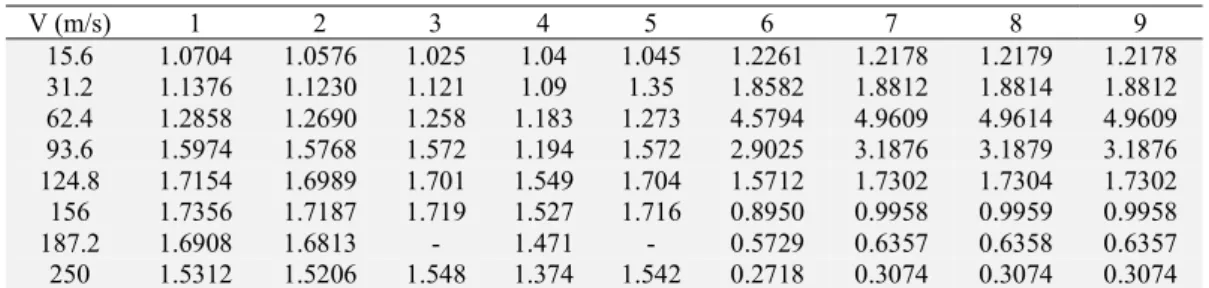
. In Table 3, dynamic amplification factors (DAF), defined as the ratio of maximum dynamic displace-ment to maximum static displacedisplace-ment, are compared with numerical, analytical and experidisplace-mental results using different theories available in the literature. For the Timoshenko beam (column 3) the results obtained with the present method appear to be close to the results of the analytical solution (Meirovitch, 1967) and the first order shear deformation theory (FSDT) (Michaltsos, 2002) . In addition, the current study and moving mass studies in the literature have been compared to show differences between moving mass and moving load assumptions, and the results of (Sharbati and Szyszkowski, 2011; Wu, 2005) and the present study are very close for moving mass assumption. However, unlike the moving load (motion force) approach which neglects the effects of mass inertia, the DAF has increased significantly at some high speeds, but at very low speeds, all results are very close.

Table 3: Dynamic amplification factors (DAF) versus velocity

V (m/s) 1 2 3 4 5 6 7 8 9

15.6 1.0704 1.0576 1.025 1.04 1.045 1.2261 1.2178 1.2179 1.2178

31.2 1.1376 1.1230 1.121 1.09 1.35 1.8582 1.8812 1.8814 1.8812

62.4 1.2858 1.2690 1.258 1.183 1.273 4.5794 4.9609 4.9614 4.9609

93.6 1.5974 1.5768 1.572 1.194 1.572 2.9025 3.1876 3.1879 3.1876

124.8 1.7154 1.6989 1.701 1.549 1.704 1.5712 1.7302 1.7304 1.7302

156 1.7356 1.7187 1.719 1.527 1.716 0.8950 0.9958 0.9959 0.9958

187.2 1.6908 1.6813 - 1.471 - 0.5729 0.6357 0.6358 0.6357

250 1.5312 1.5206 1.548 1.374 1.542 0.2718 0.3074 0.3074 0.3074

(1) Present moving load (TBT), (2) Present moving load (EBT), (3) Moving load, analytical from (Meirovitch, 1967), (4) Moving load, third order shear deformation theory (TSDT) from (Mohebpour et al., 2011), (5) Moving load (FSDT) from (Michaltsos, 2002), (6) Present moving mass (TBT), (7) Present moving mass (EBT), (8) Moving mass (EBT) from (Sharbati and Szyszkowski, 2011), (9) moving mass (EBT) from (Wu, 2005).

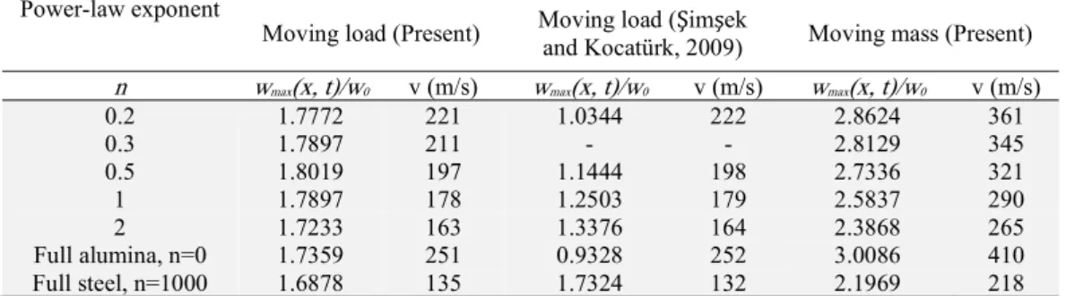
Example 2: let us consider the following FGM beam investigated by (Nguyen et al., 2013) and (_Şim_şek and Kocatürk, 2009), whose properties are shown in Table 4. Here, beam length L = 20 m, height h = 0.9 m, width 0.4 m and power law-exponent n = 0.2, 0.3, 0.5, 1, 2, 0, 1000. The calculated physical properties of the beam based on the power law-law-exponent are given in Table 5. It is assumed here that the beam is full steel on the base surface and full Al2O3 (99.9%) on the top surface. In columns 2 and 3, the effective Young's modulus’s and densities are given according to power-law exponent. In column 4 the term _Φ gives the relative significance of the shear deformations to the bending deformations, by setting _Φ = 0 for neglecting shear deformation, displacement functions Eq. (A.3) are exact for beam element of EBT. The loading is 100 kN, and the corresponding moving mass, mp in column 7 while mass of the beam mb is given in 6.

Table 4. Material properties of FGM components.

Properties Unit Steel Alumina (Al2O3)

E GPa 210 390

ρ kg/m3

7800 3960

(9)

Table 5. Material and physical properties of FGM beam based on power law exponent.

Power-law exponent n Ez(GPa) ρz (kg/m3) Φ z0(m) mb (kg) mp (kg) mpg

(kN)

0.2 360 4600 0.0793 0.017 33120 10193.7 100

0.3 348 4846 0.0793 0.0233 34892 10193.7 100

0.5 330 5240 0.0796 0.0327 37728 10193.7 100

1 300 5880 0.0811 0.045 42336 10193.7 100

2 270 6520 0.0832 0.05 46944 10193.7 100

Full alumina, n=0 390 3960 0.0797 0 28512 10193.7 100

Full steel, n=1000 213 7796 0.0861 0.0004 56132 10193.7 100

Dynamic amplification factors (DAFs) of the maximum midpoint displacements versus velocity of the mass for dif-ferent power-law exponents considering moving load and moving mass assumptions, are given in Figure 5. Where DAF Max (w(L/2, t))/ w0 is the ratio of the maximum displacement occurring at midpoint of the beam to the static displacement

occurring when the mass is statically at the midpoint of the beam, where w0 =FL3/48EzIz.

Figure 5. Dynamic amplification factors versus velocity of the mass for different power-law exponents considering moving load and moving mass assumptions.

In Table 6, the maximum DAFs and corresponding mass velocities are given in the assumption of moving mass and moving load. There are small differences in DAFs compared to the given in (_Şim_şek and Kocatürk, 2009) even if the corresponding velocities are the same or very close. These small differences are due to the same ratio of Poisson’s of alumina and steel, which is not clarified in (Şimşek and Kocatürk, 2009) and but they are accepted as the same in (Şimşek and Al-shujairi, 2017). The Poisson ratio of the alumina is v = 0.23 and it is 0.30 for the steel. Furthermore, the static deformation must be calculated considering the FGM beam, not the normal beam. Because, as seen in Table 5, the effec-tive-Young’s modulus, effective density, and beam mass vary according to the power-law exponent. This change affects both static and dynamic displacements. The other differences are the inclusions of axial coupling and rotary inertia. In this study, in addition to the shear effect, in the TBT (Timoshenko beam theory), the effects of the rotary inertia and axial coupling are fully applied. No effect has been neglected in this study, with the aim of setting up a basic reference to the future literature studies and researchers without neglecting the full effects.

Table 6. Maximum normalized deflections at the midpoint of the beam and corresponding velocities

Power-law exponent

Moving load (Present) Moving load (_{and Kocatürk, 2009)}Şimşek Moving mass (Present)

n wmax(x, t)/w0 v (m/s) wmax(x, t)/w0 v (m/s) wmax(x, t)/w0 v (m/s)

0.2 1.7772 221 1.0344 222 2.8624 361

0.3 1.7897 211 - - 2.8129 345

0.5 1.8019 197 1.1444 198 2.7336 321

1 1.7897 178 1.2503 179 2.5837 290

2 1.7233 163 1.3376 164 2.3868 265

Full alumina, n=0 1.7359 251 0.9328 252 3.0086 410

(10)

As can be seen from Fig. 5, the acceptance of moving mass leads to displacements which are twice as high as the moving load assumption. At small velocities below 25 m / s, both admissions yield close results. At high speeds, calculation of actual displacements with moving load assumption may give misleading results. As can be seen in Eqs. (A.6), the components of k vary linearly with the mass of the load while vary in proportion to the square of the velocity. At the same time, if the Coriolis effect is involved in the calculation, the components of the matrix c change linearly with both mass and velocity; and the effect of inertia is accounted for, the components matrix m vary depending on the mass. This negli-gence can be made at low speeds but must not be neglected at high and very high speeds.

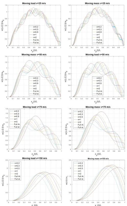
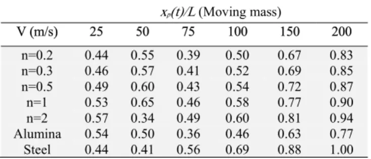
Nowadays, especially in the case of high-speed train transport, the speed of transport vehicles has reached 500 km/h, as is the case of the Japanese bullet train. For moving load and moving mass assumptions; to compare the effects of low and very high speed, Fig. 6 shows the results obtained at velocities of v = 25, 50, 75, 100, 150 and 200 m / s. In tables 7 to 10, the normalized maximum displacement and corresponding mass positions in these graphs are presented.

Table 7. Relative mass position of max. mid-point displacement xp(t)/L (Moving load)

V (m/s) 25 50 75 100 150 200

n=0.2 0.53 0.49 0.35 0.44 0.59 0.72

n=0.3 0.55 0.51 0.36 0.46 0.61 0.73

n=0.5 0.44 0.54 0.39 0.48 0.64 0.77

n=1 0.48 0.59 0.42 0.51 0.68 0.82

n=2 0.52 0.64 0.45 0.55 0.72 0.87

Alumina 0.47 0.44 0.63 0.40 0.54 0.66

(11)

(12)

Table 8. Normalized max. mid-point displacement.

w(L/2,t)/w0 (Moving load)

V (m/s) 25 50 75 100 150 200

n=0.2 1.10 1.19 1.14 1.39 1.68 1.77

n=0.3 1.10 1.21 1.19 1.44 1.72 1.79

n=0.5 1.10 1.22 1.26 1.51 1.76 1.80

n=1 1.13 1.19 1.34 1.58 1.77 1.78

n=2 1.10 1.10 1.36 1.57 1.72 1.69

Alumina 1.06 1.12 1.12 1.25 1.57 1.70

Steel 1.05 1.16 1.48 1.64 1.68 1.56

Table 9. Relative mass position of max. mid-point displacement xp(t)/L (Moving mass)

V (m/s) 25 50 75 100 150 200

n=0.2 0.44 0.55 0.39 0.50 0.67 0.83

n=0.3 0.46 0.57 0.41 0.52 0.69 0.85

n=0.5 0.49 0.60 0.43 0.54 0.72 0.87

n=1 0.53 0.65 0.46 0.58 0.77 0.90

n=2 0.57 0.34 0.49 0.60 0.81 0.94

Alumina 0.54 0.50 0.36 0.46 0.63 0.77

Steel 0.44 0.41 0.56 0.69 0.88 1.00

Table 10. Normalized max. mid-point displacement

w(L/2,t)/w0(Moving mass)

V (m/s) 25 50 75 100 150 200

n=0.2 1.09 1.22 1.29 1.66 2.11 2.36

n=0.3 1.12 1.22 1.35 1.71 2.15 2.37

n=0.5 1.15 1.20 1.43 1.78 2.20 2.37

n=1 1.14 1.12 1.53 1.85 2.20 2.32

n=2 1.08 1.10 1.55 1.84 2.11 2.21

Alumina 1.07 1.19 1.14 1.50 1.99 2.30

Steel 1.10 1.26 1.67 1.90 2.06 2.17

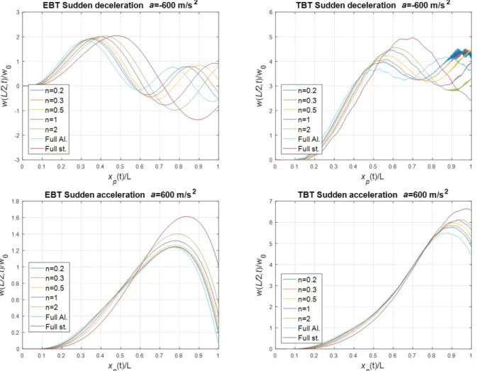
3.1 Effect of the Sudden Acceleration and Deceleration

The effects of sudden acceleration on systems such as missile launchers and bridges are worth examining today as they may be in the case of sudden accelerations of missiles and projectiles or sudden braking of high-speed vehicles. To examine this effect and analyse the interaction of the beam with the mass, the results of sudden acceleration and decelera-tion situadecelera-tions are given in the following secdecelera-tion. The same constant acceleradecelera-tion and deceleradecelera-tion rate of 600 m/s2_are

considered where the velocity of the mass is increased from zero to 154.86 m/s and decreased from this velocity to zero. In the case of acceleration, the mass is at the left end of the beam and the velocity is zero. In the case of braking, the velocity of the mass is zero at the right end of the beam.

(13)

EBT can be applied instead of TBT as the results will be close to each other. We have chosen the example of high accel-eration with the aim of revealing the difference between these two theories. In the case of accelaccel-eration and decelaccel-eration, considering the relative position of the mass on the beam, the contact point xp of the mass varies with a quadratic function

of time while the velocity of the mass varies linearly, therefore, according to the relative position, it is expected that the displacement graphs of both situations will be very different. at rapid acceleration, the mass starts to accelerate from the left end of the beam, and before it reaches a quantity that will magnify the beam vibrations, the mass travels a great deal over the beam. Only after the mass passes the midpoint of the beam, the vibrational amplitudes grow. In the case of deceleration, the amplitudes increase earlier as the initial velocity and acceleration are higher. Another point is that the early excited beam has already begun to vibrate. The vibration amplitude tends to decrease with a fluctuation although the velocity of the mass rapidly decays over time. The decrease in amplitude is not as fast as the decrease in mass velocity. These events can be observed in both EBT and TBT models.

. These events can be observed in both EBT and TBT models.

(14)

Figure 8. Axial normalized mid-point displacements of the FGM compounds for sudden acceleration and deceleration using EBT and TBT.

4 CONCLUSIONS

In this study, a realistic model of a FGM Timoshenko beam under the influence of accelerated mass is established. The inertia effect of moving masses which are not adequately addressed in the literature studies for FGM beams is widely presented for different speeds and accelerations. It is understood that the dynamic behaviour of the beam is not overly affected by inertia effects at low and constant load speeds, as indicated in the literature for low speed civil engineering applications. However, at high speeds and in the case of acceleration or deceleration, it has been observed that the dynamic behaviour of the FGM beam changes significantly due to effect of the mass of the load. In some cases, the DAF increased by a factor of 2 due to the natural frequency change in the beam under the influence of the moving mass. In the analyses made, it was observed that the fundamental frequency changed by 50% (figures 5 and 6) when the mass of the moving load was equal to the mass of the beam. Thus, the decrease in fundamental frequency will reduce the speed parameter of the load. The speed parameter is the ratio of the influence frequency (ω=πv/L) of the moving mass to the actual funda-mental frequency of the beam. The speed parameter of the fundafunda-mental frequency is defined as the ratio of _ω/_ω1, and the maximum response occurs when this ratio is equal to 1. It was also emphasized that design and calculation should be done considering the frequency variation in FGM applications where the mass and velocity of the load is high, and the speed of motion is not constant.

Modelling of the FGM beam with a moving mass have been extensively studied in the assumptions of TBT, EBT, moving mass and moving load at constant and variable moving speeds of the mass, and results of the analysis have been given in detail. The effects of sudden acceleration / deceleration cases on transverse and axial vibration of the FGM beam were also presented.

References

(15)

Chakraborty, A., Gopalakrishnan, S., Reddy, J.N., 2003. A new beam finite element for the analysis of functionally graded materials. Int. J. Mech. Sci. 45, 519–539. doi:10.1016/S0020-7403(03)00058-4

Cifuentes, A.O., 1989. Dynamic response of a beam excited by a moving mass. Finite Elem. Anal. Des. 5, 237–246. doi:10.1016/0168-874X(89)90046-2

Ebrahimi, F., Shaghaghi, G.R., Boreiry, M., 2016. A Semi-Analytical Evaluation of Surface and Nonlocal Effects on Buckling and Vibrational Characteristics of Nanotubes with Various Boundary Conditions. Int. J. Struct. Stab. Dyn. 16, 1–20.

Eltaher, M.A., Alshorbagy, A.E., Mahmoud, F.F., 2013. Determination of neutral axis position and its effect on natural frequencies of functionally graded macro/nanobeams. Compos. Struct. 99, 193–201. doi:10.1016/J.COMP-STRUCT.2012.11.039

Esen, _İ., 2013. A new finite element for transverse vibration of rectangular thin plates under a moving mass. Finite Elem. Anal. Des. 66, 26–35. doi:10.1016/j.finel.2012.11.005

Jafari-Talookolaei, R.-A., Ebrahimzade, N., Rashidi-Juybari, S., Teimoori, K., 2018. Bending and vibration analysis of delaminated Bernoulli-Euler microbeams using the modified couple stress. Sci. Iran. 25, 675–688. doi:10.24200/sci.2017.4252

Kadivar, M.H., Mohebpour, S.R., 1998. Finite element dynamic analysis of unsymmetric composite laminated beams with shear effect and rotary inertia under the action of moving loads. Finite Elem. Anal. Des. 29, 259–273. doi:10.1016/S0168-874X(98)00024-9

Kang, Y.A., Li, X., 2010. Large deflection of a non-linear cantilever functionally graded beam. J Reinf Plast Compos 29, 1761–1774.

Khan, A.A., Alam, M.N., ur Rahman, N., Wajid, M., 2016. Finite element modelling for static and free vibration response of functionally graded beam. Lat. Am. J. Solids Struct. 13, 690–714. doi:10.1590/1679-78252159

Kim, N.-I., Lee, J., 2014. Exact solutions for stability and free vibration of thin-walled Timoshenko laminated beams under variable forces. Arch. Appl. Mech. 84, 1785–1809. doi:10.1007/s00419-014-0886-2

Kosmatka, J.B., 1995. An improved two-node finite element for stability and natural frequencies of axial-loaded Timo-shenko beams. Comput. Struct. 57, 141–149. doi:10.1016/0045-7949(94)00595-T

Lien, T.V., Duc, N.T., Khiem, N.T., 2017. Free vibration analysis of multiple cracked functionally graded Timoshenko beams. Lat. Am. J. Solids Struct. 14, 1752–1766. doi:10.1590/1679-78253693

Mashat, D.S., Carrera, E., Zenkour, A.M., Al Khateeb, S.A., Filippi, M., 2014. Free vibration of FGM layered beams by various theories and finite elements. Compos. Part B Eng. 59, 269–278. doi:10.1016/J.COMPOSITESB.2013.12.008 Masoodi, A.R., Moghaddam, S.H., 2015. Nonlinear dynamic analysis and natural frequencies of gabled frame having flexible restraints and connections. KSCE J. Civ. Eng. 19, 1819–1824. doi:10.1007/s12205-015-0285-4

Meirovitch, L., 1967. Analytical methods in vibrations. The Macmillan Company, New York.

Michaltsos, G., 2002. Dynamic behaviour of a single-span beam subjected to loads moving with variable speeds. J. Sound Vib. 258, 359–372. doi:10.1006/jsvi.5141

Mohebpour, S.R., Malekzadeh, P., Ahmadzadeh, A.A., 2011. Dynamic analysis of laminated composite plates subjected to a moving oscillator by FEM. Compos. Struct. 93, 1574–1583. doi:10.1016/J.COMPSTRUCT.2011.01.003

(16)

of material properties. Eng. Struct. 32, 1631–1640. doi:10.1016/J.ENGSTRUCT.2010.02.010

Nguyen, D.K., Gan, B.S., Le, T.H., 2013. Dynamic Response of Non-Uniform Functionally Graded Beams Subjected to a Variable Speed Moving Load. J. Comput. Sci. Technol. 7, 12–27. doi:10.1299/jcst.7.12

Nguyen, T.-K., Nguyen, B.-D., 2015. A new higher-order shear deformation theory for static, buckling and free vibration analysis of functionally graded sandwich beams. J. Sandw. Struct. Mater. 17, 613–631. doi:10.1177/1099636215589237 Rajabi, K., Kargarnovin, M.H., Gharini, M., 2013. Dynamic analysis of a functionally graded simply supported Euler– Bernoulli beam subjected to a moving oscillator. Acta Mech. 224, 425–446. doi:10.1007/s00707-012-0769-y

Rezaiee-Pajand, M., Masoodi, A.R., 2016. Exact natural frequencies and buckling load of functionally graded material tapered beam-columns considering semi-rigid connections. J. Vib. Control 24, 1787–1808. doi:10.1177/1077546316668932

Rezaiee-Pajand, M., Mokhtari, M., Masoodi, A.R., 2018. Stability and free vibration analysis of tapered sandwich columns with functionally graded core and flexible connections. CEAS Aeronaut. J. 1–20. doi:10.1007/s13272-018-0311-6 Rezaiee-Pajand, M., Rajabzadeh-Safaei, N., 2018. Nonlocal static analysis of a functionally graded material curved nano-beam. Mech. Adv. Mater. Struct. 25, 539–547. doi:10.1080/15376494.2017.1285463

Sharbati, E., Szyszkowski, W., 2011. A new FEM approach for analysis of beams with relative movements of masses. Finite Elem. Anal. Des. 47, 1047–1057. doi:10.1016/J.FINEL.2011.03.020

Şim_şek, M., Al-shujairi, M., 2017. Static, free and forced vibration of functionally graded (FG) sandwich beams excited by two successive moving harmonic loads. Compos. Part B Eng. 108, 18–34. doi:10.1016/J.COMPOSITESB.2016.09.098 Şim_şek, M., Kocatürk, T., 2009. Free and forced vibration of a functionally graded beam subjected to a concentrated moving harmonic load. Compos. Struct. 90, 465–473. doi:10.1016/j.compstruct.2009.04.024

Sina, S.A., Navazi, H.M., Haddadpour, H., 2009. An analytical method for free vibration analysis of functionally graded beams. Mater. Des. 30, 741–747. doi:10.1016/J.MATDES.2008.05.015

Taati, E., 2018. On buckling and post-buckling behavior of functionally graded micro-beams in thermal environment. Int. J. Eng. Sci. 128, 63–78. doi:10.1016/J.IJENGSCI.2018.03.010

Taeprasartsit, S., 2013. Nonlinear free vibration of thin functionally graded beams using the finite element method. J. Vib. Control 21, 29–46. doi:10.1177/1077546313484506

Wang, Y., 2009. The transient dynamics of a moving accelerating / decelerating mass traveling on a periodic-array non-homogeneous composite beam. Eur. J. Mech. A/Solids 28, 827–840. doi:10.1016/j.euromechsol.2009.03.005

Wu, J.-J., 2005. Dynamic analysis of an inclined beam due to moving loads. J. Sound Vib. 288, 107–131. doi:10.1016/j.jsv.2004.12.020

Yokoyama, T., 1996. Vibration analysis of Timoshenko beam-columns on two-parameter elastic foundations. Comput. Struct. 61, 995–1007. doi:10.1016/0045-7949(96)00107-1

Yoshida, D.M., Weaver, W., 1971. Finite-element analysis of beams and plates with moving loads. Int. Assoc. Bridg. Struct. Eng. 31, 179–195.

(17)

Appendix A

The vectors of shape functions for u, w and θ, respectively in Eq. (14) are in the form

 

1 2 3 4 5 6

T

u u u u u u u

T

w w w w w

T                                  _ _    _ _    _ _ (A.1) with

















2 2

1 2 3

2 2

4 5 6

2

12 11 2 22 33 12 11 33

6

1 , , 3 (4 ) (1 )

(1 ) (1 )

6

, , 3 (2 ) ,

(1 ) (1 )

12( )

, / , ; / ; / ( )

u u u

l

l x

D D D D D D D

l l                                                              (A.2)





3 2

1 4 2

3 2 3 3 2 5 3 2 6 1

0, 2 3 1 ,

1

2 1 ,

1 2 2

1

2 3 ,

1

1 2 2

w w w

w w w l l                        __      __    _ __ _ __       _  _ __  _ __ _    _     _     __    __    _ __ _   _   _  _ __  _   _   _ (A.3)









2 2

1 4 2 3

2 2

5 6

1 6 1

0, , 3 (4 ) 1 ,

1 1

1 6 1

, 3 2

1 1 l l                            __  __  __      __           __  __  __   __     (A.4)

Derivation of Eq. (25)

Eq. (24) is evaluated using nodal displacement equations in Eq. (14) using



u_and



w_{including shear deformation} effects but omitting rotatory coupling with axial motions. In such a case, the external force equations for the contact point of the mass are:

d

d d

1 4

2

2 3 5 6

( ( , )),

0 0 0 0 ( 1, 4)

( ( , ) 2 ( , ) ( , ) ( , )) ,

0 0

2 0 0

ix ui p p

T

xi ui p p ui u u

zi wi p p p p p

T

zi p wi w w w w

T

p wi w w w w

p w

f m a u x t

f m a m i

f m g w x t vw x t v w x t aw x t

f m vm m                        __ __   _ _ _   __     __    __ __  _ _ _ _   __ __       d