Abstract
In this paper, a new modified finite element method that can be used in the analysis of transverse and lateral vibrations of the thin beams under a point mass moving with a variable acceleration and constant jerk is presented. Jerk is the change in acceleration over time. In this method, the classical finite element of the beam is mod-ified by the inclusion of the inertial effects of the moving mass. This modification is made using the relations between nodal forces and nodal deflections and shape functions of six DOF beam element. The mass, stiffness, and damping matrices of the modified finite element are determined by forces caused by the corresponding transverse and lateral accelerations and jerks, and transverse Coriolis and centrip-etal accelerations and jerks, respectively. This method was first ap-plied on a simply supported beam plate to provide a comparison with the previous studies in literature, and it was proved that the results were within acceptable limits. Secondly, it was applied on a CNC type box-framed beam to analyse the dynamic response of the beam in terms of variable acceleration and jerk as well as constant velocity and mass ratios.
Keywords
Finite element, beam vibrations, accelerating mass, jerk.
A Modified FEM for Transverse and Lateral Vibration Analysis
of Thin Beams Under a Mass Moving with a Variable Acceleration
1 INTRODUCTION
Dynamic behaviour of mechanical and structural systems with moving masses is a very important engineering problem. In the design of the running systems under very high-speed masses and with a very little working tolerance such as high speed precision metal processing, high-speed rail transpor-tation, robotics applications in microchip production, high-speed projectile firing from a barrel, high– speed rocket launching systems, and etc., some new engineering problems arise together with speed increase. In such systems, the pre-engineering analysis must be accurate in order to prevent possible accidents and failures in the application. For example, the design and development studies of a missile and high-speed rail systems that cost millions of dollars should not only depend on experimental
Ismail Esen
Department of Mechanical Engineering, Karabük University, Karabük, Turkey [email protected]
http://dx.doi.org/10.1590/1679-78253180
studies. When an accident is happened, no one retrieve the situation in an experimental trial. In this case, realistic modelling and analysis is vital for such systems. The computation methods given in literature are commonly for low speeds and simple cases where the motion at variable speeds, accel-eration and inertia effect of mass are neglected. In this study, a more realistic method of modelling and analysis of such systems is provided without neglecting the damping, inertia effects of the mass in motion, effect of a variable speed, effect of a variable acceleration, and effect of a constant jerk. Due to the variety of its applications, the moving load problem has been widely studied in literature by many researchers. For example, (Gerdemeli et al. 2011, Kahya 2012, Sharbati and Szyszkowski 2011, and Esen 2013) have studied the subject for a constant velocity of a moving mass. An analytical solution of the effects of moving load motion for Timoshenko beams has been provided by Lee 1996. Considering the effect of a variable velocity load on structures (Michaltsos 2002, Wang 2009, Esen 2011, and Dyniewicz and Bajer 2012 have studied the dynamic behaviour of beams under accelerated masses. Inertia effects of the moving mass continue to be a point of interest for bridge dynamics, railroad design, and other high-velocity delicate motion processes and some others (Michaltsos et al. 1996, Michaltsos and Kounadis 2001, and Dehestani et al. 2009) have studied and proposed some simplified analytical solutions of the inertial effects of moving masses. Wu 2005 has studied the vertical and horizontal displacements of an inclined simply supported beam under moving loads for the effects of the velocity and the mass of a moving-load including the Coriolis and centrifugal forces and incli-nation angle of the beam. Omolofe 2013 has presented a procedure involving spectral Galerkin and integral transformation methods for the problem of the dynamic deflections of beam structure resting on bi-parametric elastic subgrade and subjected to travelling loads. Oni and Awodola 2010, and Awodola 2014 have studied the dynamic response of an elastically supported non-prismatic Bernoulli-Euler beam and the flexural motions of elastically supported rectangular plates carrying moving masses and resting on variable Winkler elastic foundations. For the application of the moving load problem in defence field, a finite element model of a high-speed projectile and barrel interaction has provided by Esen and Koç 2015a, 2015b. Another Finite element application of the moving load on plate dynamics can be found in Esen 2015. The dynamics of a railcar bogie when moving over a flexible bridge has been studied by Mizrak and Esen 2015 as an application in high-speed rail trans-portation.
of the work performed. Therefore, the velocity, acceleration, and jerk of the mass are vital in terms of the accuracy of such mechanical engineering applications. The main purpose of this study is exam-ining the issue in this perspective.
2 MATHEMATICAL MODELLING
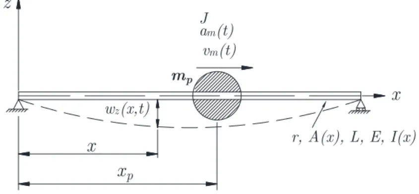
In Figure 1, a simply supported Euler-Bernoulli beam with a lumped mass mp which is travelling on
the beam from the left end to the right end with a variable velocity vm(t), a variable acceleration am (t) and a constant jerk J, is given.
In the formulation the following assumptions will be adopted (Fig. 1)
The mass inertia is considered.
The mass is always in contact with the beam.
The beam is thin and small displacements in the beam are occurred according to thin beam theory.
Figure 1: A simply supported beam and a moving mass system.
The beam can be of variable thickness but the material properties are constant trough length of the beam.
In vibration, the longitudinal and flexural motions are independent of each other but the axial force due to the acceleration of the mass affects the flexural displacements.
The trajectory of the mass is defined by time-dependent xp(t)
Based on the above assumptions, the motion equation of the beam due to the effect of the mass located at the time-dependent point xpon the beam is provided by Eq. (1) Fryba 1999:
4 2 2
4 2 2
2
2
( , ) ( , ) ( , ) ( , )
( ) ( , ) ( ) ( , ),
d ( , )
( , ) ( ( )) ( ( )),
d
z z z z
z p
p p p p
w x t w x t w x t w x t
EI x N x t A x F x t
t
x x t
w x t
F x t m g x x t m x x t
t
r s
d d
¶ ¶ ¶ 
- + + =
¶ ¶ 
æ ö÷
ç ÷
ç ÷
= - - çç ÷÷
-ç ÷÷
çè ø
(1) vm(t)
mp
r, A(x), L, E, I(x)
x
z
x
px
wz(x,t)
The left hand side of Eq. (1) represents the resisting internal stiffness, inertia and damping forces due to the external forces on the right side with the parameters that: N(x,t) represents the time dependent axial load due to the acceleration of the moving mass; ρ represents the density, A(x)
represents the none uniform cross-sectional area, σ represents equivalent viscous damping coefficient,
E represents the Young’s modulus of elasticity, I(x) represents the area moment of inertia, x repre-sents the central coordinate of the beam, t represents time, wz(x, t) represents the vertical
displace-ment of the beam, mp represents the mass of the load, m g xp d( -xp(t)) represents the force applied
to the unit length of the beam by the moving mass, gand δ represent gravitational acceleration and
the Dirac delta function, respectively, and d2w(x
p,t)/dt2 represents the acceleration of the beam at the
contact point of lumped mass.
The initial and boundary conditions of the beam are:
2 2
2 2
( 0, ) ( , ) 0,
( 0, ) ( , )
0
w x t w x L t w x t w x L t
x x
= = = =
¶ = = ¶ = =
¶ 
(2)
In order to determine time dependent displacements of the beam, a rough analytical solution of the motion Eq. (1) shown above, can be obtained through simplifications that ignore the effects of inertia and damping; and accepting that the cross-section area is uniform and the mass moves with a constant velocity. For simplified cases, omitting geometric and dynamic nonlinearities such moving load problems have been extensively studied in the literature by numerous researchers. When the mass moves with a constant jerk on the beam, the exact solution of the motion equation using ana-lytical methods will be very difficult; and no study of constant jerky motion of a mass has been reported in literature, yet. This kind of motion problems are faced frequently in today’s engineering applications such as high-speed precision machining, precision grinding of hard cutting tools, some robotic applications of precision surgical robots and precision robots used in microchip production; where vibration of the linear run-ways are vital for the accuracy of the work done. For an exact or an admissible solution in the engineering sense, there are needs of some new methods that represent mass motion with all effects including jerk. This paper presents a solution method representing the mass as a time dependent finite element and combining this finite element with the classical finite elements of the beam. This method includes both inertial and damping effects and gives a solution for both transverse and longitudinal vibrations of the beam. From this perspective, the proposed FEM combined method can be very useful for design and control engineers if they pay attention to the requirements of modelling as described below.
2.1 Modified Mass, Damping and Stiffness Matrices of the Beam Element
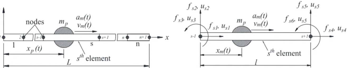
Figure 2 displays mesh discretion of a thin beam under a lumped moving mass and the beam element s on which the mass mp applies, at time t. The beam element s has three equivalent nodal forces and
displacements at each nodal point. The time-dependent global position of the moving mass in the span is xp (t), while local position on the length of the element s is xm (t). The beam has n elements
Figure 2: Finite element model of a thin beam with a lumped moving mass and equivalent nodal forces and displacements of the beam element s.
For any time t, the effective transverse (z) force at coordinate x, due to the interaction between the moving mass and the beam which is vibrating and deflected, can be determined as follows using he principle of D’Alembert :
(
)
2 2
2 3
0 0 0
2 0 0
2
0 2
d ( , )
( , ) ,
d
1 1
,
2 6
d 1
,
d 2
d d
, ,
d d
z p
z p p
p
p m
p m
m
w x t
f x t m g x x
t
x x v t a t Jt
x
v v a t Jt
t
x a
a a Jt J
t t
d
é ù
ê ú
= ê - ú
-ê ú
ë û
= + + +
= = + +
= = + =
(3)
For the linear motion of a particle object, the instantaneous acceleration is derived using the constant jerk of the motion and integrating it with respect to time for an increment of time Δtfrom t-Δtto t, as given below:
t t t
a =a-D + DJ t (4)
Considering continuous contact between the mass and beam, when the mass moves on the beam with a variable acceleration and a constant jerk, the instantaneous flexural acceleration of the contact point of the mass can also be determined using the definite integration of the differential acceleration and jerk equation over a small time increment Δt, in the same way as Eq. (4). In such case, the effective transverse force equation will be rearranged as follows:
(
)
2 3
2 3
d ( , ) d ( , )
( , ) ,
d d
t
t t
z p z p
t
z p p
w x t w x t
f x t m g t x x
t t d
-D
é æ öù
ê çç ÷÷ú
ê ç ÷ú
= ê -ç + D ÷÷ú
-ç ÷
ê çè ÷øú
ê ú
ë û
(5)
When the necessary total differentiations of deflection function wz (x, t) with respect to the time
dependent contact point xp of the moving mass at time t, are determined and after making some
mathematical arrangements, Eq.(5) becomes:
sth element l
1 s n
z
x
xp (t) xm(t)
L
1 2 s-1 s+1 n n+1 s-1 s+1
sth element
nodes
fs4, us4
mp mp
fs5, us5
fs6, us5
fs2, us2
fs3, us3
fs1, us1
vm(t)
am(t)
vm(t)
(
)
(
)
(
)
2
3 2
( , ) 2
3 3 3 ,
t t
t
z p p z z z z
t
p z z z z z z z p
f x t m g m w vw v w aw
m v w v w vaw vw aw Jw w t xd x
-D
-D
¢ ¢¢ ¢
= - + + + +
¢¢¢ ¢¢ ¢¢ ¢ ¢ ¢
+ + + + + + + D
-
(6)
where the acceleration and jerk are
2 2 2 3 3 2 3 2 3 2 3
d ( , )
2 ,
d
d ( , )
3 3 3 ,
d
d d d
; ;
d d d
p p p
z p
z z z z
z
z z z z z z z
x x x x x x
w x t
w vw v w aw
t w x t
w v w v w va w v w a Jw w t
x x x
v a J
t = t = t =
¢ ¢¢ ¢ = + + + ¢¢¢ ¢¢ ¢¢ ¢ ¢ ¢ = + + + + + + = = =
(7)
where “ ′ ” and “ · ” are, respectively, spatial and time derivatives of deflection. Derivation of the
acceleration and jerk terms are given in Appendix A. The terms
(
2)
2 t t
z z z z
w + vw¢+v w¢¢+aw¢ -D in Eq.
(6), represent the inertia, the Coriolis and the centripetal acceleration components at time t-Δt, while
(
3 2)
3 3 3 t
z z z z z z z
v w¢¢¢+ v w¢¢+ vaw¢¢+ vw¢+aw¢+Jw¢+w represent jerks for above mentioned acceleration
com-ponents of the interaction of the mass and beam at time t. Wherewz is inertia; 2vwz¢ is Coriolis,
2
z z
v w¢¢+aw¢ is centripetal acceleration components, while wz +3vwz¢ is inertia,3 2
z z
v w¢¢+aw¢ is Coriolis
and 3 3
z z z
v w¢¢¢+ vaw¢¢+Jw¢ is Centripetal jerks of the accelerations respectively. In vibration, the inertia
jerk of the beam can be approximated using the average acceleration method proposed by Newmark in the Beta method of integration with in the assumptions of the method. In this case the jerk of the beam is:
1
,
t t
t t
z z z
w w w
t
-D
é ù
= êë - úû
D
(8)
When the beam is in vibration, the longitudinal (x) force component, between the moving mass and the beam, induced by the vibration and curvature of the deflected beam is
(
)
2
2
d ( , )
( , ) ( ) ( ),
d
x p
t t t t
x p p p p x p
w x t
f x t m a x x m a J t m w x x
t d d
-D
æ ö÷
ç ÷
ç
= çç - ÷÷ - = - + D +
-÷÷
çè ø (9)
The equivalent nodal forces of the beam element s under a lumped moving mass that has a variable acceleration and a constant jerk are:
(
)
( )
(
2)
3 2
( 1, 4),
2
1
3 3 3
( 2, 3, 5, 6),
t t t
t t t
si i p i p x
t t t
si i p z z z z
t t
t
i p z z z z z z z z
i p
f m a J t m w i
f m w vw v w aw
m w v w v w va w v w a Jw w w t
t m g i
f f f f f -D -D -D -D
= - + D + =
¢ ¢¢ ¢
= + + +
æ é ùö÷
ç ¢¢¢ ¢¢ ¢¢ ¢ ¢ ¢ ÷
+ ççç + + + + + + êë - úû÷÷ D
D
è ø
- =
Where, ϕi (i=1- 6) are shape functions of the beam element given by Clough and Penzien, 2003;
these are cubic Hermitian polynomials that are expressed as
2 3 2
1 2 3
2 3 2
4 5 6
1 , 1 3 2 , 1 ,
, 3 2 , 1 ,
x x x x
x
l l l l
x x x x x
l l l l l
f f f
f f f
æ ö÷ æ ö÷ æ ö÷
ç ÷ ç ÷ ç ÷
= - = - ççç ÷÷ + ççç ÷÷ = ççç - ÷÷
è ø è ø è ø
æ ö÷ æ ö÷ æ ö÷
ç ÷ ç ÷ ç ÷
= = ççç ÷÷ - ççç ÷÷ = ççç - ÷÷
è ø è ø è ø
(11)
where l the length of s-th beam element.
The relation between shape functions and transverse and longitudinal displacements of the s-th beam element at position x and time t, is (Clough and Penzien, 2003):
1 1 4 4
2 2 3 3 5 5 6 6
( , ) ,
( , ) ,
x s s
z s s s s
w x t u u
w x t u u u u
f f
f f f f
= +
= + + + (12)
where usi (i = 1–6) are the displacements for the nodes of the s-th beam element on which the moving
mass mplocates at time t.
The property matrices of a beam element without any moving mass, in Fig. 2, having both transverse and longitudinal nodal forces and deflections, are derived from the usage of the principle of virtual works. Introducing the principle of virtual displacements, and applying unit displacements at the nodal points and then equating the work done by the external forces to the work done on the internal forces: WE = WI (Clough and Penzien, 2003) for a uniform beam segment using the
interpo-lation functions of Eq. (11), a stiffness equation can be obtained for the stiffness coefficients. For the mass coefficients, an elemental balance equation can be obtained using the relation between nodal accelerations and resisting inertial forces with the help of the same interpolation functions. In the special case of a beam element with uniformly distributed mass and under a mass moving with a variable acceleration over the beam element, the coefficients of modified mass, stiffness and equivalent damping matrices of the beam element s can be obtained by taking into account the contribution of inertial, Coriolis and centripetal forces due to the related accelerations and jerks (7) induced by the moving mass. In such a case, the total force balance equation for the beam element s is obtained in matrix form as below:
,
t t t t t t t
s s s
= + +
f m u c u k u (13a)
,
t t t t
t
-D -D
= + + D
t
w w
m m m m
(13b)
,,
t t t t
t
-D -D
= + + D
t
w w
c c c c
(13c)
,
t t t t t
G t
-D -D
= + + w + w D
k k k k k
(13d)
where m, c and k are, respectively, the modified mass, damping and stiffness matrices of the beam
element s that includes all the effects of the moving mass, while m, c and k are consistent mass,
and kG is the geometric stiffness matrix due to the axial force N(x,t). The matrices
w
m
andmw, cw
andcw, kw and kw are derived from the interaction of the moving mass and the beam element and
they represent the moving mass with a constant jerk. The components of these matrices vary depend-ing on the motion velocity, acceleration and jerk, and the position of the mass on the beam element. The coefficients of these matrices are obtained from the equivalent nodal force equation (10) of the beam element s. One can obtain these matrices using the relation between the nodal displacements and the deflection functions (12) with the interpolation functions (11), and then putting them in the nodal force equation (10). After obtaining the spatial and time derivatives of the deflection function, Eq. (10) is rearranged separately for acceleration and jerk in terms of nodal accelerations, nodal velocities and nodal displacements, thus these matrices are obtained, as given in Appendix B.
During the integration of motion equation of the overall system, the instantaneous values of these matrices are calculated at every time step Δt, an then added to the values of the matrices of the beam element s on which the moving mass locates at time t. Because, they are derived from the relation between nodal displacements and shape functions of the two-node beam element, the dimen-sions of these matrices are equal to the dimendimen-sions of the mass, damping, stiffness matrices of the beam element. Hence, the beam element has three displacements DOF at each end nodal point; the dimensions of these modification matrices will also be 6x6.
The consistent mass, equivalent damping and consistent stiffness matrices m, c, and k, of the
beam element s are calculated using their coefficients mij, cij, andkij, as given below
0
0 0
0 0
0
( ) ( ) ( ) ,( , 1, 2, 3, 4, 5, 6),
( ) ( ) ( ) ( ) ( ) ,( , 1, 4),
( ) ( ) ( ) ( ) ( ) ( ) ,( , 2, 3, 5, 6),
( ) ( ) ,( ,
l
ij i j
l l
ij i j i j
l l
ij i j i j
l
ij i j
m m x x x dx i j
c m x x x dx EA x x dx i j
c m x x x dx EI x x x dx i j
k EA x x dx i
f f
y f f t f f
y f f t f f
f f
= =
¢ ¢
= - =
¢¢ ¢¢
= + =
¢ ¢
=
-ò
ò
ò
ò
ò
ò
0
1, 4),
( ) ( ) ( ) ,( , 2, 3, 5, 6),
l
ij i j
j
k EI x f x f x dx i j =
¢¢ ¢¢
=
ò
=(14)
Where yand t are the coefficients for the equivalent viscous damping. They can be determined by using Rayleigh damping theory in which the coefficients of damping matrix is proportional to the combination of coefficients of the mass and stiffness matrices, as given by
(
)
(
)
2 2 2 2
,
2 2
, ,
ij ij ij
i j i j j i j j i i
j i j i
c ym tk
w w z w z w z w z w
y t
w w w w
= +
-
-= =
-
-(15)
where ζiandζjare the damping ratios of the structural system for any corresponding natural
In order to include the flexural effect of an axial load N(x,t) due to the acceleration of the mass, that is negative for positive acceleration and vice versa, the geometric stiffness matrix kG are obtained
with the following coefficients:
, 0
( , ) ( ) ( ) , ( , 2, 3, 5, 6),
l
Gi j i j
k =
ò
N x t f¢x f¢x dx i j = (16)where kGi j, are the coefficients of consistent geometric stiffness matrix and the Hermitian interpolation functions. Eqs. (11) are used in deriving the geometric stiffness coefficients.
In the time dependent elemental equation of motion of the beam element s, in Eq. (13a), the force ft
is as given below:
(
)
(
)
1 2 3 4 5 6
1 1
2 2
3 3
4 4
5 5
6 6
,
,
,
,
, , ,
T t
s s s s s s
t t
s p
s p
s p
t t
s p
s p
s p
f f f f f f
f m a J t
f m g
f m g
f m a J t
f m g
f m g
f f f
f f f -D
-D
é ù
= êë úû
= + D
= =
= + D
= =
f
(17)
The nodal acceleration, velocity, and displacement vectors, t, t, and t
s s s
u u u of the beam element
s are given by
1 2 3 4 5 6
1 2 3 4 5 6
1 2 3 4 5 6
,
,
,
T t
s s s s s s s
T t
s s s s s s s
T t
s s s s s s s
u u u u u u
u u u u u u
u u u u u u
é ù
= êë úû
é ù
= êë úû
é ù
= êë úû
u u u
(18)
2.2 Equation of Motion of the entire System
The equation of motion for the multiple degree of freedom damped structural system, shown in Fig. 2, is given by
,
+ + =
Mu Cu Ku F (19)
where M, C and K are, respectively, the overall mass, damping and stiffness matrices, while u, u
and u are respectively, the acceleration, velocity and displacement vectors. Besides, F is the overall
external force vector of the system at time t.
In general, such a structural system shown in Fig. 2, one can obtain overall mass M, stiffness K
andC matrices by assembling its element matrices and imposing given boundary conditions. If there
and centripetal forces, and jerks induced by moving mass. This is done by modifying only the ele-mental matrices of the beam element s on which the moving mass locates at time t, and keeping the elemental matrices of the other elements the same as original. The instantaneous overall force vector is also time-depended. The coefficients of overall force vector are equal to zero except the nodal forces of the beam element s. Thus, the instantaneous overall force vector of entire system becomes as below:
1 2 3 4 5 6
0 ... ... 0 ,
( 2, 3, 5, 6),
( ( ) ) ( 1, 4)
T
s s s s s s
s i p i
s i p i
f f f f f f
f m g i
f m a t t J t i
f
f
é ù
= êë úû
= =
= - D + D =
F
(20)
In evaluation of the matrices of the beam element s, for the instantaneous position of the mass, the term x in the Eq. (11) is replaced with xm (t). The instantaneous values of xm (t) and s can be
determined as follows:
( ) ( ) ( 1) ,
( )
(integer part of ) 1, (1 ),
m p
p
x t x t s l
x t
s s n
l
=
-= + = - (21)
2.3 Solution of Equation of Motion
If the added matrices ofmw,mw,kw, kw, kG and the equivalent force vector f are zero, the undamped
natural frequencies and vibration mode-shapes of the beam are obtained from homogenous solution of (19). In such a case, the Equation (19) reduces to
0,
+ =
Mu Ku (22)
The solution of (22) can be assumed as
, i t
ew =
u A (23a)
2 ei tw, w
=
-u A (23b)
Introducing the latter u and u into (22) gives
2
(K-w M)Ψei tw =0, (24)
This is a set of homogeneous equations, for which a nontrivial solution exists if
2
det(K-w M)=0, (25)
The above determinant equation is satisfied for a set of n values of frequency ω1, ω2,.., ωn. The
frequency ωi is called the i-th natural frequency. Substituting all the ωi into (24) yields the
For such a system, given in (19), one can obtain a solution by using a numerical integration method like Newmark’s method [5]. Using the Newmark integration method, equation (19) is transformed to equivalent stiffness and force equations. Thus, for the n-th time step at time tn (=tn-1+Δt):
0 1 ,
a a
= + +
K K M C (26)
0 1 2 1 3 1
1 1 4 1 5 1
( ) ( ) ( ) ( ) ( )
+ [ ( ) ( ) ( )].
n n n n n
n n n
t t a t a t a t
a t a t a t
- -
-- -
-é ù
= + êë + + úû
+ +
F F M u u u
C u u u
(27)
where u(tn-1), 1 (tn-)
u ,
1 (tn-)
u are, respectively, the initial conditions for the accelerations, velocities
and displacements of the structural system at time t = tn. Displacements at time tn
1
( )tn = - ( ),tn
u K F (28)
Accelerations and velocities at time tn
(
0 1)
2 1 3 1( )tn = a ( )tn - (tn- ) -a (tn-)-a (tn-),
u u u u u
(29)
1 6 1 7
( )tn = (tn-)+a (tn-)+a ( ).tn
u u u u (30)
where a0, , , , , , a a1 2 a3 a4 a5 a6 and a7 are the integration constants in the Newmark- method; that are
0 2 1
2 3
4 5
6 7
1
, ,
1 1
, 1,
2
1, ( 2),
2
(1 ), .
a a
t t
a a
t
t
a a
a t a t
g b b
b b
g g
b b
g g
= =
D D
= =
-D
D
= - =
-= D - = D
(31)
where β and γ are the integration parameters. In this study, β=0.25 and γ=0.5 are used for integration accuracy and stability.
If the mass travels on the beam, the instantaneous mass and stiffness matrices should be used for the solution of instantaneous natural frequencies of the entire system. The added matrices ofmw,mw,
w
k
,kw, kGare included in Eq. (19). In this case:
+ =0,
For the frequency solution of (32), one can use (33). That is:
2
det(K-wi M)=0,(i= -1 n) (33)
where wi is the ith forced vibration frequency of the entire system. If the mass and stiffness matrices, used in (33) are time-dependent, the frequency solution will also be time dependent.
For the calculation of the instantaneous overall mass and stiffness matrices of the entire system at every time step of ∆t, one may use following steps:
1.Determine the mass and stiffness matrices of each beam element.
2.For time t, determine the element s on which the moving mass locates with (21).
3.Determine xm (t)which is the time dependent position of the moving mass on the s-th element
with (21).
4.Calculate the time dependent shape functions with (11) by substituting the value x=xm (t)
which is defined in the previous step.
5.Calculate the modified massm, damping c and stiffness k matrices of the s-th element with
the help of (14), and Appendix B.
6.Calculate the instantaneous overall mass and stiffness matrices of the entire system by com-bining the mass and stiffness matrices of each beam element. Then impose boundary conditions. Eigen solution of these matrices gives instantaneous natural frequency of the entire system at time t.
For t+∆t go to step 2
3 RESULTS AND DISCUSSION WITH NUMERICAL SOLUTIONS
In this article, the Newmark β method of integration [27] with the time step size =0.00001 s is used to obtain the solution of Eq. (19). The integration constants that manage the sensitiveness and sta-bility of the Newmark procedure, β=0.25 and =0.5 are imposed. It has been reported that when takes 0.25 value and 0.5, this numerical procedure is unconditionally stable Szilard 2004.
Example 1. In order to compare present method with the others at the same assumptions, excluding the inertia effects of the mass and accepting the mass as moving load that has been studied in literature, let us take a simple supported isotropic beam-plate under a F = 4.4 N moving load. The dimensional and material specifications of the plate are identical with those preferred in Meirovitch 1967, i.e. lx= 10.36 cm; ly= 0.635 cm, h = 0.635 cm; E = 206.8 GPa, ρ = 10686.9 kg/m3; Tf =8.149
s, where Tf is the fundamental period. In Table 1, dynamic amplification factors (DAF), which are
V (m/s) Tf / T 1 2 3 4 5 6
15.6 0.125 1.040 1.025 1.055 1.063 1.045 1.040 31.2 0.25 1.352 1.121 1.112 1.151 1.350 1.090 62.4 0.5 1.265 1.258 1.252 1.281 1.273 1.183 93.6 0.75 1.574 1.572 - 1.586 1.572 1.194 124.8 1 1.704 1.701 1.7 1.704 1.704 1.549 156 1.25 1.717 1.719 - 1.727 1.716 1.527
187.2 1.5 1.547 - - - - 1.471
250 2 1.543 1.548 1.54 1.542 1.542 1.374
Table 1: Dynamic amplification factors (DAF) versus velocity.
(1) Present method.
(2) Analytical solution from Meirovitch 1967. (3) From Yoshida and Weaver 1971.
(4) From Kadivar and Mohebpour 1998.
(5) From Michaltsos 2002. (6) From Mohebpour et al 2011
Example 2: For another example, a frame box-section beam that can be preferable for a CNC system due to the lightweight and rigidity, with length L = 1 m, height h=0.1 m and width b = h = 0.1, and a wall thickness of 7.5 mm, was chosen. Since h / L = 10, it can be assumed that it is a thin Euler Bernoulli beam. In order to satisfy the desired computational accuracy in the Finite Element Method, firstly the number of elements should be determined. For this reason in Tables 2-5, the first six natural frequencies depending on the number of elements are given. In this paper, the number of elements is preferred as 100 since its results in the frequency calculation are very close to the exact ones. However, one can prefer 10 elements for an acceptable result in the analysis, in that case, for the sixth frequency in Table 2 the relative error percentage is about 0.8 percent. Where, the relative error=100(69797.8459-69247.9106)/ 69247.9106=0.79, and the error will be very little and insignifi-cant for the lower frequencies.
ω1 ω2 ω3 ω4 ω5 ω6
n=10 1923.5660 7695.0358 17321.2284 30827.8381 48278.6284 69797.8459 n=20 1923.5539 7694.2642 17312.5668 30780.1430 48101.3136 69284.9137 n=60 1923.5531 7694.2129 17311.9850 30776.8902 48088.9834 69248.3777 n=100 1923.5531 7694.2124 17311.9786 30776.8545 48088.8471 69247.9712 Exact 1923.5531 7694.2123 17311.9776 30776.8492 48088.8268 69247.9106
Table 2: Free vibration frequencies for pinned-pinned thin beam.
ω1 ω2 ω3 ω4 ω5 ω6
n=10 3005.0065 9739.6533 20332.4606 34817.3588 53271.1778 75835.1555 n=20 3004.9601 9738.0906 20318.4813 34748.9140 53034.6549 75186.0291 n=60 3004.9571 9737.9867 20317.5411 34744.2364 53018.1413 75139.3886 n=100 3004.9570 9737.9856 20317.5308 34744.1850 53017.9588 75138.8693 Exact 3004.9169 9737.9856 20317.5308 34744.1850 53017.9588 75138.8693
ω1 ω2 ω3 ω4 ω5 ω6
n=10 4360.6300 12022.9618 23586.9257 39054.7738 58520.3968 82140.5762
n=20 4360.4884 12020.0258 23565.1534 38958.6131 58209.5755 81329.8426
n=60 4360.4790 12019.8305 23563.6874 38952.0250 58187.7582 81270.8722
n=100 4360.4789 12019.8284 23563.6713 38951.9525 58187.5168 81270.2153
Exact 4360.4789 12019.8284 23563.6713 38951.9525 58187.5168 81270.2153
Table 4: Free vibration frequencies for fixed-fixed beam.
ω1 ω2 ω3 ω4 ω5 ω6
n=10 685.2603 4294.5913 12027.6434 23585.8362 39050.1464 58501.5603 n=20 685.2597 4294.4581 12024.7787 23564.8533 38958.5563 58209.2783 n=60 685.2597 4294.4492 12024.5843 23563.3997 38952.0408 58187.7569 n=100 685.2598 4294.4491 12024.5822 23563.3837 38951.9685 58187.5160 Exact 685.2598 4294.4491 12024.5822 23563.3837 38951.9685 58187.5160
Table 5: Free vibration frequencies for fixed-free beam.
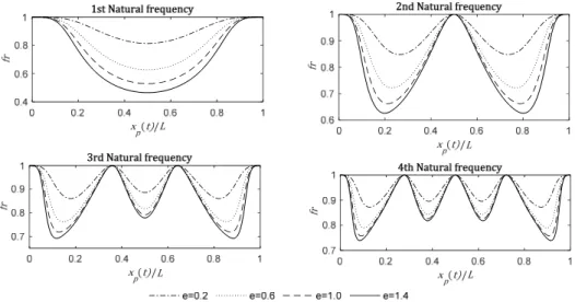
In moving mass problem, the variation of the natural frequencies of the beam is an interesting phenomenon that every design engineer should take into account of this effect of the mass. When the mass moves on the beam depending on the position of the mass, the natural frequencies undergo a continuous change, thus the vibration of the beam has to change as can be seen in Figures 3-7 in which normalized frequencies fr versus normalized position xp (t)/L of the mass over the beam are
depicted for different end support conditions. Where fr is ratio of the frequencies in cases of with and
without mass on the beam.
Figure 3 displays the variation of the first four natural frequencies depending on the mass position on the beam and the mass ratio of the moving mass and the mass of the beam. Because of this variation in frequencies, the vibration behaviour of the beams under moving loads are very compli-cated and depends upon various parameters of the system such as mass, velocity, acceleration, and jerk of the moving mass including end support conditions. The variation of a particular natural fre-quency is governed by its corresponding natural mode shape. For example, as can be seen from Figure 3 the variation of the first natural frequency resembles its first natural mode shape. This is also valid for the other natural frequencies, 2nd, 3rd, 4th and so on. Another interesting behaviour is that at the location of the nodes, there are no changes of the frequencies even for higher mass ratios. Between the nodal points of the corresponding mode shapes, the rate of change is increased by the increasing mass ratio. These variations are also nonlinear, and have a tendency to the left or right as seen from the graphics depending on the first and last nodal point that are near to the left and right ends. The other nodal points except for these there are change but there is no tendency to the right or to the left. This event is valid for other end support conditions that are presented through Figures 3-7. The determination of the change in the natural frequencies is easy by using the proposed method in this study. Because the added matrices ofmw,mw,cw,cw, kw , kwand kG are always added to the left
side of the motion equation (19) of the whole system. This is the most advantageous property of the proposed method that one can directly model a dynamic system by including the inertia, Coriolis and centripetal forces and jerks of the moving mass as internal forces, and imposing the gravitational force to the right as an external force. The above matrices represent the dynamic added mass, damping and stiffness properties of the beam under a moving mass. The main difference of the assumption of the moving mass is this modification of the unloaded beam matrices. In the moving load assumption, all these matrices are zero except for the stiffness matrix kGdue to axial force effect in the flexural
deflection of the beam if there is an accelerating mass. Including second and third derivations of the deflection function one can analyse the effects of mass moving with constant and variable velocity on a beam using the current method.
Figure 4: Variations in natural frequencies for fixed-pinned beam.
/
0 0.2 0.4 0.6 0.8 1
0.4 0.6 0.8 1
/
0 0.2 0.4 0.6 0.8 1
0.6 0.8 1
/
0 0.2 0.4 0.6 0.8 1
0.6 0.8 1
/
0 0.2 0.4 0.6 0.8 1
0.7 0.8 0.9 1
Figure 5: Variations in natural frequencies for fixed-fixed beam.
Figure 6: Variations in natural frequencies for fixed-free beam.
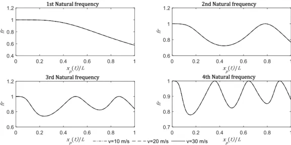
Figure 7: Variations in natural frequencies for fixed-free beam for e=0.5 and v=10, 20 and 30 m/s.
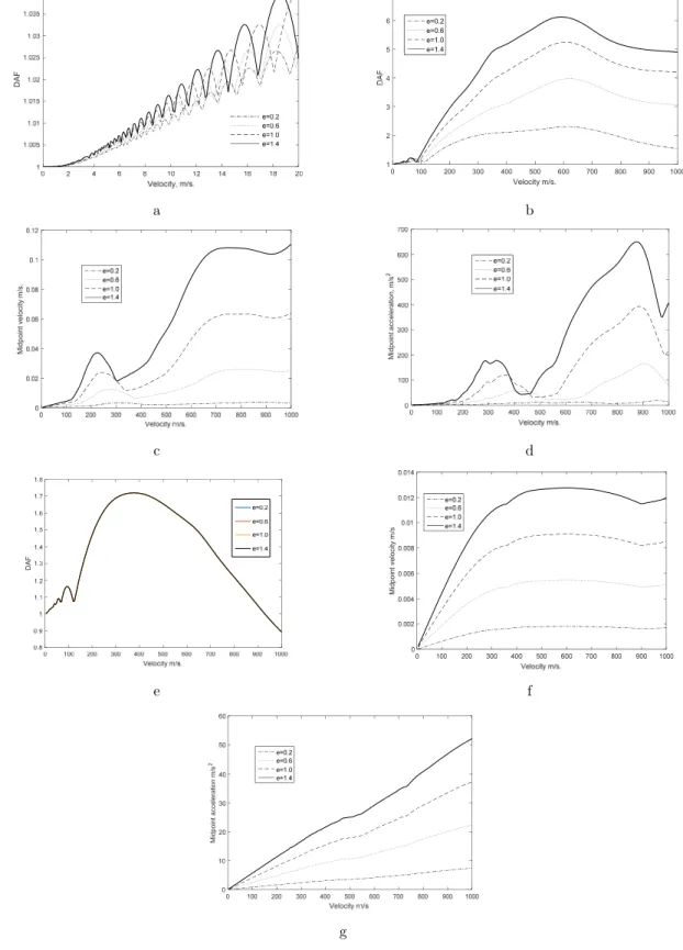
Moving load problems have been studied widely in literature, but most of these studies are for vehicle bridge interaction; and the most of them have omitted the inertial effect of the mass and accepted only the gravitational force of the moving load. Some of them have been modelled as moving oscillator that the main mass of the load is modelled as a sprung mass, and the unsprung mass of the suspension system is omitted. However, for the application of CNC applications of the moving mass where the accuracy of the work piece is important all the mass of the moving load is firmly in contact with the beam, the dynamic amplification factor (DAF) for different masses of the moving load may be significant for design engineers. Where DAF= maximum dynamic displacement of the beam/static displacement of the beam when the mass is at the middle. Figure (8) displays the DAF’s, and vibra-tion acceleravibra-tion and velocities of the midpoint for different constant travelling velocities of the mass and different mass ratios e, where e= mass of the moving load/mass of the beam. The mass of the given beam is 22.2 kg; and for e=0.2, 0.6, 1.0 and 1.4, the masses of the moving load are: 4.44, 13.32, 22.2 and 31.08 kg, such a mass ratio applies to CNC applications. Figure (8a) is for lower velocities while the others are for higher velocities. The figures (8e, 8f and 8g) are for moving load assumptions which the inertia, Coriolis and centripetal effects of the moving mass are omitted and only gravita-tional effect is considered, while Figures (8a to 8e) are for moving mass assumption that consider all the effects of the moving mass. From the figures, one can realize that they are very different in terms of the mentioned assumptions. The maximum DAF is about 1.7 for moving load assumption, but for the moving mass assumption it is about 6 that is higher about 3.53 times. This is due to the effect of mass with higher travelling velocities. For very low travelling velocities the difference is not consid-erably high when the rigidity of the beam is high in comparison with the velocity due to its little effect in the system mass, stiffness and damping matrices. The velocity increment in Figure (8a) is 0.001 m/s, while it is 5 m/s for the others. When Figure 8a, is examined closely, it is observed that there are many resonance peaks and cancellation points.
/
0 0.2 0.4 0.6 0.8 1
0.4 0.6 0.8 1 1.2
/
0 0.2 0.4 0.6 0.8 1
0.6 0.8 1 1.2
/
0 0.2 0.4 0.6 0.8 1
0.6 0.8 1 1.2
/
0 0.2 0.4 0.6 0.8 1
0.7 0.8 0.9 1
a b
c d
e f
g
Figure 8: Comparisons of DAFs in moving mass (a, b, c and d) and moving load (e, f and g) assumptions.
D
AF
Velocity m/s.
0 100 200 300 400 500 600 700 800 900 1000 1
2 3 4 5 6 7
e=0.2 e=0.6 e=1.0 e=1.4
M
id
po
in
t v
el
oci
ty
m/
s.
Mi
dp
oi
nt
a
cce
le
ra
tio
n,
m
/s
2
D
AF
M
id
po
in
t v
el
oci
ty
m
/s
Mi
dp
oi
nt
a
cc
el
er
at
io
n
m/
s
In both cases the vibration acceleration and velocities are very different from each other. In the case of the moving mass in Fig. 8d, the maximum is ten times higher when compared to the moving load case in Fig. 8g. In addition, although the increase in the mass ratio is linear, the increase in the maximum of the moving mass is not linear, but the increase in the moving load is linear in acceleration and speed, but no increase is observed in the DAF that there is no difference with increasing mass ratio e. The effect of the mass on the frequency variation of the beam given in Figure 3-8 is valid for the moving mass assumption. At constant acceleration of the mass, the displacements and rotations at the midpoint of the beam are given in Fig. 9. The increase in displacement seems to be very high at high acceleration of motion. However, such high acceleration cannot be the case for CNC applica-tions. In addition, from the standpoint of existing bridge engineering problems, high acceleration does not apply in existing applications. However, the acceleration effect can be accounted for in high speed rail transport applications. Moreover, if the projectile is considered that accelerations to be higher than the given examples, the impact of the exposure should be considered in such applications, in the case of projectile and barrel interaction.
a b
c d
Figure 9: Midpoint displacements and rotations for e=1, and different constant acceleration.
xp(t)/L
0 0.2 0.4 0.6 0.8 1
M
id
po
in
t d
isp
la
ce
m
en
t (
m
)
10-6
-1 0 1 2 3 4 5 6
a= a= a= a=
xp(t)/L
0 0.1 0.2 0.3 0.4 0.5 0.6 0.7 0.8 0.9 1 10-5
-8 -6 -4 -2 0 2 4 6 8
a=5e4 a=1.5e5 a=2.5e5 a=3.5e5
xp(t)/L
0 0.2 0.4 0.6 0.8 1
10-6
-2.5 -2 -1.5 -1 -0.5 0 0.5 1 1.5 2 2.5
a=5 a=15 a=25 a=35
xp(t)/L
0 0.1 0.2 0.3 0.4 0.5 0.6 0.7 0.8 0.9 1 10-4
-2 0 2 4 6 8 10 12
The jerk can be valid for a sudden acceleration increase takes place in braking or accelerating due to the applied force chances over time. Starting with zero acceleration at different jerks, displacements of the midpoint of the beam are illustrated in Figure 10. For the movement with little jerks, Figure 10 a, the displacements are not significantly changed but for higher jerks, Figure 10b, as it can be in projectile motion in a barrel it is observed that displacements are considerably increased.
a b
Figure 10: Midpoint displacements for e=1, and different constant Jerks.
When the mass moves with an acceleration due to an axial force is applied at the contact point of the mass, the beam vibrates in axial direction. Figure 11 shows the axial displacements of the midpoint for e=1, and case of different lower accelerations in (a), and case of different higher accel-erations in (b). Higher accelaccel-erations are valid for projectile and barrel interaction of a weapon system like a tank that the exit velocity of the projectile is about 1750 m/s. One can calculate the average acceleration of the projectile that starts from zero velocity to a 1750 m/s exit velocity in a 6 m long barrel, the average acceleration is 2.55e5 m/s2. For lower accelerations that can be applicable for CNC applications the midpoint displacements are increased by the increasing of the motion acceleration of the mass. The rate of displacement increase should be considered when the accuracy of the work is important.
Figure 11: Axial displacements of midpoint for e=1, and different constant accelerations.
xp(t)/L
0 0.2 0.4 0.6 0.8 1
M
id
po
in
t d
is
pl
ace
m
en
t (
m
)
10-6
-1 0 1 2 3 4 5 6
J=1 J=10 J=20 J=30
Mi
dp
oi
nt
d
isp
la
ce
me
nt
m.
xp(t)/L
0 0.2 0.4 0.6 0.8 1
10-7
-2 0 2 4 6 8 10 12 14
a=5 a=15 a=25 a=35
xp(t)/L
0 0.1 0.2 0.3 0.4 0.5 0.6 0.7 0.8 0.9 1 10-3
0 2 4 6 8 10 12 14 16 18 20
In terms of bridge engineering applications, the effect of axial forces may be significantly lower due to the motion acceleration of the vehicle, but this effect may be important for asphalt life. Another application of accelerated motion is rocket launching, where a massive mass can experience very high acceleration because of the ignition of a rocket.
4 CONCLUSIONS
In this study, the inertial, Coriolis and centripetal effects of the moving mass are determined in terms of variable acceleration and constant jerk. The classical beam element equations are modified from the terms that come from the moving mass. The variable acceleration and jerk of the mass are com-bined the accelerations and jerks of the beam element on which the mass locates at time t, at the variable contact point of the mass. This method, in which only the contact element is replaced and the other elements of the beam remain the same, is a very advantageous tool for calculating many motion patterns, including jerk effect. In the formulation of the time-dependent force equation of the contacted beam element, the effects of velocity, acceleration and jerk are separately determined in order to investigate separately the effects of them. Some interesting results of the different cases are presented in terms of the usage field of the moving load problem, including the possible application of the theory in design of runways of CNCs, vehicle-bridge-interaction, in design of the barrels and rocket launching structures under the effect higher acceleration and jerks, etc. The general approach in Bridge design, the DAF is criticized, in terms of omitting the mass inertia and accepting the moving mass as a moving load that accepts the only gravitational effect of the mass. It is shoved that, for lower velocity of travelling of the mass, this approach makes not very much difference, but for higher velocities and accelerations, including the inertial effect, the DAF can be three times greater depend-ing on size of the velocity, acceleration, and jerk. One drawback of the proposed method is that it is not usable for hand calculations due to the modification of the system matrices in each time step of the integration.
References
Awodola, T. O., 2014, 2014. Flexural motions under moving masses of elastically supported rectangular plates resting on variable winkler elastic foundation, Lat. Am. J. Solids. Stru. 11, 1515-1540.
Bathe, K. J., 1996. Finite element procedures in engineering analysis, 2nd Ed, Prentice Hall, New Jersey, 1996. Cifuentes, A. O. 1989. Dynamic response of a beam excited by a moving mass, Finite Elem. Anal. Des. 5, 237– 246. Clough R.W; Penzien J., 2003. Dynamics of Structures, Dynamics of Structures. doi:10.1002/9781118599792
Dehestani, M., Mofid, M., Vafai, A., 2009. Investigation of critical influential speed for moving mass problems on beams. Appl. Math. Model. 33, 3885–3895. doi:10.1016/j.apm.2009.01.003
Dyniewicz, B., Bajer, C. 2012. New consistent numerical modelling of a travelling accelerating concentrated mass, World J. Mech. 2 (6), 281-287.
Esen, I., 2011. Dynamic response of a beam due to an accelerating moving mass using moving finite element approximation. Math. Comput. Appl. 16, 171–182.
Esen, I., 2013. A new finite element for transverse vibration of rectangular thin plates under a moving mass. Finite Elem. Anal. Des. 66, 26–35. doi:10.1016/j.finel.2012.11.005
Esen, I., Koç, M.A., 2015b. Dynamic response of a 120 mm smoothbore tank barrel during horizontal and inclined firing positions. Lat. Am. J. Solids Struct. 12, 1462–1486.
Esen, I., 2015. A new FEM procedure for transverse and longitudinal vibration analysis of thin rectangular plates subjected to a variable velocity moving load along an arbitrary trajectory. Lat. Am. J. Solids Struct. 12, 808–830. Fryba, L. 1999.. Vibration solids and structures under moving loads. Thomas Telford House.
Gerdemeli, I., Esen, I., Ozer, D., 2011. Dynamic Response of an Overhead Crane Beam Due to a Moving Mass Using Moving Finite Element Approximation, Key Eng. Mat. 450, 99-102.
Kadivar, M.H., Mohebpour, S.R., 1998. Finite element dynamic analysis of unsymmetric composite laminated beams with shear effect and rotary inertia under the action of moving loads. Finite Elem. Anal. Des. 29, 259–273. doi:10.1016/S0168-874X(98)00024-9
Kahya, V., 2012. Dynamic analysis of laminated composite beams under moving loads using finite element method. Nucl. Eng. Des. 243, 41–48. doi:10.1016/j.nucengdes.2011.12.015
Lee, H. P., 1996. Transverse vibration of a Timoshenko beam acted upon by an accelerating mass, Appl. Acoust. 47 (4), 319-330.
Meirovitch, L., 1967. Analytical methods in vibrations. The Macmillan Company, New York.
Michaltsos, G., Sophianopoulos, D., Kounadis, A.N., 1996. The Effect of a Moving Mass and Other Parameters on the Dynamic Response of a Simply Supported Beam. J. Sound Vib. 191, 357–362. doi:10.1006/jsvi.1996.0127
Michaltsos, G. T, Kounadis, A. N., 2001. The effects of centripetal and Coriolis forces on the dynamic response of light bridges under moving loads, J. Vib. Control 7, 315-326.
Michaltsos, G,T., 2002. Dynamic behaviour of a single-span beam subjected to loads moving with variable speeds. J. Sound Vib. 258, 359–372. doi:10.1006/jsvi.5141
Mizrak, C., Esen, I., 2015. Determining Effects of Wagon Mass and Vehicle Velocity on Vertical Vibrations of a Rail Vehicle Moving with a Constant Acceleration on a Bridge Using Experimental and Numerical Methods, Shock. Vib. Doi: http://dx.doi.org/10. 1155/2015/183450.
Mohebpour, S. R., Malekzadeh, P., Ahmadzadeh, A. A., 2011. Dynamic analysis of laminated composite plates sub-jected to a moving oscillator by FEM, Compos. Struct. 93, 1574–1583.
Nikkhoo A., Rofooei, F. R., Shadnam, M. R., 2007. Dynamic behaviour and modal control of beams under moving mass, J. Sound Vib. 306, 712-724.
Omolofe, B., 2013. Deflection profile analysis of beams on two-parameter elastic subgrade, Lat. Am. J. Solids Stru. 10, 263 – 282.
Oni, S. T., Awodola, T. O., 2010. Dynamic response of an elastically supported non-prismatic beam on variable elastic foundation, Lat. Am. J. Solids Stru. 7, 3 – 20.
Sharbati, E., Szyszkowski, W., 2011. A new FEM approach for analysis of beams with relative motions of masses, Finite Elem. Anal. Des. 47, 1047-1057.
Szilard R., 2004. Theories and Applications of Plate Analysis, Wiley, New Jersey.
Wang, Y., 2009. The transient dynamics of a moving accelerating / decelerating mass traveling on a periodic-array non-homogeneous composite beam. Eur. J. Mech. A/Solids 28, 827–840. doi:10.1016/j.euromechsol.2009.03.005 Wilson, E.L., 2002. Static and Dynamic Analysis of Structures. Computers and Structures Inc., Berkeley. Wu J. J., 2005. Dynamic Analysis of an inclined beam due to moving loads, J. Sound Vib. 288, 107-131.
APPENDIX A
Derivation of Eqs. (6) and (9):
When the beam is in vibration, the longitudinal (x) force component, between the moving mass and the beam, induced by the vibration and curvature of the deflected beam is
(
)
2
2
d ( , )
( , ) ( ) ( ),
d
x p
t t t t
x p p p p x p
w x t
f x t m a x x m a J t m w x x
t d d
-D
æ ö÷
ç ÷
ç
= çç - ÷÷ - = - + D +
-÷÷
çè ø (A.1)
The axial acceleration of the beam is derived from the second order total differentiation of its deflection function wx =w x tx( , ) with respect to time dependent contact point xp as given below:
2
d ( , ) ( , )d ( , )
( , ) ( , ) ( , ),
d d
d ( , ) ( , )d ( , )
( , ) ( , ) ( , ),
d d
p
p
x x x
x x x
x x
x x x
x x x
x x w x t w x t x w x t
vw x t w x t w x t
t x t t
w x t w x t x w x t
vw x t w x t w x t
t x t t
= = ¶ ¶ ¢ = + = + » ¶ ¶ ¶ ¶ ¢ = + = + » ¶ ¶ (A.2)
When the beam is in vibration, thetransverse (z) force component, between the moving mass and the beam, induced by the vibration and curvature of the deflected beam is
(
)
2 3
2 3
d ( , ) d ( , )
( , ) ,
d d
t
t t
z p z p
t
z p p
w x t w x t
f x t m g t x x
t t d
-D
é æ öù
ê çç ÷÷ú
ê ç ÷ú
= ê -ç + D ÷÷ú
-ç ÷
ê ççè ÷øú
ê ú
ë û
(A.3)
The vertical acceleration of the beam is derived from the second order total differentiation of its deflection function wz =w x tz( , ) with respect to time dependent contact point xp and the jerk from
its time derivative as given below:
2
2 2 2 2 2
2 2 2 2
2
3
3 3
3 3
d ( , ) ( , )d ( , )
,
d d
d ( , ) ( , ) ( , )d ( , ) d ( , )d
2 ,
d d
d d
2 ,
d ( , ) d
d d
p
p
z z z
x x
z z z z z
x x
z z z z
z z
w x t w x t x w x t
t x t t
w x t w x t w x t x w x t x w x t x
x t t t x
t t x t
w vw v w aw
w x t w x
t t x = = ¶ ¶ = + ¶ ¶ æ ö
¶ ¶ ¶ ç ÷÷ 
= + + ççç ÷÷ +
¶ ¶ 
¶ ¶ è ø
¢ ¢¢ ¢
= + + +
æ ö
¶ ç ÷÷
= ççç ÷÷
¶ è ø
2
3 2 2 3
2 2 2
2 2 3 3
2 3 3
3 2
d d d d
3 3 3
d d d d ,
d d
d d
3 3 3
p
z z z
z z z
x x
z z z z
w x w x x w x
t t t t
x t x t x
w x w x w
x t t x t x
w v w v w va w v
=
æ ö
¶ ç ÷÷ ¶ 
+ ççç ÷÷ + +
¶ ¶ è ø ¶ ¶ 
¶ ¶ ¶ + + + ¶ ¶ ¶ ¶ ¢¢¢ ¢¢ ¢¢ ¢ = + + + + 2 3 2 3 ,
d d d
; ;
d d d
p p p
z z z
x x x x x x
w a Jw w
x x x
v a J
t = t = t =
¢ + ¢+
= = =