M
ASTER OF
S
CIENCE IN
M
ONETARY AND
F
INANCIAL
E
CONOMICS
M
ASTERS
F
INAL
W
ORK
D
ISSERTATION
A
SSESSING
P
UBLIC
S
PENDING
E
FFICIENCY IN
20
OECD
C
OUNTRIES
M
INA
K
AZEMI
S
UPERVISOR:
A
NTÓNIOA
FONSOM
ESTRADO
M
ONETARY AND
F
INANCIAL
E
CONOMICS
T
RABALHO
F
INAL DE
M
ESTRADO
D
ISSERTAÇÃO
A
SSESSING
P
UBLIC
S
PENDING
E
FFICIENCY IN
20
OECD
C
OUNTRIES
M
INA
K
AZEMI
S
UPERVISOR:
A
NTÓNIOA
FONSOAbstract
Being allocated a large share of a country’s GDP to the public spending, would rise the question of whether these resources are distributed and allocated in an efficient manner that leads the country to go through the growth enhancing economic path or not. This study is mainly going to follow Afonso, Schuknecht, and Tanzi (2005), aiming to look at the public expenditure of 20 OECD countries for the period 2009-2013, from the perspective of efficiency and assess if these developed countries are performing efficiently compared to each other. In order to evaluate the efficiency scores, Public Sector Performance (PSP) and Public Sector Efficiency (PSE) indicators were constructed and Data Envelopment Analysis was conducted. The results of these analyses show that the only country that performed on the efficiency frontier is Switzerland. The average input-oriented efficiency score is equal to 0.732. That is, on average countries could have reduced the level of pub-lic expenditure by 26.8% and still achieved the same level of pubpub-lic performance. The av-erage output-oriented efficiency score is 0.769 denoting that on avav-erage the sample coun-tries could have increased their performance by 23.1% by employing the same level of public expenditure.
Keywords: Public Spending, Technical Efficiency, Public Sector Performance (PSP), Data Envelopment Analysis (DEA)
Contents
1. Introduction 1
2. Literature review 3
3. Methodology 7
3.1. Public Sector Performance (PSP) 7
3.2. Public Sector Efficiency (PSE) 9
3.3. Data Envelopment Analysis (DEA) 10
4. Empirical analysis 12
4.1. Public Sector Performance (PSP) 13
4.2. Public Sector Efficiency (PSE) 16
4.3. Data Envelopment Analysis (DEA) 19
5. Conclusions 27
References 29
1
1. Introduction
Being the main element in the policy-making decisions, governments have a great
respon-sibility to move the countries towards economic growth and to increase the social welfare.
Confronting the constant budget constraints and employing the correct policies by
gov-ernments is one of the crucial issues due to the pressures from globalization and ageing
population on the countries budget on both expenditure and revenue sides (Deroose and
Kastrop (2008)). As a large share of the GDP is allocated to the public spending, improving
the public spending efficiency is an important issue that could help to ensure the
sustain-ability of the public finances (Barrios and Schaechter (2008)). Understanding how far the
governments can increase their performance at the same spending levels simply by
in-creasing their spending efficiency could help fiscal policy makers achieving sustained fiscal
disciplines (Mandl, Dierx, and Ilzkovitz (2008)) .
This study is going to assess the public spending efficiency in 20 OECD countries during the
period 2009-2013. The main reason of doing this work is to recognize how well and
effi-cient these countries are performing from both input and output perspectives. First we
constructed the composite indicators on Public Sector Performance (PSP) and computed
the Public Sector Efficiency (PSE), and then we implemented a non-parametric approach
called Data Envelopment Analysis (DEA) for 6 different models. The first two models are
considering the efficiency of the government in a macro level and the other four models
assess the efficiency of public expenditure in four different core areas of government
2
This work follows Afonso, Schuknecht, and Tanzi (2005) with a slightly smaller
country-sample due to the data availability, but with more recent data, and substituting FDH with
the DEA approach. The reason that we preferred DEA to FDH is the higher accuracy of the
DEA in the results due to the convexity assumption.
DEA results obtained from running model 1 and 2 show that Switzerland by applying the
lowest amount of public expenditure could achieve the highest level of performance in
this sample and it’s the only country that is performing on the efficiency frontier with a
significant distance from the other countries. The results of running the DEA for the other
models suggest that governments of these countries are performing more efficiently in
the health and education systems than in the administration and infrastructure functions.
Our results are highly in line with the results of the previous studies in this subject (e.g. St.
Aubyn et al. (2009), Afonso, Schuknecht, and Tanzi (2005), etc.) suggesting that the
gov-ernments could get a higher level of performance by spending at the same level or that
they could obtain the same level of performance by spending less. The average
input-oriented efficiency score is equal to 0.732. That is, on average countries could have
re-duced the level of inputs by 26.8% and achieve the same outputs. The average
output-oriented efficiency score is 0.769 denoting that on average the countries could have
in-creased the level of their outputs by 23.1% by employing the same level of inputs.
The next chapter is a literature review. Chapter three introduces the methodology that is
used. Chapter four describes the results of the assessment and finally chapter five
3
2. Literature Review
The literature on assessing the government spending efficiency has usually obtained the
efficiency frontiers either by applying parametric or non-parametric approaches.
Stochas-tic Frontier Analysis (SFA) is a popular parametric approach and Free Disposal Hull (FDH)
and Data Envelopment Analysis (DEA) are the two non-parametric approaches that have
been used by many researchers in order to obtain an efficiency frontier. It is worth
men-tioning that there haven’t been too many studies in evaluating the public spending
effi-ciency at an aggregate level.
Herrera and Pang (2005), applied FDH and DEA methodologies to compute the input and
output efficiency scores of health and education public sectors of 140 countries for the
period 1996 to 2002. Their results indicate that countries with higher spending levels
ob-tained lower efficiency scores.
Afonso and St. Aubyn (2005), assessed the efficiency of the public spending for the
educa-tion and health sectors across 17 and 24 OECD countries in 2000. They applied FDH and
DEA approaches in order to compare the results of each method. For the education
analy-sis they used hours per year in school and teachers per 100 students as inputs and PISA
scores as output. For the health analysis they used the number of doctors, nurses and
beds as inputs and infant survival and life expectancy as outputs. The results related to the
comparison of these two techniques infer that some of the countries that were
consid-ered as efficient under FDH are no longer efficient according to the DEA results, and that
4
Afonso, Schuknecht, and Tanzi (2005), computed the Efficiency scores for 23 OECD
coun-tries for 1990 and 2000 by constructing the PSP indicators and considering the PSP scores
as an input measure and public expenditure as percentage of GDP as an output measure
by applying the FDH methodology. The results of their studies show that small
govern-ments obtained better performance and efficiency scores compared to the larger ones.
And larger governments could have obtained the same level of performance by decreasing
the level of the public expenditure.
Sutherland et al. (2007), applied both non-parametric (DEA) and parametric (SFA)
ap-proaches to assess the public spending efficiency in primary and secondary education
among OECD countries. The results of school-level efficiency estimated by them suggest a
high correlation between the results of both approaches. Their results show that
govern-ments could gain higher efficiency scores by decreasing the expenditure levels and
keep-ing the performance constant.
Afonso and Fernandes (2008), assessed the public spending efficiency of 278 Portuguese
municipalities for the year 2001 by applying a non-parametric approach (DEA). They
con-structed a composite indicator of local government performance and considered it as the
output measure and the level of per capita municipal spending as the input measure of
the DEA. The results of the DEA implemented by them suggest that most of these
munici-palities could have achieved the same level of performance by decreasing the level of the
5
St. Aubyn et al. (2009), applied a two stage semi-parametric (DEA and the Tobit
regres-sion) and a parametric approach (SFA) in order to evaluate the efficiency and effectiveness
of public spending on tertiary education for 26 EU countries plus Japan and the US for two
different periods (1998-2001 and 2002-2005). They conclude that to be considered as
good performers countries do not necessarily need to increase their spending on higher
education but need to spend efficiently.
Afonso, Romero, and Monsalve (2013), computed the Public Sector Efficiency (PSE) and
conducted a DEA in order to assess the public expenditure efficiency for 23 Latin American
and Caribbean countries for the period 2001-2010. The output measure suggested by
them is the Public Sector Performance (PSP) scores computed by constructing the
compo-site indicator of public sector performance. The input measure is the total public
spend-ing-to-GDP ratio. They conclude that the PSE scores have an inverse correlation with the
size of the governments and also that these governments could achieve the same level of
output with less government spending.
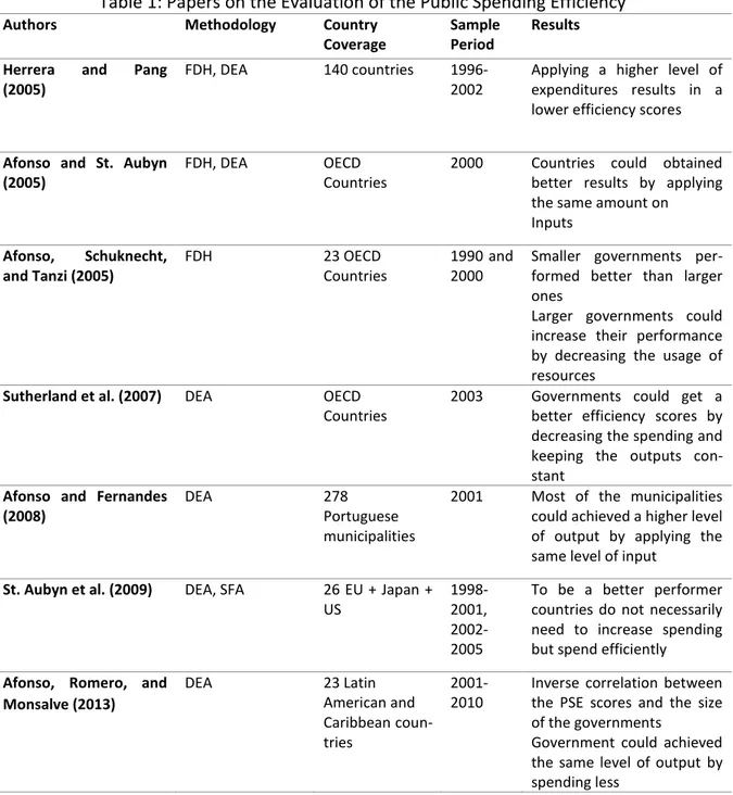
Table 1 summarizes all the literature we mentioned above with their results and specific
6
Table 1: Papers on the Evaluation of the Public Spending Efficiency
Authors Methodology Country
Coverage
Sample Period
Results
Herrera and Pang (2005)
FDH, DEA 140 countries 1996-2002
Applying a higher level of expenditures results in a lower efficiency scores
Afonso and St. Aubyn (2005)
FDH, DEA OECD
Countries
2000 Countries could obtained better results by applying the same amount on Inputs
Afonso, Schuknecht, and Tanzi (2005)
FDH 23 OECD
Countries
1990 and 2000
Smaller governments per-formed better than larger ones
Larger governments could increase their performance by decreasing the usage of resources
Sutherland et al. (2007) DEA OECD Countries
2003 Governments could get a better efficiency scores by decreasing the spending and keeping the outputs con-stant
Afonso and Fernandes (2008)
DEA 278
Portuguese municipalities
2001 Most of the municipalities could achieved a higher level of output by applying the same level of input
St. Aubyn et al. (2009) DEA, SFA 26 EU + Japan + US
1998-2001, 2002-2005
To be a better performer countries do not necessarily need to increase spending but spend efficiently
Afonso, Romero, and Monsalve (2013)
DEA 23 Latin
American and Caribbean coun-tries
2001-2010
Inverse correlation between the PSE scores and the size of the governments
7
3. Methodology and Data
This study’s Database is compiled from various sources that are listed in table A1 and table
A2 (in the Appendix). Table A1 lists several sub-indicators that are used for constructing
the PSP indicators. These PSP indicators are then used as the output measure for the
fron-tier analysis. Table A2 includes the data on various governments’ expenditures area, which
then could be used as the input measures for the efficiency analysis.
The methodology applied in this study includes three approaches. The first two sections
explain how the PSP and PSE are constructed and the third section provides an intuitive
approach to the Data Envelopment Analysis (DEA).
3.1. Public Sector Performance (PSP)
In order to compute the Public Sector Performance, we followed Afonso, Schuknecht, and
Tanzi (2005). They introduced the two main components of PSP, called opportunity
indica-tors and the traditional Musgravian indicaindica-tors.
The opportunity indicator that focuses on the role of the government in providing various
and accessible opportunities for individuals in the market place contains four
sub-indicators. These sub-indicators reflect the governments’ performance in four areas,
ad-ministration, education, health and infrastructure. The administration sub-indicator
com-prises the same indices as it had in Afonso, Schuknecht, and Tanzi (2005), which consists
of: corruption, burden of government regulation (red tape), judiciary independence and
shadow economy. Besides that, we added another component called the property rights
8
in increasing the welfare and economic growth by providing a reliable environment for
individuals and companies to invest. In order to measure the education sub-indicator, we
used the secondary school enrolment rate, quality of educational System and PISA scores.
For the health sub-indicator, we compiled data on the infant mortality rate and life
expec-tancy. The infrastructure sub-indicator is measured by the quality of overall infrastructure.
In order to focus on the structural changes we computed the 5-year (2009-2013) average
of all the indices in constructing the opportunity indicators.
The Musgravian Indicators consist of three sub-indicators: distribution, stability and
eco-nomic performance. In order to measure the PSP of distribution sub-indicator, we used
the 5-year average of the Gini Coefficient (2009-2013). For the stability sub-indicator, we
used the coefficient of variation of 10-year (2004-2013) GDP growth and standard
devia-tion of 10 years (2004-2013) infladevia-tion.
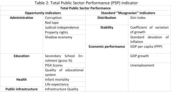
Table 2: Total Public Sector Performance (PSP) indicator
Total Public Sector Performance
Opportunity indicators Standard ‘’Musgravian’’ Indicators
Administrative Corruption Distribution Gini index
Red tape
Judicial independence Stability Coefficient of variation of growth
Property rights
Shadow economy Standard deviation of
Inflation
Economic performance GDP per capita (PPP)
Education Secondary School En-rolment (gross %)
GDP growth
PISA Scores Unemployment
Quality of educational system
9
Table 2 presents a list of the variables that we collected data on, in order to construct the
PSP indicators. After having collected all data on all of the sub-indicators, we normalized
all the measures by dividing the value of a specific country by the average of that measure
for all the countries in the sample, in order to provide a convenient platform for
compar-ing the results. The PSPs in each sub-indicator was then constructed by the aggregation of
the measures related to each sub-indicator, after assigning equal weights to them.
In order to compute the total Public Sector Performance, we gave equal weights to each
sub-indicator of opportunity and Musgravian indicators and aggregated them.
Assume there are 𝑝 countries with 𝑛 areas of performance, then we can determine the
overall performance of the country 𝑖 by:
𝑃𝑆𝑃𝑖 = ∑𝑛𝑗=1𝑃𝑆𝑃𝑖𝑗 , 𝑖 = 1, … , 𝑝 ; with 𝑃𝑆𝑃𝑖𝑗 = 𝑓(𝐼𝑘) (1)
where 𝑓(𝐼𝑘) is a function of k observable socio-economic indicators 𝐼𝑘.
3.2. Public Sector Efficiency
In order to compute the Public Sector Efficiency, we take into account the costs that
gov-ernments have in order to achieve a certain performance level. So, we now consider the
Public Expenditure as the input and relate that expenditure to its’ relevant PSP indicator.
We consider the government consumption as the input in obtaining the administrative
performance, government expenditure in education as the input for the education
per-formance, health expenditure is related to the health indicator of performance and public
investment is considered as the input for the infrastructure performance. For the
10
the income distribution. The stability and economic performance are related to the total
expenditure. Then we weigh each area of government expenditure to its’ relative output
and compute the Public Sector Efficiency for each indicator and also the total PSE of each
country as follows:
𝑃𝑆𝐸𝑖 = ∑ 𝑃𝑆𝑃𝐸𝑋𝑃𝑖𝑗 𝑖𝑗 𝑛
𝑗=1 , 𝑖 = 1, … , 𝑛. (2)
where 𝐸𝑋𝑃𝑖𝑗 denotes the government expenditure of the country 𝑖 in the area 𝑗.Table A3
presents data on different categories of public expenditure (% of GDP) for the sample
countries that are the computed 10-year average for the period 2004-2013.
3.3. Data Envelopment Analysis (DEA)
Data Envelopment Analysis (DEA) is an approach that assesses the relative performance
and efficiency of a set of Decision-Making Units (DMUs) by using the linear programming
methods in order to construct a production frontier. This method assumes the convexity
of the production frontier. DEA’s inceptions were first introduced by Farrell (1957) and the
term DEA was used and became popular for the first time by Charnes, Cooper, and Rhodes
(1978).
DEA can be conducted for the input and output-oriented analysis by assuming that the
technology is constant or variable return to scale (CRS or VRS). The constant return to
scale DEA model doesn’t consider the constraint of convexity and also under this
assump-tion, the efficiency scores achieved from the both input- and output-oriented
11
Suppose there are 𝐼 Decision-Making Units (DMU), each DMU uses 𝑁 inputs to produce 𝑀
outputs. If 𝑋 is the 𝑁 × 𝐼 input matrix and 𝑌 is the 𝑀 × 𝐼 output matrix for all the 𝐼 DMUs,
then 𝑥𝑖 is an input column vector and 𝑦𝑖 is an output column vector for the 𝑖-th DMU. So
for a given DMU the DEA model according to Charnes, Cooper, and Rhodes (1978) is as
follow:
𝑀𝑎𝑥∅,𝜆∅
Subject to −∅𝑦𝑖 + 𝑌𝜆 ≥ 0
𝑥𝑖 − 𝑋𝜆 ≥ 0 (3)
𝑛1′𝜆 = 1 𝜆 ≥ 0
where ∅ is a scalar and 1⁄∅ is the output-oriented efficiency score and satisfies
0 < 1 ∅⁄ ≤ 1. According to Farrel (1957), if the efficiency score of a DMU is equal to 1,
then the firm is performing on the efficiency frontier and considered as a technically
effi-cient firm.
𝜆 (𝐼 × 1) is a vector of constants that measures the weights for identifying the location of
the inefficient firms. The constraint 𝑛1′𝜆 = 1 is the convexity restriction imposed on the
12
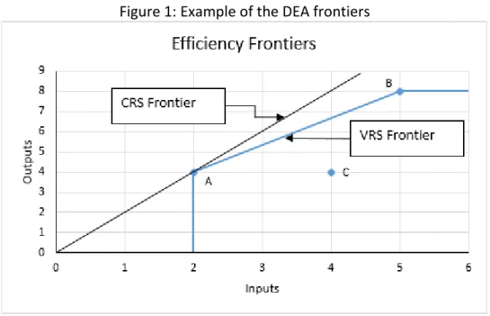
Figure 1: Example of the DEA frontiers
Figure 1 plots an example of the CRS and VRS DEA frontiers for three different firms. As
illustrated, firms A and B are located on the VRS efficiency frontiers so they are considered
as efficient DMUs. Firm A is considered efficient under CRS and VRS but firm B is not
per-forming efficiently under CRS. Firm C is considered inefficient because it could have
achieved a higher level of outputs by employing a lower level of inputs (Coelli et al.
(2005)).
4. Empirical analysis
The results are presented in 3 different sections. Section 4.1 presents the results from
constructing and evaluating the PSP indicator and scores. Section 4.2 provides the PSE
values and finally, section 4.3 represents the efficiency scores and results of the
13
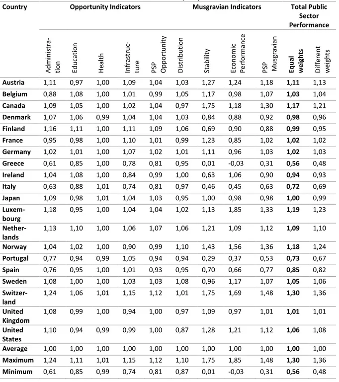
4.1. Public Sector Performance (PSP)
As we explained in the methodology section, we constructed the composite indicator on
the public sector performance by applying different variables for both Opportunity and
Musgravian indicators. Table 4 depicts the results of the PSP computations where
coun-tries with the PSP scores higher than 1 are considered as good performers. The PSP scores
range from 0.56 to 1.30 suggesting that Switzerland is the best performer and Greece is
the worst performer in the sample countries. The top 4 best performers are Switzerland,
Luxembourg, Norway and Canada. The worse performers according to the results are
Greece, Italy, Portugal and Spain.
Comparing the PSP results of each individual sub-indicator for different countries, we can
observe that Switzerland and Luxembourg are the best performers in the administration
area. Finland and the Netherlands are performing the best in education. In the provision
of health almost all of the countries are performing well. Switzerland and Finland are the
best performers in public infrastructure. We can also notice that in terms of income
distri-bution, Norway and Finland are performing the best, in terms of stability Switzerland and
14
Table 4: Public Sector Performance (PSP) Indicators, 2009-2013
Country Opportunity Indicators Musgravian Indicators Total Public Sector Performance Ad m in is tr a-ti o n E d u cat ion H e al th In fra stru c-tu re
PSP Op
p o rtu n ity Di stri b u ti o n Sta b il ity E con o m ic Perf o rm an ce
PSP Mu
sgrav ian E q u al we ig h ts Di ff e re n t w e ight s
Austria 1,11 0,97 1,00 1,09 1,04 1,03 1,27 1,24 1,18 1,11 1,13
Belgium 0,88 1,08 1,00 1,01 0,99 1,05 1,17 0,98 1,07 1,03 1,04
Canada 1,09 1,05 1,00 1,02 1,04 0,97 1,75 1,18 1,30 1,17 1,21
Denmark 1,07 1,06 0,99 1,04 1,04 1,03 0,84 0,88 0,92 0,98 0,96
Finland 1,16 1,11 1,00 1,11 1,09 1,06 0,69 0,90 0,88 0,99 0,95
France 0,95 0,98 1,00 1,10 1,01 0,99 1,23 0,85 1,02 1,02 1,02
Germany 1,02 1,01 1,00 1,07 1,02 1,01 1,11 0,96 1,03 1,02 1,03
Greece 0,61 0,85 1,00 0,78 0,81 0,95 0,01 -0,03 0,31 0,56 0,48
Ireland 1,04 1,08 1,00 0,84 0,99 1,00 0,63 1,06 0,90 0,94 0,93
Italy 0,63 0,88 1,01 0,74 0,81 0,97 0,46 0,45 0,63 0,72 0,69
Japan 1,09 0,98 1,01 1,04 1,03 0,95 1,00 0,98 0,98 1,00 0,99
Luxem-bourg
1,18 0,95 1,00 1,04 1,04 1,02 1,13 1,85 1,33 1,19 1,23
Nether-lands
1,13 1,10 1,00 1,06 1,07 1,06 1,21 1,09 1,12 1,09 1,10
Norway 1,04 1,02 1,00 0,90 0,99 1,10 1,43 1,56 1,36 1,18 1,24
Portugal 0,77 0,94 0,99 1,05 0,94 0,94 0,29 0,37 0,53 0,73 0,67
Spain 0,76 0,95 1,00 1,01 0,93 0,95 0,70 0,66 0,77 0,85 0,82
Sweden 1,08 1,00 1,00 1,03 1,03 1,08 0,96 1,17 1,07 1,05 1,06
Switzer-land
1,24 1,06 1,01 1,15 1,12 1,01 1,75 1,69 1,48 1,30 1,36
United Kingdom
1,08 0,99 1,00 0,94 1,00 0,97 1,09 0,97 1,01 1,01 1,01
United States
1,10 0,94 0,99 0,99 1,00 0,87 1,28 1,21 1,12 1,06 1,08
Average 1,00 1,00 1,00 1,00 1,00 1,00 1,00 1,00 1,00 1,00 1,00
Maximum 1,24 1,11 1,01 1,15 1,12 1,10 1,75 1,85 1,48 1,30 1,36
Minimum 0,61 0,85 0,99 0,74 0,81 0,87 0,01 -0,03 0,31 0,56 0,48
In order to check the robustness of the results and to check if different sub-indicators
have different impacts on the final results of the PSP scores, we assigned a higher weight
15
(instead of assigning equal weights to each indicator) by assuming that the Musgravian
indicators have higher impacts on the overall performance of the public sector of a
coun-try.
The results of the robustness analysis are very similar to the PSP scores computed by
as-signing equal weights to each indicator. The countries that obtained a PSP score higher
than average when assigning the equal weight to each indicator also achieved higher than
average performance results by assigning different weights to Opportunity and
Musgravi-an indicators. Similar results were also attained for the countries with a lower thMusgravi-an
aver-age PSP scores.
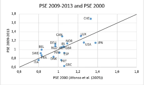
Figure 2: Comparison of our PSP results with the results obtained by Afonso, Schuknecht, and Tanzi (2005)
Figure 2 depicts the results of the Comparison of our PSP results with the results obtained
16
Switzerland, Canada, Norway, United States, Germany, Belgium, France and the United
Kingdom have improved their performance during these years.
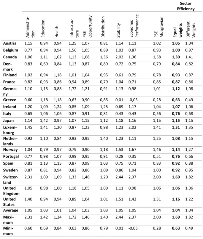
4.2. Public Sector Efficiency (PSE)
The following table shows the PSE scores that we computed by dividing the PSP scores of
each country for different sub-indicators by the level of the relevant expenditure category.
As we can see in Table 5, the PSE scores are ranging from 0.63 to 1.69. Switzerland is
con-sidered as the most efficient country among the 20 countries obtaining the PSE score of
1.69. On the other hand, Greece is considered as the least efficient country, obtaining a
PSE score equal to 0.63. The other efficient countries followed by Switzerland are
Luxem-bourg, Canada, Japan, Norway and Germany.
By considering the results of the computations of PSP and PSE at the same time, we can
find that countries such as France and Sweden that are considered as good performers are
not among the group of countries that are considered as efficient. Ireland on the other
hand is not considered as a very good performer but performs relatively efficiently. Figure
3 illustrates these results by defining four quadrants in which these countries are situated.
Comparing the PSE results with the results obtained from the earlier work of Afonso,
Schuknecht, and Tanzi (2005) on the OECD countries, we observe that Switzerland,
Lux-embourg, Canada, Norway, Ireland, Austria, Germany, Belgium, Sweden and France have
increased the level of their Public Sector Efficiency while the other countries obtained
17
Table 5: Public Sector Efficiency (PSE) Indicators, 2009-2013
Country Opportunity Indicators Musgravian Indicators Total Public Sector Efficiency Ad m in is tr a-ti o n E d u cat ion H e al th In fra stru c-tu re PSE Op p o rtu n ity Di stri b u ti o n Sta b il ity E con o m ic Perf o rm an ce PSE Mu sgrav ian E q u al we ig h ts Di ff e re n t Wei gh ts
Austria 1,15 0,94 0,94 1,25 1,07 0,81 1,14 1,11 1,02 1,05 1,04
Belgium 0,77 0,94 0,94 1,56 1,05 0,89 1,03 0,87 0,93 1,00 0,97
Canada 1,06 1,11 1,02 1,13 1,08 1,36 2,02 1,36 1,58 1,30 1,41
Den-mark
0,83 0,69 0,84 1,13 0,87 0,89 0,72 0,75 0,79 0,84 0,82
Finland 1,02 0,94 1,18 1,01 1,04 0,95 0,61 0,79 0,78 0,93 0,87
France 0,82 0,93 0,86 0,94 0,89 0,79 1,04 0,71 0,85 0,87 0,86
Germa-ny
1,10 1,15 0,88 1,72 1,21 0,91 1,13 0,98 1,01 1,12 1,08
Greece 0,60 1,18 1,18 0,63 0,90 0,85 0,01 -0,03 0,28 0,63 0,49
Ireland 1,20 1,09 1,24 0,85 1,09 1,25 0,69 1,17 1,04 1,07 1,06
Italy 0,65 1,06 1,06 0,87 0,91 0,81 0,43 0,43 0,56 0,76 0,68
Japan 1,14 1,42 0,97 1,07 1,15 1,12 1,18 1,16 1,15 1,15 1,15
Luxem-bourg
1,45 1,41 1,20 0,87 1,23 0,98 1,23 2,02 1,41 1,31 1,35
Nether-lands
0,92 1,10 0,84 0,93 0,95 1,40 1,23 1,11 1,25 1,08 1,15
Norway 1,04 0,79 0,97 0,79 0,90 1,18 1,53 1,67 1,46 1,14 1,27
Portugal 0,77 0,98 1,07 0,99 0,95 0,91 0,28 0,35 0,51 0,76 0,66
Spain 0,81 1,13 1,15 0,87 0,99 1,03 0,75 0,71 0,83 0,92 0,88
Sweden 0,87 0,81 0,94 0,82 0,86 1,09 0,86 1,04 1,00 0,92 0,95
Switzer-land
2,31 1,09 1,09 1,33 1,46 1,20 2,44 2,37 2,00 1,69 1,82
United Kingdom
1,05 0,98 1,00 1,18 1,05 1,09 1,11 0,98 1,06 1,06 1,06
United States
1,40 0,94 0,94 0,89 1,04 1,01 1,51 1,42 1,31 1,16 1,22
Average 1,05 1,03 1,01 1,04 1,03 1,03 1,05 1,05 1,04 1,04 1,04
Maxi-mum
2,31 1,42 1,24 1,72 1,46 1,40 2,44 2,37 2,00 1,69 1,82
Mini-mum
0,60 0,69 0,84 0,63 0,86 0,79 0,01 -0,03 0,28 0,63 0,49
18
Figure 3: Public Sector Performance and Public Sector Efficiency (2009-2013)
19
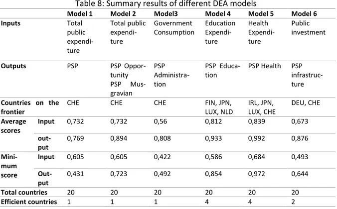
4.3. Data Envelopment Analysis (DEA)
We performed DEA for six different models assuming both constant and variable returns
to scale. The summary of the results of these models is reported in Table 8. Model 1
as-sumes 1 input (the governments’ normalized total spending) and 1 output (total PSP
scores). The results obtained from analysing model 1 are illustrated in Table 6. According
to these results, Switzerland is the only country that attains the efficiency score of 1, so it
is considered to be the most efficient country of the sample in terms of the public
ex-penditure. The least efficient country in the input-oriented analysis is France by attaining
the efficiency score of 0.605 meaning that France could have actually obtained the same
level of outputs by reducing the amounts of inputs by 39.5%. Considering the results of
the output-oriented analysis, Greece is attaining the efficiency score of 0.431, which leads
the country to be the least efficient among the other countries. This indicates that Greece
could have increased the outputs level by 56.9% and by consuming the same level of the
inputs.
The average input-oriented efficiency score is equal to 0.732. That is, on average countries
could have reduced the level of inputs by 26.8% and still achieve the same level of
out-puts. The average output-oriented efficiency score is 0.769 denoting that on average the
sample countries could have increased the level of their outputs by 23.1% by employing
20
Table 6: DEA results (Model 1), 2009-2013
Model 1 - 1 Input (Normalized Total Spending), 1 Output (Total PSP scores) COUNTRY CRS INPUT ORIENTED OUTPUT ORIENTED
VRS PEERS RANK VRS PEERS RANK Austria AUT 0,554 0,649 CHE 14 0,854 CHE 5 Belgium BEL 0,505 0,637 CHE 16 0,792 CHE 9 Canada CAN 0,745 0,828 CHE 4 0,9 CHE 4 Denmark DNK 0,464 0,615 CHE 19 0,754 CHE 15 Finland FIN 0,485 0,637 CHE 16 0,762 CHE 14 France FRA 0,475 0,605 CHE 20 0,785 CHE 10 Germany DEU 0,576 0,735 CHE 9 0,785 CHE 10 Greece GRC 0,272 0,632 CHE 18 0,431 CHE 20 Ireland IRL 0,572 0,791 CHE 5 0,723 CHE 16 Italy ITA 0,376 0,679 CHE 13 0,554 CHE 19 Japan JPN 0,652 0,847 CHE 2 0,769 CHE 13 Luxembourg LUX 0,724 0,791 CHE 5 0,915 CHE 2 Netherlands NLD 0,616 0,735 CHE 9 0,838 CHE 6 Norway NOR 0,695 0,766 CHE 8 0,908 CHE 3 Portugal PRT 0,389 0,692 CHE 12 0,562 CHE 18 Spain ESP 0,512 0,783 CHE 7 0,654 CHE 17 Sweden SWE 0,519 0,643 CHE 15 0,808 CHE 8 Switzerland CHE 1 1 CHE 1 1 CHE 1 United Kingdom GBR 0,565 0,727 CHE 11 0,777 CHE 12 United states USA 0,691 0,847 CHE 2 0,815 CHE 7 Average 0,569 0,732 0,769
Minimum 0,272 0,605 0,431
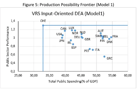
Figure 5 shows Model 1’s variable returns to scale efficiency frontier. As we can observe
Switzerland is the most efficient country and the only country that is performing on the
21
Figure 5: Production Possibility Frontier (Model 1)
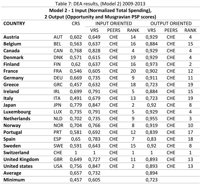
Model 2 assumes 2 outputs, the Opportunity PSP scores and the other one is the
Musgra-vian PSP scores and 1 input, the governments’ normalized total spending. According to the
results, Switzerland is the only efficient country and France (in the input-oriented analysis)
and Greece (in the output-oriented analysis) are again obtaining the least efficiency score
among all the countries. The results of this model are quite similar to the results we
ob-tained from implementing DEA on Model 1. The production possibility frontier of this
model is illustrated in Figure A1 in the Appendix. Due to the existence of two outputs and
one input we could only plot the production possibility frontier assuming that there exist
22
Table 7: DEA results, (Model 2) 2009-2013 Model 2 - 1 Input (Normalized Total Spending), 2 Output (Opportunity and Musgravian PSP scores)
COUNTRY CRS INPUT ORIENTED OUTPUT ORIENTED VRS PEERS RANK VRS PEERS RANK Austria AUT 0,602 0,649 CHE 14 0,929 CHE 4 Belgium BEL 0,563 0,637 CHE 16 0,884 CHE 15 Canada CAN 0,768 0,828 CHE 4 0,929 CHE 4 Denmark DNK 0,571 0,615 CHE 19 0,929 CHE 4 Finland FIN 0,62 0,637 CHE 16 0,973 CHE 2 France FRA 0,546 0,605 CHE 20 0,902 CHE 12 Germany DEU 0,669 0,735 CHE 9 0,911 CHE 11 Greece GRC 0,457 0,632 CHE 18 0,723 CHE 19 Ireland IRL 0,699 0,791 CHE 5 0,884 CHE 15 Italy ITA 0,491 0,679 CHE 13 0,723 CHE 19 Japan JPN 0,779 0,847 CHE 2 0,92 CHE 8 Luxembourg LUX 0,735 0,791 CHE 5 0,929 CHE 4 Netherlands NLD 0,702 0,735 CHE 9 0,955 CHE 3 Norway NOR 0,704 0,766 CHE 8 0,919 CHE 10 Portugal PRT 0,581 0,692 CHE 12 0,839 CHE 17 Spain ESP 0,65 0,783 CHE 7 0,83 CHE 18 Sweden SWE 0,591 0,643 CHE 15 0,92 CHE 8 Switzerland CHE 1 1 CHE 1 1 CHE 1 United Kingdom GBR 0,649 0,727 CHE 11 0,893 CHE 13 United states USA 0,756 0,847 CHE 2 0,893 CHE 13 Average 0,657 0,732 0,894
Minimum 0,457 0,605 0,723
DEA was also conducted for the other four models. These models try to evaluate the
effi-ciency of each country in different areas of governments’ performance. Table 8 shows the
summary of the results of these evaluations. Results of the Model 3 which focuses on the
administrative performance suggest that governments on average could have reduced the
level of their consumption by 44% and still got the same level of administrative
23
Model 4 results suggest that the same education performance could have been achieved
by lowering the level of expenditure on education. The results show that Finland, Japan,
Luxembourg and the Netherlands are performing on the efficiency frontier.
Model 5 considers the efficiency of the public health system. The results of the DEA
im-plemented on this model show that there exist four countries on the frontier that are
con-sidered to be efficient. These countries are Ireland, Japan, Luxembourg and Switzerland.
On average the sample countries could decreased the health expenditure by 16.1% and
attained the same level of health performance or they could had increased their
perfor-mance by 0.8% with the same level of health expenditure. This shows that these countries
on average are performing most efficiently in the health sector when compare to the
oth-er sectors.
The results of implementing DEA on Model 6 that considers the efficiency of public
infra-structure shows that Germany and Switzerland are the most efficient countries in the
sample in terms of public infrastructure, and on average all these governments could have
reached to the same level of infrastructure outputs by decreasing the public investment
by 32.7%.
These results also suggest that governments are performing more efficiently in the health
and education sections than in administrative and infrastructure sections despite the fact
that they apply a higher level of expenditure in administrative functions.
Due to the significant distance between the Switzerland’s efficiency score and the other
24
without considering Switzerland in the sample in order to acquire a more precise image of
the differences in the efficiency scores.
Table 8: Summary results of different DEA models
Model 1 Model 2 Model3 Model 4 Model 5 Model 6
Inputs Total
public expendi-ture Total public expendi-ture Government Consumption Education Expendi-ture Health Expendi-ture Public investment
Outputs PSP PSP
Oppor-tunity PSP Mus-gravian
PSP Administra-tion
PSP Educa-tion
PSP Health PSP infrastruc-ture
Countries on the frontier
CHE CHE CHE FIN, JPN,
LUX, NLD IRL, JPN, LUX, CHE DEU, CHE Average scores
Input 0,732 0,732 0,56 0,812 0,839 0,673
out-put
0,769 0,894 0,808 0,933 0,992 0,876
Mini-mum score
Input 0,605 0,605 0,422 0,586 0,684 0,493
Out-put
0,431 0,723 0,492 0,854 0,972 0,644
Total countries 20 20 20 20 20 20
Efficient countries 1 1 1 4 4 2
Table 9 shows the results of the recalculations of DEA for Model 1, excluding Switzerland
from the sample. These results denote the increase in the average efficiency scores of the
countries for both input and output oriented analysis. Model 1 as depicted in Figure 7,
suggests that Canada, Japan, Luxembourg and the United States are performing on the
efficiency frontier. Again, France and Greece are obtaining respectively the least input and
output oriented efficiency scores in both models. The countries on average could have
25
Table 9: DEA results (Model 1) excluding Switzerland, 2009-2013
Model 1- 1 Input (Normalized Total Spending), 1 Output (Total PSP scores)
COUNTRY Code CRT INPUT ORIENTED OUTPUT ORIENTED
VRT PEERS RANK VRT PEERS RANK
Austria AUT 0,736 0,769 CAN,USA 13 0,936 LUX 6
Belgium BEL 0,671 0,751 USA,JPN 15 0,866 LUX 9
Canada CAN 1 1 CAN 1 1 CAN 1
Denmark DNK 0,612 0,722 JPN 18 0,819 LUX 14
Finland FIN 0,643 0,751 JPN 15 0,828 LUX 13
France FRA 0,631 0,715 USA,JPN 19 0,854 LUX 11
Germany DEU 0,767 0,864 JPN,USA 9 0,859 LUX 10
Greece GRC 0,353 0,744 JPN 17 0,46 LUX 19
Ireland IRL 0,764 0,933 JPN 6 0,793 LUX,CAN 15
Italy ITA 0,494 0,8 JPN 12 0,597 LUX 18
Japan JPN 0,869 1 JPN 1 1 JPN 1
Luxembourg LUX 0,958 1 LUX 1 1 LUX 1
Netherlands NLD 0,82 0,87 CAN,USA 8 0,918 LUX 7
Norway NOR 0,93 0,949 LUX,CAN 5 0,994 LUX 5
Portugal PRT 0,515 0,816 JPN 11 0,61 LUX 17
Spain ESP 0,674 0,917 JPN 7 0,711 LUX 16
Sweden SWE 0,691 0,759 USA,JPN 14 0,882 LUX 8
United Kingdom GBR 0,75 0,859 USA,JPN 10 0,845 LUX 12
United states USA 0,925 1 USA 1 1 USA 1
MEAN 0,726 0,854 0,841
MINIMUM 0,353 0,715 0,46
26
Although Afonso, Schuknecht, and Tanzi (2005) applied a FDH approach in order to assess
the public spending efficiency and considered a bigger country-sample than what we did,
we take the opportunity to compare our results from DEA, with more recent data, with
the results they achieved from implementing FDH. By looking at Figure 8, we observe an
improvement in the efficiency scores of Canada, Finland, Germany, Italy, Netherlands,
Norway, Sweden and Switzerland during that 10-year period.
27
5. Conclusions
We assessed the public spending efficiency for 20 OECD countries for the period
2009-2013 by applying a non-parametric approach called Data Envelopment Analysis (DEA). In
order to do so first, we constructed the composite indicators of Public Sector Performance
(PSP) and Public Sector Efficiency (PSE) and then implemented the DEA approach for 6
different models by considering the level of the public spending as the input and the PSP
scores as the output of our analysis.
The derived PSP scores suggest that Switzerland is the best performer among all the other
countries in the sample followed by Luxembourg, Norway and Canada. The bottom
per-formers on the other hands are Greece, Italy, Portugal and Spain. France, Denmark,
Bel-gium, Finland, Sweden and Austria also could have performed the same by decreasing the
level of their total expenditure. Comparing these results with the results from Afonso,
Schuknecht, and Tanzi (2005) we can say that Switzerland, Canada, United Kingdom,
France, Belgium, Germany, Norway and United States had improved their performance
during this period of 10 years.
PSE results indicate that Switzerland is the most efficient country followed by Luxembourg
Canada, Japan, Norway and Germany. On the other hand Greece is considered as the least
efficient country. These results also propose that being a good performer doesn’t nece
s-sarily mean that the country is spending in an efficient manner. We can mention at France
and Sweden those of which are relatively good performers but not efficient countries.
28
public performance efficiency when comparing the results with the PSE results obtained
by Afonso, Schuknecht, and Tanzi (2005).
The results of the implemented DEA for model 1 that assesses the efficiency of the public
spending as a whole, show that the only country in this sample that is performing on the
efficiency frontier is Switzerland and all the other countries on average could decreased
the expenditure level by 26.8% and still attained the same level of performance.
According to what we observed by considering Switzerland as an outlier and excluding it
from the sample and recalculating the DEA scores, countries could got the same level of
outputs by decreasing the level of the public spending by 14.6%.
In summary, our results suggest that countries with a higher level of expenditures perform
less efficiently than countries that have a lower level of public spending. However,
follow-ing Mandl, Dierx, and Ilzkovitz (2008) we recommend individual analyses for each country
to complement our analysis due to the different traditions and cultures in institutional
settings, aspects of political economy, etc. and also applying a parametric analysis for
checking the robustness of the results could be strongly helpful for achieving sound fiscal
policies.
29
References
Afonso, A., Romero, A., and Monsalve, E. (2013). “Public Sector Efficiency : Evidence for
Latin America Public”. Inter-American Development Bank, 80478, Inter-American
De-velopment Bank. Department of Economics, ISEG-UL, Working Paper nº
19/2013/DE/UECE.
Afonso, A., and St. Aubyn, M. (2005). “Non-Parametric Approaches to Education and
Health Efficiency in OECD Countries.” Journal of Applied Economics VIII(2): 227–46.
Afonso, A., and Fernandes, S. (2008). “Assessing and Explaining the Relative Efficiency of
Local Government.” Journal of Socio-Economics 37(5): 1946–79.
Afonso, A., Schuknecht, L., and Tanzi, V. (2005). “Public Sector Efficiency: An International
Comparison.” Public Choice 123(3-4): 321–47.
St. Aubyn, M., Pina, A., Arcia, F. and Pais, J. (2009). “Study on the Efficiency and
Effectiveness of Public Spending on Tertiary Education”. Economic Papers no.390
Barrios, S., and Schaechter, A., (2008). “The Quality of Public Finances and Economic
Growth”. 337 European Commission, Economic and Financial Affairs Economic
Papers.
Charnes, A., Cooper, W. W. and Rhodes, E. (1978). “Measuring the Efficiency of Decision
Making Units”. European Journal of Operational Research 2(6): 429–44.
Coelli, T. J., Rao, D. S. P., O’Donnell, C. J., and Battese, G. E. (2005). “An Introduction to
30
Deroose, S., and Kastrop, C. (2008). “The Quality of Public Finances: Findings of the
Economic Policy Committee-Working Group (2004-2007)”. European Commission,
Economic and Financial Affairs Economic Papers.
Farrell, M. J. (1957). “The Measurement of Productive Efficiency”. Journal of the Royal
Statistical Society. Series A (General) 120(3): pp. 253–90.
Herrera, S., and Pang G. (2005). “Efficiency of Public Spending in Developing Countries: An
Efficiency Frontier Approach”. World Bank Policy Research Working Paper 3645.
Mandl, U., Dierx, A., and Ilzkovitz, F. (2008). “The Effectiveness and Efficiency of Public
Spending”. European Commission, Economic and Financial Affairs Economic Papers.
Scheubel, B. (2015). “Public Sector Efficiency Revisited The Quality of Public Policy during
the Crisis and beyond”.
Sutherland, D., Robert P., Joumard I., and Nicq C. (2007). “Performance Indicators for
Public Spending Efficiency in Primary and Secondary Education”. OECD Economics
31
Appendix
Table A1: Detailed list of output components Sub Index Variable Source Series Opportunity Indicators
Administration Corruption Transparency
International’s Corruption Perceptions Index (CPI) (2009-2013)
Average (5y) corruption on a scale from 10 (Perceived to have low lev-els of corruption) to 0 (highly cor-rupt)
Red Tape World Economic Forum: The Global competitive-ness Report (2010-2015)
Average (5y) Burden of government Regulation on a scale from 7 (not burdensome at all) to 1 (extremely burdensome),(2009-2013)
Judicial Independence
World Economic Forum: The Global competitive-ness Report (2010-2015)
Average (5y) judicial independence on a scale from 7 (entirely inde-pendent) to 1 (heavily influ-enced),(2009-2013)
Property Rights World Economic Forum: The Global competitive-ness Report (2010-2015)
Average (5y) property rights on a scale from 7 (very strong) to 1 (very weak), (2009-2013)
Shadow Economy
Friedrich Schneider (2015) %of official GDP. Reciprocal value 1/x. Average (5y) shadow economy (2009-2013)
Education School Enrollment Secondary, gross (%)
World Bank, World Development Indicators (2009-2013)
Average (5y) Ratio of total enroll-ment in secondary education, (2009-2013)
Quality of Edu-cational System
World Economic Forum: The Global competitive-ness Report (2010-2015)
Average (5y) quality of educational system on a scale from 7 (very well) to 1 (not well at all), (2009-2013) PISA scores PISA Report, (2012) Simple average of mathematics,
reading and science scores
Health Infant Mortality World Bank, World Development Indicators (2009-2013)
Per 1000 lives birth in a given year. We used the Infant Survival Rate in our computations which is equal to: (1000-IMR)/1000. Average (5y) ISR Life Expectancy World Bank World
Devel-opment Indicators (2009-2013)
Average (5y) life expectancy at birth, Total (years)
Public
Infrastructure
Infrastructure Quality
World Economic Forum: The Global
Competitiveness Report (2010-2015)
Average (5y) infrastructure quality on a scale from 7 (extensive and efficient) to 1 (extremely underde-veloped), (2009-2013)
Standard Musgravian Indicators
Distribution Gini Index Eurostat, OECD (2009-2013)
32
Stabilization Coefficient of Variation of Growth
C.V= Standard Deviation/Mean
Based on GDP at constant prices (percent change)
Reciprocal value 1/x Standard
Devia-tion of InflaDevia-tion
IMF World Economic Out-look (WEO database) 2015
Inflation, average consumer prices (percent change). Reciprocal value 1/x of the standard deviation
Economic Performance
GDP per capita IMF World Economic Out-look (WEO database) 2015
GDP based on PPP per capita GDP, current International dollar
GDP Growth IMF World Economic Out-look (WEO database) 2015
Average (10y) GDP, constant prices (percent change)
Unemployment IMF World Economic Out-look (WEO database) 2015
Average (10y) unemployment rate, percent of total labor force Recipro-cal value 1/x
Table A2: Detailed list of input components (Expenditure Categories) Sub Index Variable Source Series
Administration Government Consumption
The World Bank (2004-2013)
Average (10y) general government final consumption expenditure (% of GDP) at current prices
Education Public Education UIS Statistics (2004-2013)
Average (10y) expenditure on education (% of GDP)
Health Public Health OECD database (2004-2013)
Average (10y) expenditure on health % of GDP
Public
Infrastructure
Public Investment European Commission, AMECO (2004-2013)
Average (10y) General govern-ment gross fixed capital formation (% of GDP) at current prices
Distribution Expenditure on Social Protection
European Commission, AMECO (2004-2013)
Average (10y) aggregation of the social transfers other than in kind (% of GDP) and Subsidies (% of GDP) at current prices
Stabilization\ Economic Performance
Government Total Expenditure
European Commission, AMECO (2004-2013)
33
Table A3: Public Expenditure (% of GDP) 2004-2013
Country Government
Consumption
Education Health Public
Investment
Transfers and Subsidies
Total Spending
Austria 19,53 5,43 7,45 2,97 20,20 51,31
Belgium 23,09 6,09 7,38 2,22 18,75 52,04
Canada 20,68 4,96 6,88 3,09 11,40 39,91
Denmark 25,92 8,10 8,28 3,17 18,48 54,07
Finland 22,77 6,27 5,93 3,77 17,86 51,97
France 23,21 5,55 8,21 4,02 20,01 54,63
Germany 18,61 4,61 7,97 2,13 17,62 45,21
Greece 20,48 3,83 5,94 4,24 17,68 52,48
Ireland 17,53 5,25 5,67 3,38 12,71 41,81
Italy 19,62 4,34 6,67 2,89 19,07 48,80
Japan 19,25 3,63 7,35 3,33 13,41 39,02
Luxembourg 16,32 3,55 5,87 4,11 16,64 42,12
Netherlands 24,79 5,30 8,31 3,91 12,01 45,19
Norway 20,25 6,83 7,19 3,91 14,78 43,14
Portugal 20,14 5,09 6,49 3,64 16,36 47,82
Spain 18,89 4,45 6,13 3,99 14,64 42,54
Sweden 25,19 6,53 7,52 4,32 15,76 51,57
Switzerland 10,83 5,14 6,48 2,96 13,35 32,95
United Kingdom 20,70 5,34 7,02 2,73 14,14 45,44
United States 15,79 5,28 7,36 3,81 13,76 39,16
Average 20,18 5,28 7,01 3,43 15,93 46,06
Maximum 25,92 8,10 8,31 4,32 20,20 54,63
Minimum 10,83 3,55 5,67 2,13 11,40 32,95
34
Table A4: Public Sector Performance (PSP) Indicators without Switzerland, 2009-2013
Country Opportunity Indicators Musgravian Indicators Total Public Sector Performance Ad m in-is tra ti o n E d u cat ion H e al th In fra stru c-tu re
PSP Op
p
o
rtu
n
i-ty Distri
b u-ti o n Sta b il ity E con o m ic Perf o r-m an ce PSP Mu s-grav ian E q u al we ig h ts Di ff e re n t w e ight s
Austria 1,13 0,97 1,00 1,09 1,05 1,03 1,33 1,29 1,22 1,13 1,16
Belgium 0,89 1,08 1,00 1,02 1,00 1,05 1,23 1,02 1,10 1,05 1,07
Canada 1,10 1,05 1,00 1,02 1,04 0,97 1,84 1,24 1,35 1,20 1,25
Denmark 1,08 1,06 0,99 1,05 1,05 1,03 0,86 0,91 0,94 0,99 0,97
Finland 1,17 1,12 1,00 1,12 1,10 1,06 0,72 0,93 0,90 1,00 0,97
France 0,96 0,98 1,01 1,11 1,01 1,00 1,28 0,88 1,05 1,03 1,04
Germany 1,03 1,01 1,00 1,08 1,03 1,01 1,15 0,99 1,05 1,04 1,04
Greece 0,61 0,86 1,00 0,79 0,81 0,95 -0,01 -0,04 0,30 0,56 0,47
Ireland 1,05 1,09 1,00 0,85 1,00 1,00 0,66 1,10 0,92 0,96 0,94
Italy 0,64 0,88 1,01 0,74 0,82 0,97 0,45 0,46 0,63 0,72 0,69
Japan 1,10 0,98 1,01 1,05 1,04 0,95 1,03 1,02 1,00 1,02 1,01
Luxem-bourg
1,19 0,95 1,00 1,05 1,05 1,02 1,18 1,91 1,37 1,21 1,26
Netherlands 1,15 1,10 1,00 1,07 1,08 1,06 1,25 1,13 1,14 1,11 1,12
Norway 1,06 1,03 1,00 0,90 1,00 1,10 1,51 1,62 1,41 1,20 1,27
Portugal 0,78 0,94 0,99 1,06 0,94 0,94 0,28 0,38 0,53 0,74 0,67
Spain 0,77 0,95 1,01 1,02 0,94 0,95 0,72 0,68 0,78 0,86 0,83
Sweden 1,10 1,00 1,01 1,04 1,04 1,08 1,01 1,22 1,10 1,07 1,08
United Kingdom
1,09 0,99 1,00 0,95 1,01 0,97 1,14 1,00 1,04 1,02 1,03
United States
1,11 0,95 0,99 1,00 1,01 0,87 1,36 1,26 1,16 1,09 1,11
Average 1,00 1,00 1,00 1,00 1,00 1,00 1,00 1,00 1,00 1,00 1,00
Maximum 1,19 1,12 1,01 1,12 1,10 1,10 1,84 1,91 1,41 1,21 1,27
35
Table A5: DEA results, (Model 3) 2009-2013
Model 3 - 1 Input (Normalized Government Consumption), 1 Output (Administration PSP scores)
COUNTRY CRS INPUT ORIENTED OUTPUT ORIENTED VRS PEERS RANK VRS PEERS RANK Austria AUT 0,498 0,557 CHE 8 0,895 CHE 5 Belgium BEL 0,336 0,474 CHE 16 0,71 CHE 16 Canada CAN 0,465 0,529 CHE 13 0,879 CHE 7 Denmark DNK 0,364 0,422 CHE 20 0,863 CHE 11 Finland FIN 0,447 0,478 CHE 15 0,935 CHE 3 France FRA 0,36 0,47 CHE 17 0,766 CHE 15 Germany DEU 0,483 0,587 CHE 5 0,823 CHE 14 Greece GRC 0,263 0,535 CHE 12 0,492 CHE 20 Ireland IRL 0,521 0,621 CHE 4 0,839 CHE 12 Italy ITA 0,283 0,557 CHE 8 0,508 CHE 19 Japan JPN 0,5 0,568 CHE 7 0,879 CHE 7 Luxembourg LUX 0,634 0,667 CHE 3 0,952 CHE 2 Netherlands NLD 0,4 0,439 CHE 18 0,911 CHE 4 Norway NOR 0,453 0,54 CHE 10 0,839 CHE 12 Portugal PRT 0,335 0,54 CHE 10 0,621 CHE 17 Spain ESP 0,352 0,574 CHE 6 0,613 CHE 18 Sweden SWE 0,376 0,432 CHE 19 0,871 CHE 9 Switzerland CHE 1 1 CHE 1 1 CHE 1 United Kingdom GBR 0,457 0,524 CHE 14 0,871 CHE 9 United states USA 0,614 0,692 CHE 2 0,887 CHE 6 Average 0,457 0,56 0,808
36
Table A6: DEA results, (Model 4) 2009-2013
Model 4 - 1 Input(Normalized Education Expenditure)-1 Output (Education PSP scores) COUNTRY CRS INPUT ORIENTED OUTPUT ORIENTED
VRS PEERS RANK VRS PEERS RANK Austria AUT 0,663 0,663 JPN 16 0,881 FIN 16 Belgium BEL 0,661 0,825 NLD 10 0,975 FIN 6 Canada CAN 0,786 0,926 NLD 7 0,975 NLD 6 Denmark DNK 0,488 0,586 NLD 20 0,955 FIN 10 Finland FIN 0,657 1 FIN 1 1 FIN 1 France FRA 0,657 0,657 JPN 17 0,889 FIN 15 Germany DEU 0,817 0,882 NLD 9 0,962 NLD 9 Greece GRC 0,831 0,931 LUX 6 0,857 NLD 18 Ireland IRL 0,76 0,948 NLD 5 0,982 NLD 5 Italy ITA 0,756 0,817 LUX 11 0,854 NLD 20 Japan JPN 1 1 JPN 1 1 JPN 1 Luxembourg LUX 0,998 1 LUX 1 1 LUX 1 Netherlands NLD 0,774 1 NLD 1 1 NLD 1 Norway NOR 0,557 0,615 NLD 18 0,919 FIN 11 Portugal PRT 0,689 0,698 LUX 14 0,867 NLD 17 Spain ESP 0,796 0,798 LUX 12 0,915 NLD 12 Sweden SWE 0,568 0,598 NLD 19 0,901 FIN 13 Switzerland CHE 0,769 0,924 NLD 8 0,974 NLD 8 United Kingdom GBR 0,69 0,709 NLD 13 0,9 FIN 14 United states USA 0,662 0,67 LUX 15 0,855 NLD 19 Average 0,729 0,812 0,933
37
Table A7: DEA results, (Model 5) 2009-2013
Model 5 - 1 Input (Normalized Health Expenditure)- 1 Output (Health PSP scores) COUNTRY CRS INPUT ORIENTED OUTPUT ORIENTED
VRS PEERS RANK VRS PEERS RANK Austria AUT 0,76 0,76 IRL 16 0,986 JPN 14 Belgium BEL 0,764 0,767 IRL 15 0,982 JPN 17 Canada CAN 0,823 0,827 LUX/IRL 10 0,988 CHE/JPN 11 Denmark DNK 0,679 0,684 IRL 20 0,979 JPN 19 Finland FIN 0,954 0,956 IRL 6 0,994 CHE/LUX 7 France FRA 0,694 0,741 CHE/LUX 17 0,992 JPN 9 Germany DEU 0,71 0,711 IRL 18 0,985 JPN 16 Greece GRC 0,952 0,954 IRL 7 0,994 LUX/CHE 7 Ireland IRL 1 1 IRL 1 1 IRL 1 Italy ITA 0,856 0,932 LUX/CHE 8 0,996 JPN/CHE 6 Japan JPN 0,782 1 JPN 1 1 JPN 1 Luxembourg LUX 0,968 1 LUX 1 1 LUX 1 Netherlands NLD 0,682 0,69 LUX/IRL 19 0,987 JPN 13 Norway NOR 0,789 0,802 LUX/IRL 13 0,988 CHE/JPN 11 Portugal PRT 0,866 0,873 IRL 9 0,982 CHE/JPN 17 Spain ESP 0,929 0,993 LUX/CHE 5 0,999 CHE/LUX 5 Sweden SWE 0,757 0,805 LUX/CHE 12 0,991 JPN 10 Switzerland CHE 0,884 1 CHE 1 1 CHE 1 United Kingdom GBR 0,806 0,807 IRL 11 0,986 JPN/CHE 14 United states USA 0,76 0,77 IRL 14 0,972 JPN 20 Average 0,821 0,839 0,992
38
Table A8: DEA results, (Model 6) 2009-2013
Model 6 - 1 Input (Public Investment), 1 Output (Infrastructure PSP Scores) COUNTRY Code CRS INPUT ORIENTED OUTPUT ORIENTED
VRS PEERS RANK VRS PEERS RANK
Austria AUT 0,729 0,775 CHE/DEU 5 0,943 CHE 5
Belgium BEL 0,907 0,959 DEU 3 0,937 CHE/DEU 6
Canada CAN 0,657 0,69 DEU 7 0,883 CHE 13
Denmark DNK 0,657 0,672 DEU 9 0,907 CHE 9
Finland FIN 0,589 0,684 CHE/DEU 8 0,967 CHE 3
France FRA 0,547 0,616 CHE/DEU 12 0,958 CHE 4
Germany DEU 1 1 DEU 1 1 DEU 1
Greece GRC 0,368 0,503 DEU 19 0,679 CHE 19
Ireland IRL 0,496 0,63 DEU 11 0,73 CHE 18
Italy ITA 0,508 0,737 DEU 6 0,644 CHE/DEU 20
Japan JPN 0,623 0,64 DEU 10 0,904 CHE 10
Luxembourg LUX 0,503 0,518 DEU 18 0,901 CHE 11
Netherlands NLD 0,539 0,545 DEU 15 0,919 CHE 7
Norway NOR 0,457 0,545 DEU 15 0,778 CHE 17
Portugal PRT 0,576 0,585 DEU 13 0,913 CHE 8
Spain ESP 0,506 0,534 DEU 17 0,88 CHE 14
Sweden SWE 0,474 0,493 DEU 20 0,892 CHE 12
Switzerland CHE 0,775 1 CHE 1 1 CHE 1
United Kingdom
GBR 0,687 0,78 DEU 4 0,833 CHE/DEU 16
United states USA 0,517 0,559 DEU 14 0,859 CHE 15
Average 0,606 0,673 0,876
39
Table A9: DEA results, (Model 2) excluding Switzerland 2009-2013
Model 2 - 1 Input (Normalized Total Spending), 2 Output (Opportunity and Musgravian PSP scores)
COUNTRY Code CRS INPUT ORIENTED OUTPUT ORIENTED
VRS PEERS RANK VRS PEERS RANK
Austria AUT 0,773 0,796 JPN,CAN,NLD 14 0,984 NLD,LUX 8
Belgium BEL 0,726 0,753 CAN,JPN 16 0,931 NLD,LUX 15
Canada CAN 1 1 CAN 1 1 CAN 1
Denmark DNK 0,722 0,746 NLD,JPN 17 0,96 NLD,FIN 10
Finland FIN 0,791 1 FIN 1 1 FIN 1
France FRA 0,693 0,712 CAN,JPN 19 0,934 NLD,FIN 14
Germany DEU 0,851 0,859 CAN,JPN 10 0,954 NLD 11
Greece GRC 0,577 0,741 JPN 18 0,736 FIN 19
Ireland IRL 0,897 0,933 JPN 8 0,946 NLD,JPN 12
Italy ITA 0,629 0,798 JPN 13 0,752 NLD,FIN 18
Japan JPN 1 1 JPN 1 1 JPN 1
Luxembourg LUX 0,958 1 LUX 1 1 LUX 1
Netherlands NLD 0,895 1 NLD 1 1 NLD 1
Norway NOR 0,965 1 NOR 1 1 NOR 1
Portugal PRT 0,735 0,814 JPN 12 0,865 NLD,FIN 17
Spain ESP 0,824 0,912 JPN 9 0,884 NLD,JPN 16
Sweden SWE 0,76 0,76 CAN,JPN 15 0,963 LUX,NLD 9
United Kingdom GBR 0,835 0,858 JPN,CAN 11 0,935 NLD 13
United states USA 0,972 0,999 JPN,CAN 7 0,987 JPN,CAN 7
Average 0,821 0,878 0,938
40
Table A10: DEA results, (Model 3 excluding Switzerland) 2009-2013
Model 3 - 1 Input (Normalized Government Consumption), 1 Output (Administration PSP scores)
COUNTRY Code CRS INPUT ORIENTED OUTPUT ORIENTED VRS PEERS RANK VRS PEERS RANK
Austria AUT 0,789 0,813 LUX,USA 7 0,944 LUX 5
Belgium BEL 0,525 0,684 USA 15 0,743 LUX 15
Canada CAN 0,728 0,764 USA 12 0,923 LUX 7
Denmark DNK 0,57 0,609 USA 19 0,905 LUX 10
Finland FIN 0,703 0,71 LUX,USA 14 0,98 LUX 3
France FRA 0,566 0,68 USA 16 0,805 LUX 14
Germany DEU 0,757 0,848 USA 4 0,864 LUX 13
Greece GRC 0,41 0,771 USA 11 0,515 LUX 19
Ireland IRL 0,823 0,901 USA 3 0,884 LUX 12
Italy ITA 0,445 0,805 USA 8 0,535 LUX 18
Japan JPN 0,784 0,82 USA 6 0,925 LUX 6
Luxembourg LUX 1 1 LUX 1 1 LUX 1
Netherlands NLD 0,633 0,646 LUX,USA 17 0,961 LUX 4
Norway NOR 0,713 0,78 USA 10 0,885 LUX 11
Portugal PRT 0,528 0,784 USA 9 0,651 LUX 16
Spain ESP 0,556 0,836 USA 5 0,644 LUX 17
Sweden SWE 0,596 0,627 USA 18 0,92 LUX 8
United Kingdom GBR 0,723 0,763 USA 13 0,917 LUX 9
United states USA 0,964 1 USA 1 1 USA 1
Average 0,674 0,781 0,842
41
Table A11: DEA results, (Model 4 excluding Switzerland) 2009-2013
Model 4 - 1Input(Normalized Education Expenditure)-1 Output (Education PSP scores) COUNTRY Code CRS INPUT ORIENTED OUTPUT ORIENTED
VRS PEERS RANK VRS PEERS RANK
Austria AUT 0,663 0,663 JPN,LUX 15 0,879 NLD,FIN 15
Belgium BEL 0,661 0,825 NLD,JPN 9 0,968 FIN,NLD 7
Canada CAN 0,786 0,926 NLD,JPN 7 0,975 NLD,JPN 6
Denmark DNK 0,488 0,586 NLD,JPN 19 0,946 FIN 9
Finland FIN 0,663 1 FIN 1 1 FIN 1
France FRA 0,657 0,657 JPN 16 0,887 NLD,FIN 14
Germany DEU 0,817 0,882 NLD,JPN 8 0,962 NLD,JPN 8
Greece GRC 0,841 0,931 LUX 6 0,867 NLD,JPN 16
Ireland IRL 0,775 0,984 NLD,JPN 5 0,994 NLD,JPN 5
Italy ITA 0,756 0,817 LUX 10 0,854 NLD,JPN 19
Japan JPN 1 1 JPN 1 1 JPN 1
Luxembourg LUX 0,998 1 LUX 1 1 LUX 1
Netherlands NLD 0,774 1 NLD 1 1 NLD 1
Norway NOR 0,562 0,635 NLD,JPN 17 0,92 FIN 10
Portugal PRT 0,689 0,698 LUX 13 0,867 NLD,JPN 16
Spain ESP 0,796 0,798 LUX 11 0,915 NLD,JPN 11
Sweden SWE 0,568 0,598 NLD,JPN 18 0,893 FIN 13
United Kingdom GBR 0,69 0,709 NLD,JPN 12 0,899 NLD,FIN 12
United states USA 0,669 0,67 LUX 14 0,864 NLD 18
Average 0,729 0,809 0,931
42
Table A12: DEA results, (Model 5 excluding Switzerland) 2009-2013 Model 5 - 1Input (Normalized Health Expenditure)- 1 Output (Health PSP scores)
COUNTRY Code CRS INPUT ORIENTED OUTPUT ORIENTED VRS PEERS RANK VRS PEERS RANK
Austria AUT 0,76 0,76 IRL 15 0,986 JPN 14
Belgium BEL 0,764 0,767 IRL 14 0,982 JPN 17
Canada CAN 0,823 0,828 LUX,IRL 9 0,99 ESP,JPN 10
Denmark DNK 0,679 0,684 IRL 19 0,979 JPN 18
Finland FIN 0,954 0,956 IRL 5 0,994 LUX,ESP 7
France FRA 0,694 0,747 ESP 16 0,992 JPN 8
Germany DEU 0,71 0,711 IRL 17 0,985 JPN 15
Greece GRC 0,953 0,954 IRL 7 0,995 ESP,LUX 6
Ireland IRL 1 1 IRL 1 1 IRL 1
Italy ITA 0,856 0,956 ESP,JPN 5 0,998 ESP,JPN 5
Japan JPN 0,782 1 JPN 1 1 JPN 1
Luxembourg LUX 0,968 1 LUX 1 1 LUX 1
Netherlands NLD 0,682 0,69 LUX,IRL 18 0,987 JPN 12
Norway NOR 0,789 0,803 LUX,IRL 12 0,989 JPN,ESP 11
Portugal PRT 0,866 0,873 IRL 8 0,985 ESP,JPN 15
Spain ESP 0,929 1 ESP 1 1 ESP 1
Sweden SWE 0,757 0,81 LUX,ESP 10 0,991 JPN 9
United Kingdom GBR 0,806 0,808 IRL 11 0,987 ESP,JPN 12
United states USA 0,76 0,77 IRL 13 0,972 JPN 19
Average 0,817 0,848 0,990