António Afonso,
Ana Catarina Ramos Felix
Contagion in EU Sovereign Yield
Spreads
WP04/2014/DE/UECE
_________________________________________________________
De pa rtme nt o f Ec o no mic s
W
ORKINGP
APERS1
Contagion in EU Sovereign Yield Spreads
António Afonso
$, Ana Catarina Ramos Félix
#November 2013
Abstract
Since the beginning of the sovereign debt crisis in the Euro Area, a main concern for European leaders is the prevention of the possible contagion from distressed countries. In our research, we assess if there is a spillover effect from those countries and which determinants can be considered transmission mechanisms of the sovereign debt crisis. We use a panel of 13 EU countries (Austria, Belgium, Denmark, Finland, France, Greece, Ireland, Italy, The Netherlands, Portugal, Spain, Sweden and the United Kingdom), covering the period Q1:2000 to Q1:2013 and we also analyse each country individually, on the basis of a SUR analysis. We find that those countries with worse macro and fiscal fundamentals are more vulnerable to contagion and are more affected by international liquidity and credit risks.
Keywords: sovereign yield spreads, spillover effects, contagion. JEL: C33, E62, G15, H62
$
ISEG/ULisboa –Universidade de Lisboa, Department of Economics; UECE – Research Unit on Complexity and Economics, R. Miguel Lupi 20, 1249-078 Lisbon, Portugal, email: [email protected]. UECE is supported by the Fundacão para a Ciência e a Tecnologia (Portuguese Foundation for Science and Technology) through the PEst-OE/EGE/UI0436/2011 project, European Central Bank, Directorate General Economics, Kaiserstraße 29, D-60311 Frankfurt am Main, Germany.
#
ISEG/ULisboa –Universidade de Lisboa, R. Miguel Lupi 20, 1249-078 Lisbon, Portugal. email:.
2
1. Introduction
Following the collapse of Lehman Brothers in September 2008, and the intensification of the international financial crisis during 2008-2009, fiscal imbalances increased in several Euro Area countries and long-term government bond yields rose relative to the German Bund, after a period of about 10 years of apparent stability at very low levels. The first phase of the crisis was associated with global uncertainty and the high fiscal costs of the measures taken by the Irish government to rescue the largest Irish banks. These developments might have played a key role in the developments in the Euro Area and in the ensuing sovereign debt crisis. The situation started to improve around Spring 2009, but after the announcement of the Greek Prime Minister disclosing the bad fiscal position of that country (the revised budget deficit was double the previous estimate), sovereign spreads increased markedly, engulfing the whole European Union (EU) and the Monetary Union in the biggest crisis seen since the creation of the Economic and Monetary Union (EMU). As the crisis deepened, macroeconomic fundamentals deteriorated and markets became more aware of rising fiscal imbalances.
The countries more vulnerable to the sovereign debt crisis were the so-called periphery EMU countries. Macroeconomic fundamentals deteriorated in these countries, as they had a weakened fiscal position and a banking sector more sensitive to the international financial crisis. The peripheral countries suffered a downgrade in their credit rating which created a loss of confidence by investors in the financial markets. The International Monetary Fund (IMF) and members of the Euro Area intervened to help Greece, the first country to be financially rescued. The European Central Bank (ECB) used a series of unprecedented measures to stabilise the financial system, by providing liquidity both in the short-term and long-term and also by lowering the main policy rate. As opposed to the peripheral countries, the so-called ‘core countries’: Austria, Finland, and The Netherlands, did not suffer credit rating downgrades and kept their triple-A classification.
3
Firstly, the aggregate risk associated with changes in monetary policy, as well as to global risk aversion and uncertainty. Secondly, that country-specific risk affects the ability to raise funds in primary markets and undermines liquidity in secondary markets. This country-specific risk could arise from worsening fundamentals or indirectly, via spillover effects and could be related to changes in the default probability on sovereign debt. Finally, the contagion risk from Greece could have spread to other EMU countries, notably Portugal and other peripheral countries.
We undertook a panel analysis of the linkages between different sovereign yield spreads and factors that reflect the three factors identified above, using a panel set of 13 EU countries (Austria, Belgium, Denmark, Finland, France, Greece, Ireland, Italy, The Netherlands, Portugal, Spain, Sweden and the United Kingdom), covering the period from Q1:2000- to Q1:2013-. We study the entire panel and then we carry out a SUR analysis of each country.
In brief, we can summarise some of our conclusions as being: that global risk aversion has an important impact on the sovereign debt crisis, suggesting that the investors are more sensitive to market sentiment and to the behaviour of public debt ratio and that we also identified an important spillover effect between yield spreads in EMU countries.
This paper is organised as follows: Section Two reviews the related literature. Section Three explains and discusses the data and the construction of the variables. Section Four presents the methodology and the results. Finally, Section Five presents the conclusions.
2. Literature Review
2.1. Sovereign yields determinants and risk factors
A large amount of empirical literature has studied the main determinants of sovereign spreads. Initially this literature investigated the convergence in sovereign bond yields, and then it has focused more on understanding fast spread divergence and the main explanatory variables for sovereign spreads.
4
investors' confidence. Secondly, credit risk, which indicates the probability of default, was normally estimated using indicators of past or projected fiscal performance. Finally, liquidity risk, which refers to the need of having large and deep bond markets, where it is easier for the investors to find a counterpart and to be able to trade whenever they want to. Usually, prices do not change much in liquid markets, mainly owing to the degree of individual transactions. These reasons explain why investors require an extra interest rate for bearing liquidity risk. Typically, liquidity risk is estimated by bid-ask spread, but it is still particularly difficult to evaluate empirically.
The conclusions regarding the influence of the three risk factors described above are not unanimous. Firstly, global risk aversion was considered an important determinant of bond yield spreads during the period prior to 2007, as mentioned by Barrios et al. (2009), Sgherri and Zoli (2009) and Favero et al. (2010). On the other hand, Arghyrou and Kontonikas (2011), and Favero and Missale (2011) concluded that the market did not price the international risk factor before the beginning of the international crisis, so global risk aversion only started to play an important key role after the collapse of Lehman Brothers. This effect was more pronounced during periods of uncertainty in international financial conditions (Barrios et al., 2009) and when macroeconomic and fiscal fundamentals become more vulnerable (De Santis, 2012).
Secondly, a credit risk was perceived by the market, as suggested by De Santis (2012), Bernoth et al. (2004) and Schuknecht et al. (2009). The effect of fiscal performance on sovereign spreads was reduced at the beginning of the Euro, however, it had an impact, although moderate, at least in the period close to the financial crisis (Bernoth et al., 2004).
Finally, liquidity risk is the factor more disputed in the literature. Some authors, such as Bernoth et al. (2004), Pagano and Von Thadden (2004) and Jankowitsch et al. (2006), concluded that liquidity has a limited role as a determinant of sovereign yield spreads. On the other hand, for Bernoth et al. (2009), liquidity risk was an important factor in explaining yield spreads. During periods of financial turbulence with higher and more volatile interest rates, investors are willing to pay lower yields for higher sovereign debt liquidity.
5
countries into two categories: core and peripheral (Greece, Portugal, Ireland and Spain) countries (see e.g. De Santis, 2012). During the sovereign debt crisis in the Euro Area, peripheral countries were more affected by the sovereign solvency risk and also more exposed to spillover effects, as suggested by the studies of Arghyrou and Kontonikas (2011), De Santis (2012) and Giordano et al. (2012). This fact was supported by their weak economies and fiscal fragilities, generating a revision of market expectations and an increase on spreads in these countries. Arghyrou and Kontonikas (2011) and Caceres et al. (2010) concluded that the implementation of credible reforms for peripheral countries is important to notably improve debt public management and external competitiveness.
On the other hand, countries with solid fiscal fundamentals, such as Austria, Finland and the Netherlands, were not affected by contagion (Giordano et al., 2012), but, according to the findings of De Santis (2012), the spreads of these countries depended largely on the demand of German Bunds during the crisis. In other words, when the demand of German sovereign bonds is higher, the spread for these countries bonds is also higher, thus implying that spreads will become more stable when the regional financial turbulence ceases and risk aversion returns to normality.
At the UE level, Arghyrou and Kontonikas (2011) and Caceres et al. (2010) suggested that authorities have an important key role in ensuring the stability of the Euro Area financial system and in developing effective mechanisms of supervision and policy coordination. In addition, using a panel of ten euro area countries over the period Jan: 1999 to Nov.: 2010, Afonso et al. (2012) found that government bond yield spreads are well-explained by fiscal fundamentals over the crisis period. Moreover, risk factors priced by markets have been significantly enhanced since March 2009, including international risk, liquidity risk and the risk of the transmission of the crisis among other EMU member states. Finally, transmission risk has increased considerably since spring 2009, due to the rapidly increasing risk of investing in periphery bonds relative to core ones.
6 volatility) and bid-ask spread.
2.2. Contagion
Our analysis is focused on discovering whether there are contagion effects between EMU countries. We consider the interaction of the spreads of other countries relative to German Bunds as transmission mechanisms, as well as the yield variations themselves.
In the literature we can find several definitions of contagion. Pericoli and Sbracia (2003) summarized the five most common facts to describe contagion effects: 1) when a country is affected by the crisis, the probability of spreading to another country rises sharply, 2) the volatility of asset prices of the crisis country affects financial markets of other countries, 3) a significant increase in co-movements of asset prices is conditional on a crisis occurring in other market, 4) the transmission mechanisms of financial assets increase significantly and 5) if a country is affected by the crisis, it can lead to changes in co-movements of asset prices in other countries, due to changes in mechanisms of transmission between the countries.
7
Table I - Estimation results for
Reference: Methodology: Main results:
Sovereign Spreads: Global Risk Aversion, Contagion or Fundamentals?
Carlos Caceres, Vincenzo Guzzo and Miguel Segoviano (2010)
The model used in the analysis of the determinants of sovereign swap spreads is described by the GARCH (1,1) specification. The model is described using two equations. The first equation is the mean equation for the swap spread as a function of explanatory variables, including the Index of Global Risk Aversion (IGRA), Spillover Coefficient (SC), balance as %GDP and debt to GDP ratio. The second is the conditional variance as a function of the lag of squared residual from the mean equation (ARCH term) and last period variance (GARCH term).
The authors found that the distress dependence for each period of crisis shows that causes of contagion can be found among the countries affected by the financial crisis. During the sovereign crisis, the increase in country-specific risks leads to a number of policy implications, either directly by deteriorating fundamentals, or indirectly, by spillovers from other countries. The link between debt management and financial stability suggests the need for closer coordination with monetary and financial authorities.
The EMU sovereign debt crisis:
Fundamentals, expectations and contagion
Michael G. Arghyrou and Alexandros Kontonikas (2011)
The authors wanted to model the spreads before and after the crisis. Therefore, they employed a baseline model for spreads related to country-specific macroeconomic fundamentals, using the logarithm of the real effective exchange rate, the VIX to denote the international risk factor and noise. They extend their model by using a vector of explanatory variables, including liquidity risks, output growth differential, expected budget balance and expected gross debt differential.
To analysis the period during the crisis, the authors also included the spread of the benchmark country, in this case, Germany.
The authors concluded that there was a period of convergence trade before the crisis, but some countries displayed a clear deterioration of their macroeconomics fundamentals. They identified three reasons to explain these results: liquidity risk, expectations of peripheral EMU countries growth with the Euro and lack of mechanisms establishing credibility.
These findings lead to policy implications, both at European Union and national levels.
Sovereign risk, European crisis resolution policies and bond yields
Juha Kilponen, Helinä Laakkonen and Jouko Vilmunen (2012)
For their analysis, the authors studied the determinants of sovereign yields, using the Ordinary Least Squares estimation method for the countries in their sample. The parameters which described the contagion effects are: CDS, bid-ask spreads, VIX and ITRX (proxy for general risk atmosphere in the European debt market). The other explanatory variables capture the impact of different policies and risk factors.
The findings showed that many decisions to stabilize the European debt crisis have a significant impact in sovereign yield spreads, at least in the short-term, depending on country-specific conditions. These decisions cause different reactions, which can lead to contagion. Contagion can be reflected by the decision that causes it. However, policy decisions have been a stabilizing effect.
Determinants of sovereign bond yield spreads in the EMU
António Afonso, Michael G. Arghyrou and Alexandros Kontonikas (2012)
The authors employed the Two-Stage Least Squares (2SLS) method to explain the 10-year government bond yield spread versus Germany, in function of international risk factor, bond market liquidity conditions, macro and fiscal fundamentals and contagion effects incorporating country-specific risks.
8
3. Data and Variables
We use a panel of 13 EU countries: Austria (AT), Belgium (BE), Denmark (DN), Finland (FI), France (FR), Greece (GR), Ireland (IR), Italy (IT), the Netherlands (NL), Portugal (PT), Spain (SP), Sweden (SW) and the United Kingdom (UK).
10-year government bond yields (yield), real growth rates of GDP (GDP), public debt-to-GDP ratios (Debt), budget balance ratios (Budget) and real effective exchange rates (REER) are taken from the Eurostat website. The bid-ask spread (BID) variable was provided by the European Central Bank, the VIX (VIX) was obtained from the CBOE website and the current account balance-to-GDP ratio (BOP) was obtained from the Data Market website (the source being Eurostat).
10-year government bond yields and the real effective exchange rates are monthly and are then transformed into the respective quarterly average. We used the same procedure for the daily values of the VIX and the bid-ask spread data.
Our dependent variable is the yield spread of the countries mentioned above, which is the difference between the yield of the observed country in a given quarter and the yield of the benchmark country, Germany, in the same quarter.
GDP real growth rate (GDP), public debt-to-GDP ratio (Debt) and current account balance-to-GDP ratio (BOP) all represent macroeconomic and fiscal position variables. According to Favero and Missale (2011) for instance, an increase (decrease) in forecast government budget balances should cause a reduction (increase) in spreads and the reasoning is the same for current account balances, where if we expect higher (lower) public debt, we should see increasing (reducing) spreads.
The real effective exchange rate denotes the variable commonly used to capture the credit risk from macroeconomic disequilibrium. We used the “Real effective exchange rate - 41 trading partners - Index (2005 = 100)” from Eurostat, whereby an
increase of this index represents a loss of competitiveness. In practice, we have computed the variation of the real effective exchange rate. Therefore, a positive (negative) variation of the real effective exchange rate indicates an appreciation (depreciation) of the currency which should cause an expected increase (decrease) in the spreads.
9
value for international risk, the lower (higher) is investor confidence in the international market. They would require a higher (lower) return for the same government bond yield and thus spreads should increase (decrease).
The 10-year government bid-ask spread measures the liquidity in the market. A higher (lower) bid-ask spread indicate a reduction (increase) in liquidity, leading to an increase (reduction) in government bond yield spreads.
4. Empirical analysis 4.1. Panel estimation results
Baseline
We use a panel data approach to obtain the aggregate effect of the main variables on the sovereign spreads. The baseline specifications are as follow:
(1) 𝑠𝑝𝑟𝑒𝑎𝑑𝑖,𝑡 = β0 + β1*𝑠𝑝𝑟𝑒𝑎𝑑𝑖,𝑡−1+ β2.*𝑾̅̅̅i,t + β3*vixt + β4*bidi,t + ∑𝑁𝑗=1𝛽j,t* 𝑠𝑝𝑟𝑒𝑎𝑑𝑗,𝑡−1
(2) 𝑠𝑝𝑟𝑒𝑎𝑑𝑖,𝑡 = α0 + α1*𝑠𝑝𝑟𝑒𝑎𝑑𝑖,𝑡−1+ α2.*𝑾̅̅̅i,t + α3*vixt + α4*bidi,t + ∑𝑁𝑖=1𝛼i,t* ∆𝑦𝑖𝑒𝑙𝑑𝑖,𝑡−1
(3) 𝑠𝑝𝑟𝑒𝑎𝑑𝑖,𝑡 = β0 + β1*𝑠𝑝𝑟𝑒𝑎𝑑𝑖,𝑡−1+ β2.*𝑾̅̅̅i,t + β3*vixt + β4*bidi,t + ∑𝑁𝑗=1𝛽j,t* 𝑠𝑝𝑟𝑒𝑎𝑑𝑗,𝑡
(4) 𝑠𝑝𝑟𝑒𝑎𝑑𝑖,𝑡 = α0 + α1*𝑠𝑝𝑟𝑒𝑎𝑑𝑖,𝑡−1+ α2.*𝑾̅̅̅i,t + α3*vixt + α4*bidi,t + ∑𝑁𝑗=1𝛼j,t* ∆𝑦𝑖𝑒𝑙𝑑𝑗,𝑡
where i≠j and ={GDP, Budget, Debt, BOP, REER} is the vector of the main determinants of the sovereign yield spreads. ∆yield is the variation of each country’s yields. Model (1) includes the possible spillover effects of the spreads in t-1; Model (2) contains the effect of the variation of the yields in t-1; Models (3) and (4) follow the same idea as Models (1) and (2), respectively, but in period t.
As we mentioned before, regarding variable REER, we used quarter-on-quarter variation (comparing, for instance, the real effective exchange rate index of Q1:2000 with the real effective exchange rate index of Q2:2000. On the other hand, we don’t include them in the same regression at the same time, owing to the natural correlation between budget balance and the change in debt ratio, .
10
contagion effect only including EMU countries and then afterwards we also included Denmark, Sweden and the United Kingdom in the country sample, to test the robustness of our results.
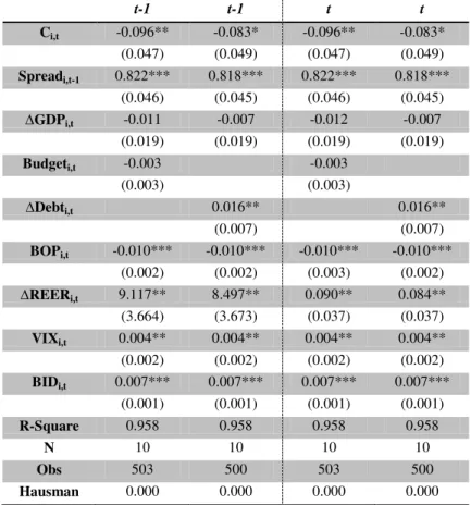
We only test the impact of the main determinants of sovereign spreads that we might call core variables (see appendix A1). In this case, we perform the Hausman's test, to verify if it is more appropriate to use fixed or random effects. Random effects are only adequate when there is a reasonable guarantee that the individual effects are not correlated with the variables taken as regressors, therefore we only apply this test when we study the impact of the core variables. When we include spreads and variation of yields in the model, the variables are correlated. The null hypothesis is the non -existence of correlation, meaning that random effects should be used. Then, when the p -values are higher than 0.10, we don't reject the null hypothesis and for p-values lower than 0.10, we consider fixed effects.
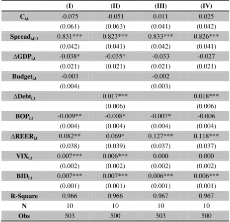
Table II - Estimation results for the determinants of 10-year yields spread: models (1) and (2)
(I) (II) (III) (IV) Ci,t -0.075 -0.051 0.011 0.025
(0.061) (0.063) (0.041) (0.042)
Spreadi,t-1 0.831*** 0.823*** 0.833*** 0.826***
(0.042) (0.041) (0.042) (0.041) ∆GDPi,t -0.038* -0.035* -0.033 -0.027
(0.021) (0.021) (0.021) (0.021)
Budgeti,t -0.003 -0.002
(0.004) (0.003)
∆Debti,t 0.017*** 0.018***
(0.006) (0.006)
BOPi,t -0.009** -0.008* -0.007* -0.006
(0.004) (0.004) (0.004) (0.004) ∆REERi,t 0.082** 0.069* 0.127*** 0.118***
(0.038) (0.039) (0.037) (0.037)
VIXi,t 0.007*** 0.006*** 0.000 0.000
(0.002) (0.002) (0.002) (0.002)
BIDi,t 0.007*** 0.007*** 0.006*** 0.006***
(0.001) (0.001) (0.001) (0.001)
R-Square 0.966 0.966 0.967 0.967
N 10 10 10 10
Obs 503 500 503 500
11
In Table II, we report the results of the estimation for the spreads of 10-year government bond yields: columns (I) and (II) report the results Model (1), and columns (III) and (IV) for Model (2).
Regarding the analysis at year t-1, we find that the spread of a given country depends significantly on the spread of the previous year. An increase of 1 percentage point (p.p.) in the spread at t-1 raises the spread in t by 0.828 p.p., on average. Public debt ratio and variation of the real effective exchange rate are also significant. An increase of 1 p.p. in the public debt ratio, increases spreads by 0.018 p.p., on average, and a positive variation of the real effective exchange rate in 1 p.p. increases spreads by 0.284 p.p. on average. The balance of payment ratio appears statistically significant in three of the four regressions, but an increase of 1 p.p. induces a small decrease in spread of 0.008 p.p. on average. The bid-ask spread has a significant impact on spreads, although of a limited magnitude. VIX and real GDP growth rate have an upward and downward effect respectively, on spreads in Model (1), 0.007 for the VIX and 0.037 p.p. for GDP, both in average. The budget balance does not come across as statistically significant.
Table III presents results for the models, including potential contagion spreads and yield variations during period t: columns (I) and (II) refer to model (3) and columns (III) and (IV) refer to model (4).
According to the results, we find that spreads in t-1 are also statistically significant. The public debt ratio and the variation of the real effective exchange rate, as above, increase spreads in 0.014 p.p. and 0.101 p.p. respectively, on average. The bid -ask spread is also statistically significant, inducing an increase in spreads of 0.008. In this case, the real GDP growth rate and the balance of payment ratio have no impact on the 10-year yield spreads. As previously, the budget balance is not significant.
12
Table III - Estimation results for the determinants of 10-year yield spreads: models (3) and (4)
(I) (II) (III) (IV) Ci,t -0.013 -0.010 -0.039 -0.026
(0.043) (0.046) (0.044) (0.047)
Spreadi,t-1 0.797*** 0.792*** 0.821*** 0.814***
(0.034) (0.033) (0.046) (0.045) ∆GDPi,t -0.016 -0.013 -0.025 -0.020
(0.021) (0.021) (0.021) (0.021)
Budgeti,t 0.000 -0.001
(0.004) (0.004)
∆Debti,t 0.012** 0.015**
(0.006) (0.006)
BOPi,t -0.003 -0.003 -0.007 -0.006
(0.005) (0.005) (0.005) (0.005) ∆REERi,t 0.091** 0.085** 0.117*** 0.111***
(0.037) (0.038) (0.039) (0.040)
VIXi,t -0.001 -0.001 0.002 0.001
(0.002) (0.002) (0.002) (0.002)
BIDi,t 0.008*** 0.008*** 0.007*** 0.007***
(0.001) (0.001) (0.001) (0.001)
R-Square 0.969 0.969 0.948 0.965
N 10 10 10 10
Obs 503 500 503 500
Note: the asterisks *, ** and *** represent significance at 10, 5 and 1% level, respectively. The values between parentheses are the standard errors. N is the number of countries included in the sample and Obs is the number of observations.
The coefficient of spreads in the previous period is positive (on average, it is 0.817), meaning that higher spreads in t-1 induce higher spreads in t. When an investor builds his expectations, he will be aware of the evolution of sovereign yields relative to German bonds. In capital markets, if there are no improvement indicators for a specific country, the spread at this time will be tightly correlated with the previous value.
Additionally, the public debt ratio has a significant impact on 10-year yield spreads, in both periods (on average, 0.016 p.p.). A worsening of the public debt ratio affects the country's probability of default and discourages investment. As a consequence, countries have to borrow abroad or from international institutions, thus deteriorating their economic situations and negatively affecting spreads. For instance, the impact of the bid-ask spreads (on average, 0.008 p.p.) is strongly significant, reflecting that investors required a greater premium for bearing a liquidity risk.
13
countries and consequently higher spreads. On the other hand, the balance of payment has a small effect on spreads and is not always present.
Concerning global risk aversion measuring by VIX, this does not affect spreads persistently, reflecting that investors do not always pay attention to global uncertainty.
Contagion
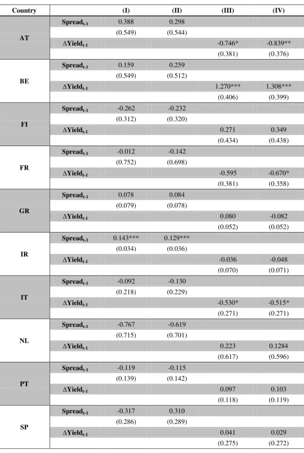
We now present the results concerning the spillover effects for the years t-1 and t in Table IV and V, respectively.
Regarding the results for spillover or contagion effects in period t-1, we can observe that there is a possible contagion from the spreads of Ireland, negatively affecting the whole country sample by 0.136 units. Looking at the change in yields, we conclude that only Belgium has an upward contagion effect on spreads, increasing overall spreads by 1.289 p.p., on average. On the other hand, a positive variation in the yields of Austria, France and Italy decrease the sample spreads (0.793 p.p., 0.670 p.p. and 0,523 p.p., respectively).
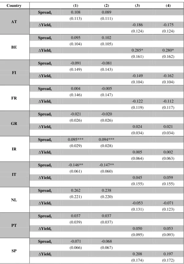
Regarding estimation results for the contagion effects in a contemporaneous fashion (Table IV), by analysing regression Models (1) and (2), the spreads of Ireland still have a significant impact, increasing spreads by 0.095 p.p. on average. On the other hand, the spread of Italy reduce the sample spreads by 0.147 p.p. In terms of specification, including the variation of the yields, only the change of yield of Belgium still has an impact, negatively affecting spreads by 0.283 p.p.
14
Table IV - Estimation results for the spillover effects in t-1
Note: the asterisks *, ** and *** represent significance at 10, 5 and 1% level, respectively.
Country (I) (II) (III) (IV)
AT
Spreadt-1 0.388 0.298
(0.549) (0.544)
∆Yieldt-1 -0.746* -0.839**
(0.381) (0.376)
BE
Spreadt-1 0.159 0.259
(0.549) (0.512)
∆Yieldt-1 1.270*** 1.308***
(0.406) (0.399)
FI
Spreadt-1 -0.262 -0.232
(0.312) (0.320)
∆Yieldt-1 0.271 0.349
(0.434) (0.438)
FR
Spreadt-1 -0.012 -0.142
(0.752) (0.698)
∆Yieldt-1 -0.595 -0.670*
(0.381) (0.358)
GR
Spreadt-1 0.078 0.084
(0.079) (0.078)
∆Yieldt-1 0.080 -0.082
(0.052) (0.052)
IR
Spreadt-1 0.143*** 0.129***
(0.034) (0.036)
∆Yieldt-1 -0.036 -0.048
(0.070) (0.071)
IT
Spreadt-1 -0.092 -0.130
(0.218) (0.229)
∆Yieldt-1 -0.530* -0.515*
(0.271) (0.271)
NL
Spreadt-1 -0.767 -0.619
(0.715) (0.701)
∆Yieldt-1 0.223 0.1284
(0.617) (0.596)
PT
Spreadt-1 -0.119 -0.115
(0.139) (0.142)
∆Yieldt-1 0.097 0.103
(0.118) (0.119)
SP
Spreadt-1 -0.317 0.310
(0.286) (0.289)
∆Yieldt-1 0.041 0.029
15
Table V - Estimation results for spillover effects, in t
Note: the asterisks *, ** and *** represent significance at 10, 5 and 1% level, respectively.
Country (1) (2) (3) (4)
AT
Spreadt 0.108 0.089
(0.113) (0.111)
∆Yieldt -0.186 -0.175
(0.124) (0.124)
BE
Spreadt 0.095 0.102
(0.104) (0.105)
∆Yieldt 0.285* 0.280*
(0.161) (0.162)
FI
Spreadt -0.091 -0.081
(0.149) (0.143)
∆Yieldt -0.149 -0.162
(0.104) (0.104)
FR
Spreadt 0.004 -0.005
(0.146) (0.147)
∆Yieldt -0.122 -0.112
(0.119) (0.117)
GR
Spreadt -0.021 -0.020
(0.026) (0.026)
∆Yieldt 0.024 0.021
(0.034) (0.034)
IR
Spreadt 0.095*** 0.094***
(0.029) (0.028)
∆Yieldt 0.005 0.002
(0.064) (0.063)
IT
Spreadt -0.146** -0.147**
(0.061) (0.060)
∆Yieldt 0.045 0.059
(0.155) (0.155)
NL
Spreadt 0.262 0.238
(0.221) (0.220)
∆Yieldt -0.053 -0.071
(0.131) (0.123)
PT
Spreadt 0.037 0.037
(0.039) (0.037)
∆Yieldt 0.050 0.053
(0.095) (0.093)
SP
Spreadt -0.071 -0.068
(0.066) (0.067)
∆Yieldt 0.208 0.197
16
4.2. Robustness
In order to check the robustness of the results, we extend our sample to three more countries outside the Euro Area: Denmark, Sweden and the United Kingdom, to test whether spillover effects can spread to non-Euro area countries for this particular assessment. We have not used variable bid-ask spread, due to the fact that it is not available for these countries. We based our analysis on the same models described above.
In Table VI, we report the results of the estimation for the spreads of 10-years government bond yields: columns (I) and (II) report estimation for Model (1), and columns (III) and (IV) for Model (2).
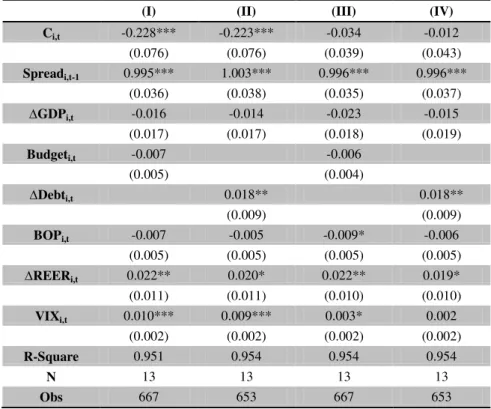
Table VI - Estimation results for the determinants of 10-years yield spreads: models (1) and (2)
(I) (II) (III) (IV) Ci,t -0.228*** -0.223*** -0.034 -0.012
(0.076) (0.076) (0.039) (0.043)
Spreadi,t-1 0.995*** 1.003*** 0.996*** 0.996***
(0.036) (0.038) (0.035) (0.037) ∆GDPi,t -0.016 -0.014 -0.023 -0.015
(0.017) (0.017) (0.018) (0.019)
Budgeti,t -0.007 -0.006
(0.005) (0.004)
∆Debti,t 0.018** 0.018**
(0.009) (0.009)
BOPi,t -0.007 -0.005 -0.009* -0.006
(0.005) (0.005) (0.005) (0.005) ∆REERi,t 0.022** 0.020* 0.022** 0.019*
(0.011) (0.011) (0.010) (0.010)
VIXi,t 0.010*** 0.009*** 0.003* 0.002
(0.002) (0.002) (0.002) (0.002)
R-Square 0.951 0.954 0.954 0.954
N 13 13 13 13
Obs 667 653 667 653
Note: the asterisks *, ** and *** represent significance at 10, 5 and 1% level, respectively. The values between parentheses are the standard errors. N is the number of countries included in the sample and Obs is the number of observations.
17
has the same impact as initial values. VIX is significant in three of four regressions, having an upward effect on spreads of 0.006 p.p., although this is a limited effect. The effect of the balance of payments ratio is only present in one equation. GDP and budget balance ratio have no impact.
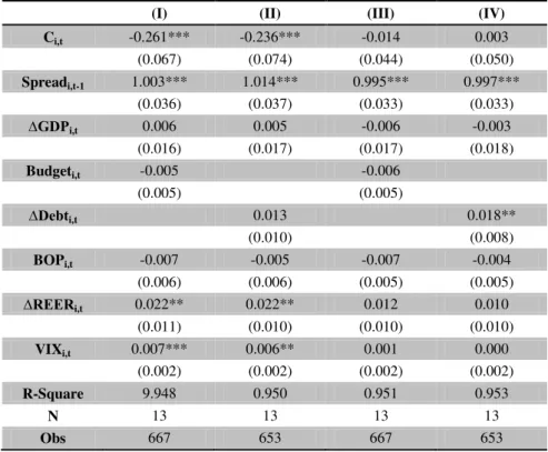
Table VII presents results for the models, including potential contagion spreads and variations of yields at period t: columns (I) and (II) refer to Model (3), and columns (III) and (IV) to Model (4).
Comparing the results, sovereign government yield spreads in the previous period continue to be significant. The public debt ratio and the variation of the real effective exchange rate push up spreads by 0.018 p.p. and 0.022 p.p. respectively, on average. VIX still has a limited effect, increasing spreads by 0.007 p.p., on average. Balance of payments, budget balance ratio and real GDP growth rate have no effect.
Table VII - Estimation results for the determinants of 10-years yield spreads: models (3) and (4)
(I) (II) (III) (IV) Ci,t -0.261*** -0.236*** -0.014 0.003
(0.067) (0.074) (0.044) (0.050)
Spreadi,t-1 1.003*** 1.014*** 0.995*** 0.997***
(0.036) (0.037) (0.033) (0.033) ∆GDPi,t 0.006 0.005 -0.006 -0.003
(0.016) (0.017) (0.017) (0.018)
Budgeti,t -0.005 -0.006
(0.005) (0.005)
∆Debti,t 0.013 0.018**
(0.010) (0.008)
BOPi,t -0.007 -0.005 -0.007 -0.004
(0.006) (0.006) (0.005) (0.005)
∆REERi,t 0.022** 0.022** 0.012 0.010
(0.011) (0.010) (0.010) (0.010)
VIXi,t 0.007*** 0.006** 0.001 0.000
(0.002) (0.002) (0.002) (0.002)
R-Square 9.948 0.950 0.951 0.953
N 13 13 13 13
Obs 667 653 667 653
Note: the asterisks *, ** and *** represent significance at 10, 5 and 1% level, respectively. The values present between parentheses are standard error. N is the number of countries included in the sample and Obs is the number of observation.
18
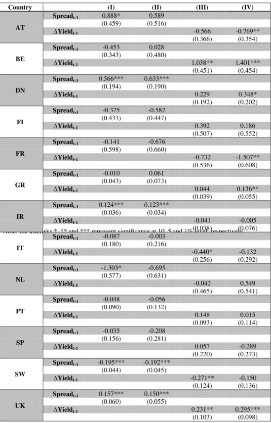
United Kingdom, have a significant impact on spreads in the country sample, increasing spreads by 0.600, 0.124 and 0.154 p.p. on average, respectively for Danish, Irish and British spreads,. On the other hand, spreads of The Netherlands and Sweden decrease the whole sample spread, respectively by 1.303 and 0.193 p.p. Looking at Models (3) and (4), the positive variation of the yields of Belgium, Denmark, Greece and United Kingdom, induce an increase spreads by 1.220, 0.348, 0.136 and 0.263 p.p. on average, respectively. The variation of the yields of Austria, France and Sweden decrease by 0.769, 1.507 and 0.271 p.p., respectively.
For the next year, period t (see appendix B2), studying Models (3) and (4), we note that the spread of Belgium, Denmark, Ireland, United Kingdom push up spreads by 0.210, 0.264, 0.062 and 0.191 p.p., respectively, on average. Regarding Swedish spreads, these reduce the whole sample spread by 0.105 p.p., on average. Looking at the remaining columns, (III) and (IV), regarding the positive variation of Belgian and Swedish yields, these induce an increase by 0.501 p.p. and 0.245 p.p, respectively, on average. On the other hand, the variation of the yields of Denmark and United Kingdom, decrease the whole sample spread by 0.163 and 0.208 p.p., respectively, both on average.
Analysis of core variables seems to confirm the idea that spreads depend significantly on the previous information. Disbelief in the capacity of a country to overcome the crisis led investors to start to give more importance to public debt. In addition, the real effective exchange rate has great importance as an indicator of the country's economic situation.
Regarding the impact of spread and variation of the yields of each country, the spread of Ireland, and the variation of the yields of Belgium, have an important effect in the whole EMU, as well as in the EU. Furthermore, countries outside the Euro Area have a significant impact on spreads, reflecting how the economic situation of all the European Union is important to stabilize the Euro Area.
4.3. Country estimation – SUR
19
approach. Although all countries belong to the European Union and some to the EMU, there are important differences in macroeconomic and fiscal fundamentals, as well as the ability of each country to tackle the sovereign debt crisis.
Thus, some countries present higher fiscal imbalances and higher public debt, which affects their credibility and they become more vulnerable to the weak economic climate. Specifically, it is more likely that the peripheral countries, such as Greece, Portugal and Ireland, are more affected by the sovereign debt crisis and will exhibit a spillover effect, rather than the core countries, such as Austria, Finland and The Netherlands.
We have estimated a system of equations to find the individual coefficients, one for each country. For this purpose, we employed the Seemingly Unrelated Regressions (SUR) model, which assumes that dependent variable and regressors may differ between equations, but that contemporary correlation exists between residuals of all equations.
For our analysis, we used a SUR model and estimate four specifications. Due to the lower significance of the budget balance, we excluded this variable from our analysis and only include the public debt ratio. The model is as follows:
(5) 𝑠𝑝𝑟𝑒𝑎𝑑𝑖,𝑡 = β0 + β1*𝑠𝑝𝑟𝑒𝑎𝑑𝑖,𝑡−1+ β2.*𝑾̅̅̅i,t + β3*vixt + β4*bidi,t + ∑𝑁𝑗=1𝛽j,t* 𝑠𝑝𝑟𝑒𝑎𝑑𝑗,𝑡−1
(6) 𝑠𝑝𝑟𝑒𝑎𝑑𝑖,𝑡 = α0 + α1*𝑠𝑝𝑟𝑒𝑎𝑑𝑖,𝑡−1+ α2.*𝑾̅̅̅i,t + α3*vixt + α4*bidi,t + ∑𝑁𝑖=1𝛼i,t* ∆𝑦𝑖𝑒𝑙𝑑𝑖,𝑡−1
(7) 𝑠𝑝𝑟𝑒𝑎𝑑𝑖,𝑡 = β0 + β1*𝑠𝑝𝑟𝑒𝑎𝑑𝑖,𝑡−1+ β2.*𝑾̅̅̅i,t + β3*vixt + β4*bidi,t + ∑𝑁𝑗=1𝛽j,t* 𝑠𝑝𝑟𝑒𝑎𝑑𝑗,𝑡
(8) 𝑠𝑝𝑟𝑒𝑎𝑑𝑖,𝑡 = α0 + α1*𝑠𝑝𝑟𝑒𝑎𝑑𝑖,𝑡−1+ α2.*𝑾̅̅̅i,t + α3*vixt + α4*bidi,t + ∑𝑁𝑗=1𝛼j,t* ∆𝑦𝑖𝑒𝑙𝑑𝑗,𝑡
From the four equations above, we create a system of ten regressions, one for each country (Austria, Belgium, Finland, France, Greece, Ireland, Italy, Netherlands, Portugal and Spain).
20
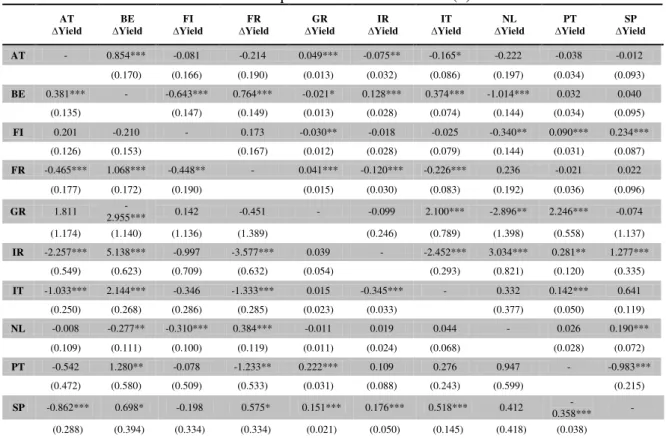
Table VIII - Spillover effect for model (5)
AT Spread BE Spread FI Spread FR Spread GR Spread IR Spread IT Spread NL Spread PT Spread SP Spread
AT 0.402 0.618** -0.231 -1.064*** 0.053 0.030 0.282** 0.580 -0.061 -0.376** (0.286) (0.292) (0.300) (0.389) (0.042) (0.023) (0.118) (0.380) (0.072) (0.156)
BE 0.002 0.649 -0.240 -0.824 0.018 0.120*** 0.114 0.460 0.099 -0.307 (0.423) (0.436) (0.456) (0.595) (0.062) (0.037) (0.178) (0.572) (0.106) (0.226)
FI 0.322* 0.373* -0.007 -1.032*** 0.041 0.005 0.125 0.458* -0.041 -0.174* (0.187) (0.207) (0.203) (0.272) (0.028) (0.018) (0.083) (0.261) (0.048) (0.103)
FR 0.213 0.186 -0.004 -0.580*** -0.014 -0.044** 0.071 0.298 0.151*** -0.116 (0.161) (0.172) (0.173) (0.223) (0.023) (0.020) (0.076) (0.217) (0.042) (0.089)
GR -4.444*** -0.873 -1.017 3.082** 0.289* -0.140 2.438*** -0.195 -1.429*** 4.649*** (1.096) (1.092) (1.005) (1.560) (0.160) (0.135) (0.697) (1.426) (0.445) (0.909)
IR 2.218** 0.243 1.464 0.125 0.434*** 1.150*** 0.312 -5.095*** -1.032*** -1.166*** (1.000) (1.029) (1.050) (1.396) (0.143) (0.109) (0.402) (1.391) (0.253) (0.525)
IT -0.455 -0.316 -1.093* 0.635 0.014 0.136** 0.259 1.920** 0.278* -0.299 (0.565) (0.552) (0.565) (0.752) (0.080) (0.057) (0.230) (0.780) (0.145) (0.299)
NL 0.446** 0.077 -0.315* -0.479** 0.068*** 0.061*** 0.197*** 0.448* -0.086* -0.340*** (0.173) (0.176) (0.180) (0.232) (0.026) (0.016) (0.074) (0.228) (0.046) (0.095)
PT -1.491*** 2.087*** 0.044 -0.833 0.287*** 0.182* 0.751** 0.196 0.091 -1.438*** (0.567) (0.732) (0.615) (0.825) (0.083) (0.094) (0.342) (0.738) (0.150) (0.337)
SP 0.481* -0.228 0.308 1.461*** 0.172*** 0.106*** -0.373*** -1.478*** -0.072 0.147 (0.285) (0.287) (0.308) (0.381) (0.041) (0.025) (0.122) (0.406) (0.072) (0.155)
Note: the asterisks *, ** and *** represent significance at 10, 5 and 1% level, respectively.
Table IX – Spillover effects model (6)
AT
∆Yield ∆YieldBE ∆YieldFI ∆YieldFR ∆YieldGR ∆YieldIR ∆YieldIT ∆YieldNL ∆YieldPT ∆YieldSP
AT 0.055 0.252 0.042 -0.496* 0.005 -0.056 0.080 0.022 0.121*** -0.026 (0.208) (0.265) (0.224) (0.263) (0.023) (0.037) (0.118) (0.295) (0.042) (0.114)
BE -0.265 -0.328 -0.202 -0.116 -0.004 0.032 0.195 0.262 0.341*** 0.083 (0.314) (0.402) (0.352) (0.393) (0.036) (0.059) (0.190) (0.441) (0.068) (0.183)
FI 0.089 0.322 -0.019 -0.641*** 0.009 -0.074** -0.072 0.333 0.069* 0.073 (0.171) (0.231) (0.195) (0.223) (0.019) (0.034) (0.108) (0.258) (0.037) (0.101)
FR 0.174 -0.010 0.026 -0.326* -0.036** -0.108*** -0.063 -0.048 0.238*** 0.131 (0.155) (0.201) (0.172) (0.194) (0.018) (0.026) (0.089) (0.215) (0.033) (0.088)
GR -3.393*** 0.500 0.068 -2.415** -0.210* 0.272 3.056*** 0.467 -1.445** 3.133*** (0.771) (0.783) (0.812) (1.087) (0.117) (0.212) (0.566) (1.171) (0.583) (0.838)
IR 0.441 0.096 0.318 0.922 0.262*** 1.006*** 0.579 -0.759 -0.625*** -2.078*** (0.749) (0.970) (0.914) (0.983) (0.089) (0.139) (0.447) (1.128) (0.191) (0.484)
IT -1.073* 0.205 -1.647*** -0.202 0.015 -0.194* -0.425 1.725** 0.670*** 0.948*** (0.567) (0.739) (0.613) (0.699) (0.065) (0.096) (0.336) (0.811) (0.122) (0.337)
NL 0.161 0.264 -0.096 -0.362* 0.037* -0.045 -0.153 0.174 0.024 0.028 (0.161) (0.212) (0.182) (0.203) (0.019) (0.029) (0.098) (0.229) (0.035) (0.092)
PT -1.083** 1.639*** 0.189 -0.857* 0.310*** 0.172** 0.849*** 1.249** -0.536*** -1.812*** (0.426) (0.579) (0.487) (0.519) (0.048) (0.070) (0.245) (0.600) (0.097) (0.253)
SP -0.271 -0.015 -0.353 0.708* 0.240*** 0.029 -0.371* 0.134 -0.115 0.119 (0.342) (0.446) (0.411) (0.423) (0.040) (0.065) (0.200) (0.510) (0.091) (0.234)
21
Table X- Spillover effects from model (7):
AT Spread BE Spread FI Spread FR Spread GR Spread IR Spread IT Spread NL Spread PT Spread SP Spread A
T - 0.446*** 0.508*** 0.301** 0.024*** -0.012 -0.047 0.077 -0.060*** -0.067***
(0.073) (0.124) (0.129) (0.009) (0.011) (0.044) (0.137) (0.017) (0.034)
BE 0.725*** - 0.203 0.542*** -0.012 0.097*** 0.309*** -0.949*** 0.045* -0.157*** (0.144) (0.185) (0.181) (0.012) (0.013) (0.061) (0.173) (0.023) (0.053)
FI 0.346*** 0.165* - -0.316** -0.034*** -0.053*** -0.177*** 0.726*** 0.083*** 0.163*** (0.099) (0.085) (0.129) (0.007) (0.012) (0.042) (0.105) (0.016) (0.032)
FR 0.200* 0.389*** -0.251** - 0.001 -0.077*** -0.054 0.418*** 0.036*** 0.048* (0.103) (0.077) (0.107) (0.007) (0.010) (0.039) (0.093) (0.014) (0.028)
G
R 3.424*** -4.314*** -1.081 1.156 - -0.121 0.843* -4.429*** 1.347*** 3.272***
(0.851) (1.106) (0.798) (1.536) (0.146) (0.475) (1.311) (0.367) (0.770)
IR -1.623** 3.401*** -1.679** -2.273*** 0.166*** - -1.952*** 6.185*** -0.194* 0.652*** (0.665) (0.391) (0.749) (0.726) (0.051) (0.219) (0.651) (0.113) (0.208)
IT -1.211*** 1.504*** -1.192*** 0.064 -0.038* -0.165*** - 2.508*** 0.081 0.425*** (0.383) (0.277) (0.337) (0.338) (0.022) (0.026) (0.340) (0.050) (0.081)
N
L 0.000 -0.332*** 0.700*** 0.420*** 0.013 0.067*** 0.178*** - -0.057*** -0.111***
(0.136) (0.095) (0.123) (0.137) (0.009) (0.012) (0.054) (0.018) (0.038)
PT -0.973*** 3.073*** 1.061*** -3.373*** 0.200*** -0.257*** -0.640*** 1.489*** - -0.614*** (0.326) (0.479) (0.407) (0.648) (0.020) (0.069) (0.220) (0.440) (0.096)
SP -2.144*** 0.983*** 0.935*** 0.193 0.191*** 0.041 0.290** 1.153*** -0.359*** - (0.281) (0.286) (0.323) (0.322) (0.016) (0.028) (0.143) (0.394) (0.035)
Note: the asterisks *, ** and *** represent significance at 10, 5 and 1% level, respectively.
Table XI – Spillover effects for model (8) AT
∆Yield ∆YieldBE ∆YieldFI ∆YieldFR ∆YieldGR ∆YieldIR ∆YieldIT ∆YieldNL ∆YieldPT ∆YieldSP
AT - 0.854*** -0.081 -0.214 0.049*** -0.075** -0.165* -0.222 -0.038 -0.012 (0.170) (0.166) (0.190) (0.013) (0.032) (0.086) (0.197) (0.034) (0.093)
BE 0.381*** - -0.643*** 0.764*** -0.021* 0.128*** 0.374*** -1.014*** 0.032 0.040 (0.135) (0.147) (0.149) (0.013) (0.028) (0.074) (0.144) (0.034) (0.095)
FI 0.201 -0.210 - 0.173 -0.030** -0.018 -0.025 -0.340** 0.090*** 0.234*** (0.126) (0.153) (0.167) (0.012) (0.028) (0.079) (0.144) (0.031) (0.087)
FR -0.465*** 1.068*** -0.448** - 0.041*** -0.120*** -0.226*** 0.236 -0.021 0.022 (0.177) (0.172) (0.190) (0.015) (0.030) (0.083) (0.192) (0.036) (0.096)
GR 1.811
-2.955*** 0.142 -0.451 - -0.099 2.100*** -2.896** 2.246*** -0.074 (1.174) (1.140) (1.136) (1.389) (0.246) (0.789) (1.398) (0.558) (1.137)
IR -2.257*** 5.138*** -0.997 -3.577*** 0.039 - -2.452*** 3.034*** 0.281** 1.277*** (0.549) (0.623) (0.709) (0.632) (0.054) (0.293) (0.821) (0.120) (0.335)
IT -1.033*** 2.144*** -0.346 -1.333*** 0.015 -0.345*** - 0.332 0.142*** 0.641 (0.250) (0.268) (0.286) (0.285) (0.023) (0.033) (0.377) (0.050) (0.119)
NL -0.008 -0.277** -0.310*** 0.384*** -0.011 0.019 0.044 - 0.026 0.190*** (0.109) (0.111) (0.100) (0.119) (0.011) (0.024) (0.068) (0.028) (0.072)
PT -0.542 1.280** -0.078 -1.233** 0.222*** 0.109 0.276 0.947 - -0.983*** (0.472) (0.580) (0.509) (0.533) (0.031) (0.088) (0.243) (0.599) (0.215)
SP -0.862*** 0.698* -0.198 0.575* 0.151*** 0.176*** 0.518*** 0.412
-0.358*** - (0.288) (0.394) (0.334) (0.334) (0.021) (0.050) (0.145) (0.418) (0.038)
22
Looking at the results, we observe that coefficients and significant variables clearly change across countries. In addition, while in the initial results, only the spread of Ireland and the variation of yields of Belgium have an important impact, now spreads and the variation of the yields of all countries have a significant effect on various countries, reflecting the spillover effect. We briefly analyse the results for each country below.
Starting with Austria, the spread is positively correlated with Belgian and Italian spreads but negatively with the spreads of France and Spain, at the period t-1. Looking at the influence of spreads in period t, the spreads of Belgium, Finland, France and Greece increase the Austrian spread, unlike the spread of Portugal and Spain which t have the opposite effect. Analysing the impact of the variation of yields in t-1, the spread of Austria is negatively correlated with the variation of the yields of France and positively with the yields variation of Portugal. At period t, the Belgian and Greek variation of yields increase the spread of Austria and the variation of the yields of Ireland and Italy decrease the Austrian spread.
Belgium's spread is only affected by the Irish spread in t-1 (increase of 0.118 p.p. whilst Irish spread increase by 1 p.p.). Looking at the impact of spreads in t of the various countries, the Belgian spread increases when the spreads of Austria, France, Ireland, Italy and Portugal increase. On the other hand, when the Dutch and Spanish spreads increase, the spread of Belgium decreases. Only the variation of the yields of Portugal in t-1 has an impact on the Belgium spread (increasing spread by 0.341 p.p.). In the period t, almost all variations of yields are significant for the spread of Belgium. The variation of the yields of Austria, France, Ireland and Italy increase spreads, unlike the variation yields of Finland, Greece and the Netherlands, which are downward relative to the Belgian spread.
23
the yields, the spread of Finland decreases when the variation of the yields of France and Ireland increase by 1 p.p. In the period t, the variation of the yields of Greece, Ireland, Italy and the Netherlands move the Finnish spread downwards and the variation of Portugal and Spain's yields pushes up the Finnish spread.
In France, the spread in t-1 is negatively affected by the Portuguese spread (French spreads increase by 0.151 p.p.) and positively affected the spreads of France itself and Ireland. Regarding the period t, all the spreads of Austria, Belgium, The Netherlands, Portugal and Spain increase the French spread. The Finnish and Irish spreads decrease the French spread. Regarding the impact of yield variation in t-1, Portugal pushes up French spreads by 0.238 p.p., unlike France, Greece and Ireland. At period t, variation of the yields of Austria, Finland, Ireland and Italy decreases the spread of France. On the other hand, Belgium and Greece's yield variations are positively correlated with the French spread.
Looking at Greece, the spreads in t-1 of France, Greece Italy and Spain increase the spread of Greece. In contrast, the spread in t-1 of Austria and Portugal push down the Greek spread. Concerning period t, in addition to the spreads of Italy and Spain, Austria and Portugal also increase the Greek spread, and Belgian and Dutch spreads are negatively correlated with Greece's spread. Regarding variation of yields in t-1, Austria, France, Greece and Portugal decrease their spread. A positive variation of Italian and Spanish yields increase the Greek spread. Looking at the period t, the variation of yields of Belgium, Ireland and Netherlands are negatively correlated with the spread of Greece, unlike the variation of the yields of Italy and Portugal.
24
For Italy, in t-1, the spreads of Ireland, Netherlands and Portugal increase the Italian spread, unlike the spread of Finland. For the period t, the spreads of Belgium, Netherlands and Spain are positively correlated with the Italian spread. On the other hand, an increase in the spreads of Austria, Finland, Greece and Ireland decreases the spread of Italy. Regarding the results of the influence of the yield variation in t-1, the variation of the yields of Netherlands, Portugal and Spain are positively correlated with the Italian spread, as opposed to the Austrian, Finnish and Irish variation yields. The variation of the yields in t of Belgium and Portugal increase the Italian spread. The changes in the yields of Austria, France and Ireland in t affect Italy's spread negatively.
Looking at the results for The Netherlands, the spillover effect of the spreads of each country has more impact than the influence of yield variation. Concerning the period t-1, except for Belgium spreads, all spreads have an impact on the Dutch spread. The spreads of Finland, France, Portugal and Spain decrease the spread of The Netherlands, as opposed to the remaining countries. At period t, in addition to spreads of Portugal and Spain pushing down the Dutch spreads, the spread of Belgium significantly does the same. The spreads in t of France, Finland, Ireland and Italy are positively correlated. The variation of the yields of Greece and France in t-1 decrease and increase the spread of The Netherlands, respectively. The Belgian and Finnish yield variation in t are negatively correlated with the Dutch spread, yet on the other hand, a positive variation in the yields of France and Spain induces an increase in the spread of The Netherlands.
25
Finally, in terms of the results for Spain, an increase in spreads, in t-1, of Austria, France, Greece and Ireland, induced an increase in Spanish spreads, on the other hand, an increase in Italian and Dutch spreads has the opposite effect. For the period t, the spreads of Belgium, Finland, Greece, Italy and Netherlands increase the spread of Spain and the spreads of Austria and Portugal are negatively correlated with the Spanish spread. Regarding the variation of the yields of France and Greece in t-1, when they increase by 1 p.p., Spanish spreads also increase, in contrast, when there is a positive variation in Italian yields, the spread of Spain decreases. At period t, yield variations of Belgium, France, Greece, Ireland and Italy are positively correlated with the Spanish spread, as opposed to those of Austria and Portugal.
As expected, the spillover effect from Greece, Ireland and Portugal tends to be higher than in other countries. In addition, Belgium, Italy, Netherlands and Spain also have a large influence on the spreads of the other countries, due to the deterioration of their fiscal and macroeconomic fundamentals, namely higher public debt. On the other hand, Austria, Finland and France are also affected, but they have a positive impact on almost all countries and still maintain credibility in their economies. After carrying out the individual analysis, the presence of contagion between the EMU countries is confirmed.
Observing the results for potential contagion, including those of Denmark, Sweden and the United Kingdom, in Appendix E, Tables E1, E2, E3 and E4, we note that spreads and the variation of the yields of those countries have a big impact on the spreads of the other countries, supporting the idea that the stability of EMU countries is affected by countries outside the Euro area.
5. Conclusion
26
Our empirical findings indicate that there is a spillover effect between the EMU countries that can spread throughout EU countries. The EMU countries more affected by the three risks factors mentioned at the beginning of this work, namely: international, credit, and liquidity risk are more vulnerable to possible contagion across countries. These factors have a negative impact on the credibility of these countries and drive investors away from them. Therefore, the determinants of government yield spreads involved in the three risks factors, real effective exchange rate, VIX and bid-ask spread, operate as a transmission mechanism of sovereign debt crisis and enable contagion. Finally, public debt ratio is also statistically significant in explaining spreads relative to macroeconomic and fiscal fundamentals, which shows the important key role it performs in the sovereign debt crisis.
References
Afonso, A., Arghyrou, M. and Kontonikas, A. (2012). “The determinants of sovereign bond yield spreads in the EMU”, Department of Economics, ISEG-UTL, Working Paper 36/2012/DE/UECE.
Arghyrou, M. and Kontonikas, A. (2011). “The EMU sovereign-debt crisis: Fundamentals, expectations and contagion”, European Commission, Economic Papers 436.
Barrios, S., Iversen, P., Lewandowska, M., and Setzer, R. (2009). “Determinants of intra-euro-area government bond spreads during the financial crisis”, European Commission, Economic Paper 388.
Bernoth, A. and Erdogan, B. (2010). “Sovereign bond yield spreads: A time-varying coefficient approach”, Department of Business Administration and Economics, European University Frankfurt (Oder), Discussion paper 289.
Bernoth, K., von Hagen, J., Schuknecht, L. (2004). “Sovereign risk premia in the European government bond market”. ECB Working Paper 369.
Caceres, C., Guzzo, V. and Segoviano, M. (2010). “Sovereign Spreads: Global Risk Aversion, Contagion or Fundamentals?”, IMF Working Paper 10/120.
27
Favero, C., Pagano, M., von Thadden, E.-L. (2010). “How Does Liquidity Affect Government Bond Yields?”. Journal of Financial and Quantitative Analysis, 45, 107-134.
Gerlach, S., Schulz, A., Wolff, G. (2010). “Banking and Sovereign Risk in the Euro Area”. CEPRF Discussion Paper No. 7833.
Geyer, A., Kossmeier, S., Pichler, S. (2003). “Measuring Systematic Risk in EMU Government Yield Spreads”. Review of Finance, 8, 171-197.
Giordano, L., Linciano, N. and Soccorso, P. (2012). “The determinants of government yield spreads in the euro area”, Commissione Nazionale Per Le Società e La Borsa, Working Paper 71.
Jankowitsch, R., Mösenbacher, H., Picheler, S. (2006). “Measuring the Liquidity Impact on EMU government bond prices”. European Journal of Finance, 12, 153-169. Kilponen, J., Laakkonen, H. and Vilmunen, J. (2012). “Sovereign risk, European crisis
resolution policies and bond yields”, Bank of Finland Research Discussion Papers 22.
Missio, S., and Watzja, S. (2011). “Financial Contagion and the European Debt Crisi”. Ludwig-Maximilian-University of Munich.
Pagano, M. and von Thadden, E.L. (2004). “The European bond market under EMU”, Oxford Review of Economic Policy, 20, 531-554.
Pericoli, M. and Sbracia, M (2011). “A Primer on Financial Contagion”. Temi di discussion del Servizio Studi, Banca d’Italia, Working Paper 407.
Schuknecht, L., von Hagen, J., Wolswijk, G. (2010). “Government bond risk premiums in the EU revisited: The impact of the financial crisis”. ECB Working Paper 1152. Sgherri, S. and Zoli, E. (2009). “Euro area sovereign risk during the crisis”, IMF
39
Appendix A – Core variables:
Table A1 - Random effects analysis for 10 countries
t-1 t-1 t t
Ci,t -0.096** -0.083* -0.096** -0.083*
(0.047) (0.049) (0.047) (0.049)
Spreadi,t-1 0.822*** 0.818*** 0.822*** 0.818***
(0.046) (0.045) (0.046) (0.045) ∆GDPi,t -0.011 -0.007 -0.012 -0.007
(0.019) (0.019) (0.019) (0.019)
Budgeti,t -0.003 -0.003
(0.003) (0.003)
∆Debti,t 0.016** 0.016**
(0.007) (0.007)
BOPi,t -0.010*** -0.010*** -0.010*** -0.010***
(0.002) (0.002) (0.003) (0.002) ∆REERi,t 9.117** 8.497** 0.090** 0.084**
(3.664) (3.673) (0.037) (0.037)
VIXi,t 0.004** 0.004** 0.004** 0.004**
(0.002) (0.002) (0.002) (0.002)
BIDi,t 0.007*** 0.007*** 0.007*** 0.007***
(0.001) (0.001) (0.001) (0.001)
R-Square 0.958 0.958 0.958 0.958
N 10 10 10 10
Obs 503 500 503 500
29
Appendix B – Spillover effects for EU countries:
Table B1 - Spillover effects in t-1 for 13 countries
Note: the asterisks *, ** and *** represent significance at 10, 5 and 1% level, respectively.
Note: the asterisks *, ** and *** represent significance at 10, 5 and 1% level, respectively.
Country (I) (II) (III) (IV)
AT
Spreadt-1 0.888* 0.589
(0.459) (0.516)
∆Yieldt-1 -0.566 -0.769**
(0.366) (0.354)
BE
Spreadt-1 -0.453 0.028
(0.343) (0.480)
∆Yieldt-1 1.038** 1.401***
(0.451) (0.454)
DN
Spreadt-1 0.566*** 0.633***
(0.194) (0.190)
∆Yieldt-1 0.229 0.348*
(0.192) (0.202)
FI
Spreadt-1 -0.375 -0.582
(0.433) (0.447)
∆Yieldt-1 0.392 0.186
(0.507) (0.552)
FR
Spreadt-1 -0.141 -0.676
(0.598) (0.660)
∆Yieldt-1 -0.732 -1.507**
(0.536) (0.608)
GR
Spreadt-1 -0.010 0.061
(0.043) (0.073)
∆Yieldt-1 0.044 0.136**
(0.039) (0.055)
IR
Spreadt-1 0.124*** 0.123***
(0.036) (0.034)
∆Yieldt-1 -0.041 -0.005
(0.038) (0.076)
IT
Spreadt-1 -0.087 -0.003
(0.180) (0.216)
∆Yieldt-1 -0.440* -0.132
(0.256) (0.292)
NL
Spreadt-1 -1.303* -0.695
(0.577) (0.631)
∆Yieldt-1 -0.042 0.549
(0.465) (0.541)
PT
Spreadt-1 -0.048 -0.056
(0.090) (0.132)
∆Yieldt-1 0.148 0.015
(0.093) (0.114)
SP
Spreadt-1 -0.035 -0.208
(0.156) (0.281)
∆Yieldt-1 0.057 -0.289
(0.220) (0.273)
SW
Spreadt-1 -0.195*** -0.192***
(0.044) (0.045)
∆Yieldt-1 -0.271** -0.150
(0.124) (0.136)
UK
Spreadt-1 0.157*** 0.150***
(0.060) (0.055)
∆Yieldt-1 0.231** 0.295***
30
Table B2 - Spillover effects in t for 13 countries
Note: the asterisks *, ** and *** represent significance at 10, 5 and 1% level, respectively.
Country (I) (II) (III) (IV)
AT
Spreadt -0.106 -0.122
(0.117) (0.111)
∆Yieldt -0.074 -0.064
(0.114) (0.112)
BE
Spreadt 0.212* 0.208*
(0.114) (0.115)
∆Yieldt 0.506*** 0.495***
(0.172) (0.174)
DN
Spreadt 0.195 0.264*
(0.152) (0.144)
∆Yieldt -0.172 -0.163*
(0.105) (0.097)
FI
Spreadt 0.015 -0.003
(0.143) (0.141)
∆Yieldt 0.038 0.018
(0.101) (0.090)
FR
Spreadt -0.015 -0.028
(0.132) (0.132)
∆Yieldt 0.117 0.110
(0.131) (0.131)
GR
Spreadt -0.006 -0.006
(0.027) (0.028)
∆Yieldt 0.053 0.045
(0.036) (0.036)
IR
Spreadt 0.062 0.062**
(0.027) (0.027)
∆Yieldt 0.038 0.028
(0.064) (0.063)
IT
Spreadt -0.062 -0.058
(0.063) (0.067)
∆Yieldt -0.032 -0.048
(0.152) (0.158)
NL
Spreadt -0.067 -0.065
(0.200) (0.197)
∆Yieldt 0.019 -0.018
(0.130) (0.123)
PT
Spreadt 0.001 0.002
(0.048) (0.048)
∆Yieldt -0.088 -0.053
(0.095) (0.095)
SP
Spreadt -0.034 -0.037
(0.057) (0.063)
∆Yieldt 0.041 0.072
(0.182) (0.190)
SW
Spreadt -0.107** -0.102**
(0.048) (0.050)
∆Yieldt -0.255*** -0.234***
(0.084) (0.081)
UK
Spreadt 0.196*** 0.185***
(0.047) (0.050)
∆Yieldt -0.204*** -0.211***
31
Appendix C - SUR baseline results, including debt:
Table C1 – Results for the core variables of model (5)
Ci,t Spreadt-1 ∆GDPi,t ∆Debti,t BOPi,t ∆REERi,t BIDi,t VIXi,t R-Square Obs
AT -0.124 0.397 -0.009 0.000 0.004** 5.768** 0.001 0.006*** 0.952 51
(0.134) (0.285) (0.011) (0.002) (0.002) (2.372) (0.001) (0.002)
BE -0.138 0.663 0.002 0.001 -0.003 6.704* -0.002 0.010*** 0.965 51
(0.178) (0.435) (0.023) (0.002) (0.002) (3.509) (0.003) (0.003)
FI 0.002 -0.007 -0.013*** -0.002 0.001 0.030** 0.001 0.006*** 0.935 51
(0.071) (0.203) (0.005) (0.002) (0.002) (0.014) (0.001) (0.001)
FR 0.549*** - -0.580*** -0.003 0.008*** -0.003 0.038*** 0.000 0.004*** 0.984 51
(0.100) (0.223) (0.010) (0.002) (0.004) (0.013) (0.001) (0.001)
GR 0.503 0.289* 0.021 -0.010 0.000 0.019 0.017*** 0.013** 0.993 42
(1.170) (0.160) (0.033) (0.012) (0.006) (0.083) (0.001) (0.006)
IR -0.269 1.150*** 0.019 0.002 0.008 0.182*** 0.009*** 0.008 0.989 51
(0.192) (0.109) (0.014) (0.005) (0.012) (0.061) (0.001) (0.007)
IT -0.258 0.259 -0.015 0.002 0.008 0.048 0.002*** 0.015*** 0.987 51
(0.733) (0.230) (0.029) (0.007) (0.012) (0.051) (0.001) (0.004)
NL 0.073 0.448* -0.029*** -0.003** -0.001 0.041*** 0.000 0.005*** 0.940 51
(0.068) (0.228) (0.007) (0.001) (0.002) (0.014) (0.001) (0.001)
PT -0.270 0.091 0.038 0.000 0.005 0.111 0.011*** 0.009** 0.998 51
(0.344) (0.150) (0.024) (0.006) (0.008) (0.068) (0.001) (0.004)
SP -0.169 0.147 -0.032 0.002 -0.005 0.104*** 0.009*** 0.005** 0.997 51
(0.145) (0.155) (0.025) (0.003) (0.006) (0.030) (0.001) (0.002)
32
Table C2 - Results for the core variables of model (6)
Ci,t Spreadt-1 ∆GDPi,t ∆Debti,t BOPi,t ∆REERi,t BIDi,t VIXi,t R-Square Obs
AT -0.033 0.763*** -0.015 0.000 0.004* 0.098*** 0.001 0.002 0.965 51
(0.132) (0.056) (0.011) (0.002) (0.002) (0.021) (0.001) (0.001)
BE -0.140 0.618*** 0.025* 0.001 -0.001 0.135*** 0.005*** 0.005** 0.973 51
(0.095) (0.064) (0.015) (0.001) (0.002) (0.032) (0.002) (0.002)
FI -0.104 0.675***
-0.017*** 0.002 0.001 0.036** 0.001 0.004** 0.932 51
(0.065) (0.064) (0.006) (0.001) (0.002) (0.015) (0.001) (0.001)
FR -0.148** 0.851*** 0.012 0.002** -0.002 0.077*** -0.001 0.002* 0.981 51
(0.058) (0.044) (0.009) (0.001) (0.004) (0.014) (0.001) (0.001)
GR -1.095** 0.618*** -0.055** 0.011** 0.001 0.156** 0.020*** -0.001 0.995 42
(0.502) (0.058) (0.025) (0.005) (0.005) (0.064) (0.002) (0.004)
IR -0.601*** 0.392*** 0.017 0.021*** 0.026** (0.163)*** 0.009*** 0.001 0.991 51
(0.140) (0.059) (0.014) (0.004) (0.011) (0.060) (0.002) (0.005)
IT 1.073* 0.881*** 0.002 -0.011** 0.009 0.152*** -0.001 0.006* 0.982 51
(0.552) (0.050) (0.030) (0.005) (0.011) (0.055) (0.001) (0.003)
NL -0.106* 0.700*** -0.018** 0.002* 0.001 0.064*** 0.001 0.002* 0.933 51
(0.063) (0.065) (0.008) (0.001) (0.002) (0.017) (0.001) (0.001)
PT -0.327** 0.697*** 0.039* 0.003 -0.002 0.037 0.011*** 0.008*** 0.999 51
(0.134) (0.020) (0.021) (0.002) (0.007) (0.058) (0.000) (0.008)
SP -0.284* 0.807*** 0.045 0.003 -0.006 0.180*** 0.009*** 0.001 0.995 51
(0.172) (0.034) (0.033) (0.003) (0.007) (0.040) (0.001) (0.002)