EMERGING MARKETS YIELD CURVE DYNAMICS
Candidate: Rubens Hossamu Morita
1Advisor: Rodrigo De Losso da Silveira Bueno
GETULIO VARGAS FUNDATION
SÃO PAULO ECONOMIC SCHOOL
November 22, 2007
1I would like to thank Denísio Liberali, Luis Cláudio Barcelos, and Fernando Siqueira
Abstract
This work extendes Diebold, Li and Yue’s (2006) about global yield curve and pro-poses to extend the study by including emerging countries. The perception of emerg-ing market su¤ers in‡uence of external factors or global factors, is the main argument of this work. We expect to obtain stylized facts.that obey similar pattern found by those authors. The results indicate the existence of global level and global slope fac-tors. These factors represent an important fraction in the bond yield determination and show a decreasing trend of the global level factor low in‡uence of global slope factor in these countries when they are compared with developed countries.
1
Introduction
The term structure of interest rate stands for the relationship between bond yields and their redemption date, or maturity. Macroeconomic variables and other latent factors determine such relationship and therefore have been studied for a considerable time by academics. The term structure analysis provides a method to extract infor-mation from the interaction between those variables, and to forecast how changes in the economic environment may a¤ect the shape of the term structure.
The focus of most studies about yield curve has been on the single-country case using idiosyncratic macroeconomic factors to model the yield. For example, the framework used by Ang and Piazzesi (2003) is the a¢ne models.
The assumption that latent factors generates the yield curve has widely driven the literature on term structure, and some instances are Litterman and Scheinkman (1991); Balduzzi, Das, and Sundaram (1996); Bliss (1997a); and Dai and Singleton (2000). Such factors are usually interpreted as level, slope and curvature, according to Andersen and Lund (1997), Diebold and Li (2006), and Diebold, Rudebusch and Aruoba (2006).
Because the interactions in the global bond markets are very complex, the need to study the relationship in a cross-country environment is enormous. Notwithstanding, it is uncommon to focus on cross-country market, and the exception is Diebold, Li and Yue (2006), who determine the existence of common global yield factors. Speci…cally, they show the dynamics of cross-country bond interactions using a few countries from OCDE. Their paper follows Nelson and Siegel’s (1987) framework, which was extended by Diebold and Li (2006), in such a way that the model is a hierarchical dynamic setting for the countries’ yield curve, which depend both on idiosyncratic factors and global factors. Despite the fact the model follows a di¤erent framework from others that are in the global environment, such as Solnik (1974) and Thomas and Wickens (1993), it shares similar concerns. Then, Diebold, Li and Yue (2006) determine how the factors are interrelated between each other.
Another important concern is how to measure the global factors. Observed macro-economic global factors are inadequate to explain the yield curve because each coun-try’s macroeconomics measurement methodology may be quite di¤erent. On the other hand, any attempt to extract those variables using, for example, principal components analysis is potentially inferior than more structured methodologies that take into account latent variables as the Kalman Filter. Hence, the correct mea-surement of existing, but latent, global factors is crucial quantify, for example, the country vulnerability or the market integration.
process has brought a new dimension up in the world’s bond market. Currently the U.S. bonds correspond to less than 50% of all private and governmental bonds issued around the world. At the same time, the sovereign bonds of emerging markets have increased steadily since their debts has been renegotiated. In search for superior returns and with a long run horizon for investments, pension funds and mutual investment funds has absorbed these bonds. However, in spite of such a growing importance, emerging markets bonds studies have been neglected by the literature. Then, this work comes to bridge such gaps. It uses Diebold, Li and Yue’s (2006) framework to extract global factors related to sovereign bonds from emerging market. The possibility that emerging markets react to global factors is great, but it is neither clear nor well established by any other paper to the best of our knowledge. Therefore, our contribution is to determine whether there exist such global factors, how they explain the term structure dynamics of each country, and compare the results with other existing studies.
The paper is organized as follows. Section (2) presents the theoretical model. Section (4) show the main results, and Section (5) concludes.
2
Theoretical Model
2.1
The Nelson-Siegel’s and Diebold-Li’s Models
Milton Friedman’s claim regarding to the need of a parsimonious model to describe the yield curve has inspired Nelson and Siegel (1987), henceforth NS, to …rst propose a model for describing that curve. Friedman says: “Students of statistical demand functions might …nd it more productive to examine how the whole term structure of yield can be described more compactly by a few parameters.” Then, NS follows Friedman’s advice and come up with a simple and parsimonious model, but su¢-ciently ‡exible to represent the most common shapes associated with the yield curve: monotonically increasing, humped, and S shaped.
Typical yield curve shapes are generated by a class of functions associated with the solutions of di¤erential and di¤erence equations. For instance, let dt(m) denote the price ofm periodsdiscounted bound, i.e,dt(m)is the present value at timetof
$1receivablem periods from today. Letyt(m)denote the continuously compounded zero-coupon nominal yield to maturity, or spot rate. From the yield curve it is possible to obtain the discount curve:
The continuously compounded spot rate is the single rate of return applied until the maturity ofm years from today:
yt(m) =
ln(d(m))
m
Another important concept is theforward rate, ft;which measures the prevalent rate in each point in the future. The forward rate average de…nes the yield to maturity as follows:
yt(m) =
1
m
Z m
0
ft(x)dx; (2) where ft(x) denotes the forward rate curve as a function of the maturitie m and
t= 1;2; :::; T.
Hence, from the discount curve (1) and (2) it is possible to obtain the instanta-neous (nominal) forward rate curve:
ft(m) =
d0
t(m)
dt(m)
= [yt(m) +m y
0
t(m)]: (3) The heuristic motivation to investigate how the shapes are comes from the expec-tation theory on the term structure of interest rates. If the spot rates are generated as solutions of a di¤erential equation, then the solution of this equation will be also a forward rates. For instance, NS considered a second order di¤erential equation to describe the movements of the yield curve, and hence, with the assumption of real and unequal roots, the solution will be the forward rate:
ft(m) =b0;t+b1;t e 1;tm+b2;t e 2;tm; (4) where
1;t and 2;t are time factor loadings associated with the equations;
b0;t,b1;t, andb2;t are coe¢cients to be determined based on initial conditions; and
t= 1; :::; T.
Hence, the equation (4) gives us a family of forward rate curves whose shapes depend on the values of b1;t, and b2;t, whileb0;t is the asymptote.
There are some problems associated with that function. Depending on the para-meters 1 and 2, there is more than one value for bs that generate similar curves,
such that the bs are not unique. Another problem appears when the convergence
In order to overcome such di¢culties, NS suggested a more parsimonious model. It generates the same range of shapes of previous speci…cation, but di¤ers from equation (4) by having identical roots as equation (5) shows:
ft(m) = b0;t+b1;t e tm+b2;t tm e tm : (5) The model may be viewed as a constant plus a Laguerre function, that is a poly-nomial times an exponential decay term, which belongs to a mathematical class of approximating functions1. Then, the solution for the yield as a function of maturity may be found by solving equation (2):
yt(m) =b0;t+ (b1;t+b2;t)
1 e tm
tm
b2;t e tm: (6) for t= 1;2; :::; T.
The limiting path of y(m); when m increases, is its asymptote b0;t; and, when
m is small, the limit is (b0;t +b1;t). Di¤erent shapes can be drawn by varying the parameters and bs. If t = 1, b0;t = 1 ,(b0;t+b1;t) = 0; and b2;t =a where a 2Z; then equation (6) becomes:
yt(m) = 1
(1 a) (1 e m)
m a e
m
Considering a given periodtand by varying the parametera between 6and 12,
representing the curves from below to above, the …gure shows the possible shapes that one can draw:
1Please, see details in Abramowitz, Milton and Irene (1965, ch. 22), and Whittaker and Watson
Figure 1: Yield Curve Shapes
NS’s model creates two shortcomings. The …rst is conceptual and claims that it is di¢cult to give intuitive interpretations for the factors. The second is operational and says it is hard to estimate precisely the factors, because some multicolinear-ity can emerge. Then, Diebold and Li’s (2006), henceforth DL, proposes another factorization:
yt(m) = 0;t+ 1;t
1 e tm
tm
+ 2;t
"
1 e tm
tm
e tm
#
: (7)
The main distinction is the way they factorize the equation (6). The original NS model matches the DL’s when 0;t = b0;t; 1;t = b1;t +b2;t , 2;t = b2;t. DL’s factorization is preferable to NS’s because both (1 e tm)
tm and e
tm have similar
decreasing shapes, and, if b1;t and b2;t are interpreted as factors, their respective loadings, (1 e tm)
tm and e
tm, would be very similar.
The factor loadings 1, (1 e tm)
tm and e
tm, can be easily extracted using the
strength of long, medium and short term components of the forward rate or of the yield curve.
The parameter is related to the exponential decay rate. Small values of produce slow decay, and …t well long term maturities; by contrast, large values of produce fast decay and …t better curves that have short term maturities. DL choose a constant value for , in such a way that to maximize the curvature loading. Since, it is usually observed that maturity …nds the maximum point between 2 and 3 years2, DL use the average between these two maturities and set = 0:0609, corresponding
to 30 months.
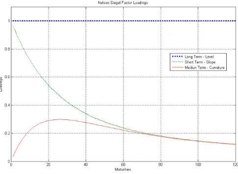
The shape of the factor loadings, 1, (1 e
m)
m , and
(1 e m)
m e
m are
illus-trated in …gure (2). As mentioned before, the factor corresponding to 0;t represents the long term, the one corresponding 2;t represents the medium term, and the last one corrsponding to 1;t represents the short term.
Figure 2: Nelson-Siegel Factor Loadings
3
The Global Model
Last section showed that studies of the U.S. closed-economy environment using a generalized DL model …t well the dynamics of the yield curve. Now, in this section the model will be extended to a multi-country environment, following Diebold, Li and Yue (2006), henceforth DLY.
Using the DL factorization of the NS yield curve for a single country and indexing the parameters to represent a speci…c country, the model is:
yi;t(m) = li;t+si;t
1 e i;tm
i;tm
+ci;t
"
1 e i;tm
i;tm
e i;tm
#
+"i;t(m); (8) where
yi;t(m)is the continously-compounded zero-coupon nominal yield of a bond ma-turingm periods ahead, in country iat period t;
i= 1;2; : : : ; N; and t = 1;2; : : : ; T;
"i;t(m)represents a disturbance with variance 2i(m):
The coe¢cients are interpreted as latent factors. They are the level, the slope, and the curvature, denoted, respectively, byl,s, and c.
The previous model was simpli…ed by DL as shown in equation (9). The …rst simpli…cation makes i;t constant across countries and time. The authors argue there is a tiny loss of generality from doing that, since determines the maturity at which the curvature loading reaches the maximum. The second simpli…cation makes ci;t = 0 for all t and i. The argument for doing that comes from the fact that missing data makes the estimated curve be considerably imprecise at very short and/or very long maturities. They also allege that the curvature is not associated with macoreconomic fundamentals, as level is connected to in‡ation and slope is connected with GDP or capacity of utilization. Hence, the model can be written as:
yi;t(m) =li;t+si;t
1 e m
m +"i;t(m): (9)
In Diebold, Rudebusch and Aruoba (2006), the single-country version was ex-pressed in terms of a space-state framework, such that equation (9) represents the space equation, and the time varying parameterslitandsit, which follow a …rst-order diagonal autoregression vector, represents the state equations.
From the single-country model, one may adapt it to an N-country approach,
Yt(m) =Lt+St
1 e m
m +vt(m) (10)
where
Yt(m)is a theoretical global yield;
Lt is the global level; and
St is the global slope.
These latent global factors are common to every country. It is postulated that the global yield factors follow a …rst-order VAR model as follows:
Lt
St =
11 12
21 22
Lt 1
St 1 +
Ul t Us t (11) where
Utn is the structural disturbance n=l; s;and
E UtnUn
0
t0 =
( n)2, if t=t0 and
n =n0
0, otherwise .
Then the model decomposes the country-speci…c level (slope) into a global level (slope) and some idiosyncratic fator,"ni;t:
li;t = li+ l
iLt+"li;t; (12a)
si;t = si + s
iSt+"si;t; (12b) for every i= 1;2; : : : ; N:
Equation (11) assumed that global common factor followed a …rst-order V AR.
Here it will be allowed that the country idiosyncratic factors share the same charac-teristic.
"li;t
"si;t
= i;11 i;12
i;21 i;22
"li;t 1
"si;t 1
+ u
l it
usit
(13)
Where
unit is the disturbancen =l; s; and
E unitun
0
it0 =
( n
2)2; if i=i 0 and
t=t0
0; otherwise
2 6 6 6 6 6 6 4
y1t(m1)
y1t(m2)
:: :: yN t(mJ 1)
yN t(mJ)
3 7 7 7 7 7 7 5
J N x1
=A 2 6 6 6 6 6 6 4 l 1 s 1 :: :: l N s N 3 7 7 7 7 7 7 5
2J x1
+C (14a)
C =B Lt St 2 1
+A 2 6 6 6 6 6 6 4 "l 1t "s 1t :: :: "l N t "s N t 3 7 7 7 7 7 7 5
2J 1
(14b)
Where, N is the numbers of countries,J is the number of maturities and, A ,B
ndC are:
A= 0 B B B B B B @
1 1 e m1
m1 0 :: 0 0
1 1 e m2
m2 0 :: 0 0
:: :: :: :: :: ::
0 0 :: :: 1 1 e mJ 1
mJ 1
0 0 :: :: 1 1 e mJ
mJ 1 C C C C C C A
J N 2:J
(14c) B = 0 B B B B B B B B B B @ l 1 s
1 1 e
m1
m1
l
1
s
1 1 e
m2 m2 ::: ::: ::: ::: l N s N 1 e
mJ 1
mJ 1 l N s N 1 e mJ mJ 1 C C C C C C C C C C A
J N 2
(14d) C = 2 6 6 6 6 6 6 4
1t(m1) 1t(m2)
:: ::
N t(mJ 1)
N t(mJ)
3 7 7 7 7 7 7 5
J N 1
It is important to note that the global common factor, 0
sand the factor loading,
1 e mJ 1
mJ 1 are not separately identi…ed
3. Because of this it will be considered
that n
BR is positive, that is n
BR>0and n=l; s; and because of the magnitudes of global factors and factor loadings the innovations to global factors have unit standard deviation, that is, n = 1; n=l,s4:
3In equation (14d)
3.1
Econometric Estrategy
The estimation method in a multi-country enviroment can be done using the equation(14a,and 14b). The state-space can be estimated by Kalman Filter, and fully-e¢cient Gaussian
maximum likelihood dynamics estimates are obtained. In the single-country situa-tion, to estimate the latent factors using Kalman Filter framework is relatively easy, because the number of parameters is small. In a multi-country situation, however, one-step maximum likelihood is di¢cult to implement, due to the large number of parameters for estimate. Hence, DLY propose a convenient multi-step estimation method.
The …rst step is to obtain the latent factors (level and slope) for each country. The second step is to use estimates previously obtained and use equations(11,12a,12b, and 13) to extract the global factors.
3.1.1 Single Country Estimation
In equation (6) are able to see that is time varying, following the original NS model. So, the parameters (li;t; si;t and t) are able to estimate using nonlinear least square for each month t. However DL use di¤erent strategy. They …x the parameter at
a speci…c value. In the …rst moment they compute two regressors (factor loadings5) for many maturities, and they use ordinary least square in these cross-section data to estimate the parameters (li;t and si;t ), for each month. Hence, there are two parameters for each month, which are li;t and si;t for speci…c country i and speci…c date t:
Furthermore, DL’s model can be represented as a space state system, where the latent factors represent the state and the main formula the space. This method is used to estimate the parameters (lit and sit ) can be obtained using the state-space system, following Diebold-Rudebush-Aruoba(2006). In general, the state- space-state system is a powerful framework for estimation of dynamic models, because it is possible to apply the Kalman Filter that provides maximum-likelihood estimates of factors. In the equation (9),li;tand si;t follow a vector autoregressive6 process of …rst order, and because of this, the model became a state-space system. The transition equation or the state equation, which governs the dynamics of state vector7, is:
5The factor loadings are not stochastic and they are obtained using 1 e mN
mN for slope factor
and level is1for all maturities, as the …gure(2).
6It will be maintain theV AR(1) assumption for transparency and parsimony.
7The initial values of coe¢cients to proceed this estimation will be obtained in Diebold-Li (2006)
method using unconditional V AR(1) in level and slope factors. The V AR(1) diagonal principal
li;t i;l
si;t i;s
= a11 a12
a21 a22
li;t 1 i;l
si;t 1 i;s
+ ni;t(l)
ni;t(s)
(15)
Where
i= 1; : : : N is the speci…c country, and t= 1; :::; T.
The set of yield curves equations with a set ofN yields and the three unobservable
factors, is: 0 B B B B @
yi;t(m1)
yi;t(m2)
: : yi;t(mN)
1 C C C C A= 0 B B B B B @
1 1 e m1
m1
1 1 e m2
m2
: : : :
1 1 e mN
mN 1 C C C C C A li;t
si;t +
0 B B B B @
i;t(m1)
i;t(m2)
: :
i;t(mN)
1 C C C C A (16)
In the vector/matrix notation, the state-space system is:
(xi;t i) =A(xi;t 1 i) + i;t (17a)
yi;t = xi;t+ i;t (17b)
The Kalman Filter is used to provide the least square estimators of state vectors, and it requires that the white noise transition and measurement disturbance be orthogonal to each other and to initial states.
i;t i;t
W N 0
0 ;
Q 0
0 H (18)
E(f0 0
i;t) = 0 (19)
E(f0 0
i;t) = 0 (20)
The analysis assumes that the H matrix is diagonal and this assumption implies
that the deviations of yields of various maturities from yield curve are uncorrelated, that is quite standard. TheQmatrix is not assumed to be diagonal or unrestricted,
and this allows that the shocks of the two latent factors be correlated.
The Kalman …lter single country factor extraction provides similar results than DL method, and the di¤erences are not more that1%;because of this, for convenience
3.1.2 Multi-Country Estimation
The second step or multi-country version model is estimated by Kalman Filter. At this moment a big di¢culty arises. The initial values must be obtained. To obtain them, …rst of all it will be necessary to extract the principal components of level (li;t) and slope (si;t)series, obtained in the …rst step for all countries, as a proxy of global level factor (LP CAt ) and global slope factor (StP CA). In the model there are two initial values for global factor and two initial values idiosyncratic factor for each country. The total initial values are2 + 2N initial values, where N is a number of countries.
Hence, it will be proceed the unconditional V AR(1):
LP CAt
SP CA t = P CA 11 P CA 12 P CA
21 P CA22
LP CAt 1
SP CA t 1 + Z l t Zs t
There are not evidences that level is correlated with slope, or vice-versa, because of this it will be used only the diagonal principal of coe¢cients, the parameters, P CA
11
and P CA
22 .
The initial values for idiosyncratic factors are obtained for each country using the principal components again. First of all, the following equations must be regressed:
li;t = cli+ l i L
P CA t +"
P CA;l
i;t (21)
si;t = csi + s i S
P CA t +"
P CA;s i;t
Where li;t and si;t are vectors of the level and slope for all countries obtained in the …rst step.
The errors"P CA;li;t and"P CA;si;t are collected, and the newV AR(1) must be proceed.
"P CA;li;t "P CA;si;t =
P CA
i;11 P CAi;12
P CA i;21
P CA i;22
"P CA;li;t 1 "P CA;si;t 1 +
rl i;t
rs i;t
Again, there are not evidences that idiosyncratic level is correlated with idiosyn-cratic slope, or vice-versa, because of this it will be used only the diagonal principal of coe¢cients, the parameters, P CA
i;11 and
P CA i;22 .
Hence, set of equations (??), (11) and (13) that follow the space-state system will be estimated using Kalman Filter, and the set of decomposition equation (12a, and 12b, or (??)) are the measurement equation or space equations, and the au-toregressive vectors equations (11) and (13) are the transition equations or state equations.
For each factor there are one autoregressive coe¢cient for the global factor kj,
idiosyncratic factors i;kj, andN standard deviation for innovations to the idiosyn-cratic factors. Where N is the number of country. Hence the number of coe¢cients
4
EMPIRICAL RESULTS
4.1
Data Analysis
4.1.1 Data Construction
This work’s data consists of government zero-coupon bond yields. The bonds are in terms of US currency and the country’s bonds that will be analyzed are Brazil, South Korea, and Mexico. The choice of these countries deserves one more explanation. Mexico is highly connected with US and can be used as a US proxy, because US tend to a¤ect all countries in the world. Korea is a control variable because of the distance of choice set. And Brazil is a point of analysis. Another point to analyze these countries comes from the fact they are countries that recently …ght against economics crises, and today are considered economies in development. Such characteristic suggests that they have large global in‡uence when they issue or when negotiate their bonds. The data used here begin in June 7th of 1998 and extend to September 9th of 2007, and they are monthly data that are measured in the last day of month. Because of the di¤erence in the maturities in the countries it is important to introduce the concept of interpolation8 to homogenizes the data.
The yield is observed with discrete maturities, and they can be di¤erent in the set of bonds. In the …xed income analysis is it common to extract the rates for the maturity that is not observed and it can be made using the interpolation method. It is known that the discount rate is a monotonically decreasing function of maturity and the price of bonds can be expressed as a linear combination of discount rates. McCulloch(1971,1975) suggest that a spline method could be used to interpolate the discount function or the bond price directly.
4.1.2 Data Description
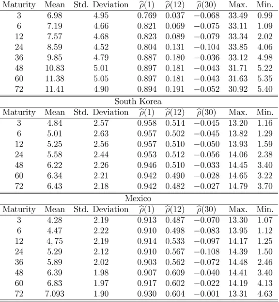
In this work it will be consider monthly zero-coupon bond yields. The maturities that will be used is …xed in 3, 6, 12, 24, 36,48, and 72 months, and they are obtained in the cubic spline process.
Brazil
Maturity Mean Std. Deviation b(1) b(12) b(30) Max. Min. 3 6:98 4:95 0:769 0:037 0:068 33:49 0:99 6 7:19 4:66 0:821 0:069 0:075 33:11 1:09 12 7:57 4:68 0:823 0:089 0:079 33:34 2:02 24 8:59 4:52 0:804 0:131 0:104 33:85 4:06 36 9:85 4:79 0:887 0:180 0:036 33:12 4:98 48 10:83 5:01 0:897 0:181 0:043 31:71 5:22 60 11:38 5:05 0:897 0:181 0:043 31:63 5:35 72 11:41 4:90 0:894 0:191 0:052 30:92 5:40
South Korea
Maturity Mean Std. Deviation b(1) b(12) b(30) Max. Min. 3 4:84 2:57 0:958 0:514 0:045 13:20 1:16 6 5:01 2:63 0:957 0:502 0:045 13:82 1:29 12 5:25 2:56 0:957 0:510 0:050 13:93 1:59 24 5:58 2:44 0:953 0:512 0:056 14:06 2:38 48 6:22 2:26 0:946 0:510 0:033 14:45 3:40 60 6:34 2:21 0:942 0:490 0:028 14:65 3:22 72 6:43 2:18 0:942 0:482 0:027 14:79 3:70
Mexico
Maturity Mean Std. Deviation b(1) b(12) b(30) Max. Min. 3 4:28 2:19 0:913 0:487 0:070 13:30 1:07 6 4:47 2:22 0:910 0:498 0:083 13:95 1:12 12 4;75 2:19 0:914 0:533 0:097 14:17 1:25 24 5:29 2:12 0:910 0:567 0:108 14:39 1:50 36 5:89 2:02 0:903 0:562 0:072 14:48 2:46 48 6:39 1:98 0:907 0:609 0:040 14:41 3:40 60 6:83 1:97 0:917 0:602 0:022 14:19 4:13 72 7:093 1:90 0:930 0:604 0:001 13:31 4:63
Maturity in months
Table 1: Summary Statistics for Yield Bond
the maturities, in the opposite of South Korea, and the average of …rst autocorrelation is0:87.
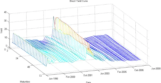
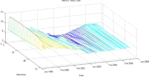
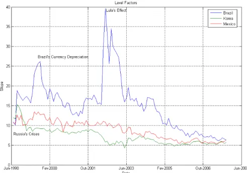
The …gure (3,4 and 5) show the government bond yield curves over countries and time. It is di¢cult to evaluate the bond yield curves in cross-country analysis, apparently the di¤erence are in the level of yield. The higher level certainly is in Brazil’s bond, which revels great increase near 2002. This crise was named Lula’s e¤ect. Lula was a principal candidate in the election, and his ideology was opposite of that was considered a good economy policy. It is important to note that South Korea and Mexico yield curves are better-behave in comparison with Brazil’s yield curve.
Figure 4: Yield Curve over Space and Time
4.1.3 Preliminary Analysis
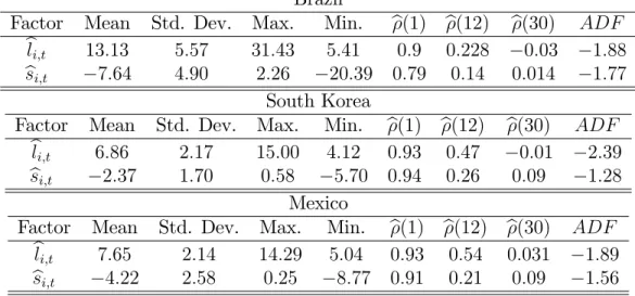
The multi-step estimation generated a lot of series and estimations that can be analyzed. Many of these estimates have important intuition about the desirable …nal results. In the …rst step of the model, it was extract the estimates level and slope,flit and sitg, t = 1; : : : ; T and i = 1; ::; N, following DL’s two step method. The …gure of these series can be viewed in (6) and (7).
The descriptive statistic for estimated factor indicates an autocorrelation the persistent dynamics. In general, the level factor correlograma indicates that its revel more persistent that slope factor. The Augmented Dickey-Fuller test did not reject the existence of unit root in both of factors in all countries. The existence of unit root is controversy in the nominal bond yields. The theory shows that the root is less that one, because, if it does not occurs, the nominal bond yield would eventually go to negative, that is not an acceptable. In DBY’s work, similar results are obtained.
Brazil
Factor Mean Std. Dev. Max. Min. b(1) b(12) b(30) ADF
b
li;t 13:13 5:57 31:43 5:41 0:9 0:228 0:03 1:88
b
si;t 7:64 4:90 2:26 20:39 0:79 0:14 0:014 1:77 South Korea
Factor Mean Std. Dev. Max. Min. b(1) b(12) b(30) ADF
bli;t 6:86 2:17 15:00 4:12 0:93 0:47 0:01 2:39
b
si;t 2:37 1:70 0:58 5:70 0:94 0:26 0:09 1:28 Mexico
Factor Mean Std. Dev. Max. Min. b(1) b(12) b(30) ADF
bli;t 7:65 2:14 14:29 5:04 0:93 0:54 0:031 1:89
b
si;t 4:22 2:58 0:25 8:77 0:91 0:21 0:09 1:56 ADF Denotes an argumented Dicky-Fuller test Statistic
Table 2: Descriptive Statistics for Estimated Factors
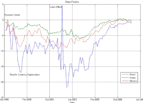
The graphics of the factors are plotted separately by factor. The graphic of both factors indicate that Brazil su¤er a big oscillation in 2002, when other did not have great variation in the period9.
The estimation follow DL described in the text
The estimation follow DL described in the text
Figure 7: Slope Factor using DL
An important insight arises when these …gures are analyzed. In the internal crises periods is important to note that both, level and slope factors are not connected across countries. Lula’s crisis in 2002 is the best example of this fact. During international crises, like Russia’s crises in 1998 it is possible to note that both, level and slope are connected. This characteristic infer that in the normal period, like after 2006 the curves are linked, and it explain the actual expectation in Brazil to obtain the investment grade from risk agencies, investiment grede already obtained for Mexico and korea. The curves show also that the level, that is linked with in‡ation, of yields are converging for stability and the same convergency is obtained for slope factor, that is linked with GDP.
The analysis of these curves can infer about the global factor results. The global factor are extracted take in account that existence of connections between the curves. DLY used the set of developed countries and the comparative analysis between these two set of countries it is possible to note that the oscilations in level and slope factor in developed markets is smoothest; the opposite is expected to occur in emerging markets, because of the internal oscillation in the curve.
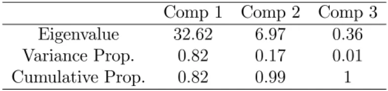
movements. Despite of the variability, it is possible to note that the dynamics of the factors run in the same directions. This evidence can be better described using the principal components framework. The PCA (principal components analysis) indicate the existence of global level and slope factor. The …rst principal component for level explains more than eighty percent of variation and the …rst principal component of slope explain more that ninety percent of variation.
Comp 1 Comp 2 Comp 3 Eigenvalue 32:62 6:97 0:36
Variance Prop. 0:82 0:17 0:01
Cumulative Prop. 0:82 0:99 1
Table 3: Principal Components Analysis for Estimated Level Factor
Comp 1 Comp 2 Comp 3 Eigenvalue 30:31 2:34 0:48
Variance Prop. 0:92 0:07 0:01
Cumulative Prop. 0:92 0:99 1
Table 4: Principal Components Analysis for Estimated Slope Factor
4.2
Results
The level and slope factors used are provided in the …rst step regression, using DL’s method. In the second step it was used the Kalman Filter to evaluate the likelihood function which the maximization is made by Marquart algorithm with convergence criteria of0:0001.
The Kalman …lter was initialized using the diagonal covariance matrix of state vector, and the initial parameters was choose using the V AR(1) processes of …rst
step using the level and slope principal components series in place of the latent global yield factors.
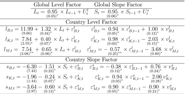
Global Level Factor Global Slope Factor
Lt= 0:95
(0:05) Lt 1+U
l
t St= 0:95
(0:06) St 1+U
s t
Country Level Factor
lB;t = 11:99
(9:60) + 1(0::34)32 Lt+"
l
B;t "lB;t = 0:94
(0:05) "
l
B;t 1+ 1:00 (0:12) v
l B;t
lK;t = 7:84
(2:55) + 0(0::07)40 Lt+"
l
K;t "lK;t= 0:98
(0:03) "
l
K;t 1 2:03 (0:15) v
l K;t
lM;t= 7:54
(3:08) + 0(0::06)65 Lt+"
l
M;t "lM;t = 0:57
(0:25) "
l
M;t 1 3:68 (0:80) v
l M;t Country Slope Factor
sB;t = 6:30
(7:43) (01::23)51 St+"
s
B;t "sB;t = 0:38
(0:12) "
s
B;t 1+ 0:76 (0:24) v
s B;t
sK;t = 1:96
(1:44) (00::07)24 St+"
s
K;t "sK;t= 0:94
(0:05) "
s
K;t 1 2:06 (0:28) v
s K;t
sM;t= 3:64
(2:97) (00::13)60 St+"
s
M;t "sM;t= 0:90
(0:05) "
s
M;t 1 0:90 (0:21) v
s M;t
Note-The numbers in the parentesis represents the standard Deviation , One asterisk Indicate that is signi…cant at 1 percent, two asterisk Indicate that is signi…cant at 5 percent
Table 5: Estimates of Global Yield Curve Models
Figure 9: Global Slope Factor vs. PCA of Slope
Some interesting conclusions can be made analyzing table of result and graphics. The level factor in‡uence Brazil’s level more than two other country, the in‡uence in the level factor is1:32 while in Korea and Mexico are 0:40and 0:65 respectively.
For instance, in some date of global level, the index can be near from 9:00, so in Brazil the in‡uence is 32% higher than global level, and in Korea and Mexico 40%
and 65% less than level yield curve. Another conclusion about the graphic of global
level curve is that there is a tendency to negative numbers that mean that the level of yield decreased during the period. Some similar characteristic can be found in DLY for global level curve. The slope curve in all cauntries su¤ers low in‡uence for global slope factor because the curve is around the zero and the result is very di¤erent of DLY. The answerer key to this question comes from the level of yield in these countries. The slope factor can be described as some sort run tendency of yield curve. In developed countries the level yield are lower than emerging countries and because of this the tendency for changes in the level in sort run or even the volatility tend to be higher than in emerging countries.
4.2.1 Variance Decomposition
The variance of speci…c country factor can be explained as a variation of global and idiosyncratic factors. It is important to evaluate this decomposition because this can explain the magnitude of variations of each factor, and infers the in‡uence of global movements in the country economy.
The formulation of country factor can be extracted from equation (12a and 12b) using a simple de…nition of variance, hence:
var(li;t) = li
2
var(Lt) +var("li;t)
var(si;t) = ( si)
2
var(St) +var("si;t)
In the Kalman …lter estimation, the extraction of the global and idiosyncratic factors may be correlated even if the global and idiosyncratic factors are not cor-related. The last speci…cation of factor’s variance obligate that these variables are orthogonal, and using the Kalman …lter’s estimations is not correct to decompose those variances. Hence, the orthogonalization will be obtained regressing the coun-tries factors on the global extracted factor and the results of these estimations will be used in the decomposition formulate.
li;t = cli+ l i L
Global t +"
l i;t
si;t = csi + s i S
Global t +"
s i;t
The resulta are:
Level Factors Volatility
Brazil South Korea Mexico Global Factor 44:69% 26:61% 7:29%
Idiosyncratic Factor 55:31% 73:39% 92:71%
Slope Factors Volatility
Brazil South Korea Mexico Global Factor 14:00% 0:03% 0:00
Idiosyncratic Factor 86:00% 99:97% 100:00%
Table 6: Variance Decomposition
5
Conclusion
The present work has extended the DLY studies about global yield curve that covered the developed countries. The proposal of this study is to extend the seminal work to emerging markets’ countries. The perception of emerging market su¤ers in‡uence of external factors or global factors, is the main argument of this work.
The seminal work of global yield curve extended the parsimonious yield curve proposed by NS and DL to a global environment. That work proposed the hierar-chical model in which country yield level and slope factor may depend on the global factors, as well as idiosyncratic factors. This work already uses a monthly data set of Brazil, South Korea and Mexico’s zero-coupon bond yield from June of 1998 to September of 2007 and using the McCulloch’s (1977) cubic spline to extract the unobserved maturities.
The results indicate, in concordance of DLY that level global factor have large in‡uence in the countries’ yield in special in Brazil’s yield curve because of the Brazil’s vulnerability of external crises, and the global level has a negative tendency that explain the decrease of emerging countries yield in recently years. The opposite result, now in discordance of DLY, about slope global factor can be found. The global slope factor can be interpreted as the sort run tendency of yield, and in developed countries the level of yield are lower than emerging countries and the tendency to increase their yield’s level are lower than developed countries, in order to highest level yield.
The results about the in‡uence of global factors variability in country variability obey the stylized facts. The in‡uence of global level factor variability in Brazils’ level factor is higher than other two, in order to Brazils’ vulnerability, and the global level factor vulnerability in‡uence the Mexico level yield less that other two, in order to Mexico is the US proxy. The results of global slope factor variability again respect the stylized facts, because of the level’s yield of emerging countries. The level’s yield in develop countries are lower than emerging countries, and because of this the variability is higher than emerging countries.
6
Bibliography
References
[1] Ang,A. and Piazzesi, M.(2003),"A No-Arbitrage Vector Autoregressin of Term Structure Dynamics with Macroeconomics and Latent Variables", Journal of Monetary Economics,50,745-787.
[2] Anderson, T. G. and Lund, J. (1997), "Stochastic Volatility and Mean Drift in the Short Term Interest Rate Di¤usion: Source of Steepness, Level, and Curvature in the Yield Curve",Working Paper 214, Departament of Finance, Kellog Scholl, Northwesterm University.
[3] Balduzzi, P.,Das, S.R.,Foresi,Sundaram, R. (1996),"A Simple Approach to Three-Factor A¢ne Term Structure Models", Journal of Fix Income, 6 , 43-53.
[4] Bliss, R. (1997a), "Movements in the Term Structure of Interest Rates", Eco-nomic Review, Federal Reserve Bank of Atlanta, 82 ,16-33.
[5] Bliss, R. (1997b),"Testing Term Structure Estimation Methods", Advanced in Finance and Options Research, 9 , 97-231.
[6] Brenna, M.J. and Xia, Y. (2006), "International Capital Makets and Foreign Exchange Risk", Review of Financial Studies, 19, 753-795.
[7] Campbell, J.Y., Lo, A.W. and Mackinley, A.C.,"The Econometrics of Financial Markets",Princeton University Press, Princeton, New Jersey.
[8] Cochrane, J. H.,"Asset Pricing", Princeton University Press, Princeton, New Jersey.
[9] Dai, Q. And Singleton, K. (2000), "Speci…cation Analysis of A¢ne Term Struc-ture Models", Journal of Finance, 55 , 1943-1978.
[10] Diebold, F.X. and Li, C. (2006), "Forecasting the Term Structure of Goverment Bond Yields", Journal of Econometrics, 130 , 337-364.
[12] Diebold, F.X., Rudebusch, G.D., and Aruoba, S.B.(2006), "Macroeconomics and Yield Curve: A Dynamic Latent Factor Approach", Journal of Econo-metrics, 131, 309-338.
[13] Fama, E. And Bliss, R. (1987),"The information in Long-Maturity Forward Rates", American Economic Review, 77, 680-692.
[14] Litterman R. and Scheinkman, J. (1991),"Common Factors A¤ecting Bond Re-turns", Journal of Fix Income, 1 , 49-53.
[15] McCulloch,J. H. (1971), "Measuring the Term Structure of Interest rates", Jour-nal of Bussines, 34, 19-31.
[16] McCulloch,J. H. (1975), "The Tax-adjusted Yield Curve", Journal of Finance, 30, 811-829.
[17] Nelsom, C.R. and Siegel, A.F. (1987),"Parsimonious Modeling of Yield Curves", Journal of Bussines, 60, 473-489.
[18] Sargent, T. and Sims, C.A.(1977),"Bussines Cycle Modeling Without Pretend-ing to Have too Much A Priori Economic Theory", in C. Sims (ed.), New Methods of Bussines Cycle Research. Minnepolis: Federal Reserve Bank of Minneapolis, 45-110.
[19] Solnik, B. (2004),"Intenational Investments"(4th Edition), New York: Addison Wesley.
[20] Stock, J. H. and Watson, M. W. (1989)," New Index of Coincidence and Leading conomic Indicators", NBER Macroeconomics Annual, 351-393.
APPENDIX A - CUBIC SPLINE
Spline
The discount function gives the present value of$1:00which is repaid in m years. Hence, the correspondent yield to maturity of investmenty(m);orspot interest rate, or zero coupon rates, must satisfy the following equation under continuous com-pounding:
d(m)e y(m) m = 1
d(m) =e y(m) m
The de…nition of discount function and spline method can be expressed using k
continuously di¤erentiable functions sj(m)to approximate the discount rates:
y(m) =a0+
k
X
j=1
ajsj(m) (22a)
or
d(m) = a0+
k
X
j=1
ajsj(m (22b)
Where sj(m) are known functions of maturities m, and a are the unknown co-e¢cients to be determined from the data. Since the discount rate must satisfy the constraint d(0) = 1, set a0 = 1 and sj(0) = 0 for j = 1; : : : k, and once the func-tional form ofs(m)is determined, the coe¢cients a can be easily estimated by linear regression.
McCulloch(1971) used the quadratic spline, which uses quadratic polynomial for
sj(m), and McCulloch(1977) used the cubic spline, which uses cubic polynomial. MacCulloch’s choice is based on fact that a polynomial function is easy to evaluate, di¤erentiate and integrate.
In Bliss(1996) was tested di¤erent methods to evaluate interpolations, and Bliss conclude that Unsmoothed Fama-Bliss(1987) is better than the others, but the dif-ference between it and cubic spline is small, because of this in this work it will be used McCulloch’s cubic spline for computational convenience, following Brennan and Xia (2003).
Consider these points:
(m0; Y0);(m1; Y1); : : :(mn 1; Yn 1);(mn; Yn): Using this points it is possible to …t cubic spline through the data.
Maturities
) , ( m 0 s 0
) ,
( m n s n
) , (m n−1 sn−1
) ,
( m 1 s 1
)
( m
s j
Figure 10: Interpolation of dicrete data
The splines are given by:
s1(m) = '1m3+ 1m2 + 1m+ 1 m0 m m1
s2(m) = '2m3+ 2m2 + 2m+ 2 m1 m m2
: :
sn(m) = 'nm3+ nm2+ nm+ n mn 1 x mn
The solution for4n coe¢cients is solved using simultaneous linear equations. The
question that arisen is the numbers of equations is the same of variables? There are needs to …nd4n equations for4n coe¢cients and it can be made di¤erentiating the
Having these coe¢cients, one can use equation (22a or 22b ) and …nd the para-meters'.