2016 | Lavras | Editora UFLA | www.editora.ufla.br | www.scielo.br/cagro
Spatial dependence and experimental precision in snap bean (
Phaseolus
vulgaris
L.) trials related to the number of plants and harvests
Dependência espacial e precisão experimental em ensaios com feijão-de-vagem
(Phaseolus vulgaris L.) relacionadas aos números de plantas e de colheitas
Alessandro Dal’Col Lúcio1*, Vilson Benz1, Lindolfo Storck1, Alberto Cargnelutti Filho1
1Universidade Federal de Santa Maria/UFSM, Departamento de Fitotecnia, Santa Maria, RS, Brasil *Corresponding author: [email protected]
Received in december 21, 2015 and approved in january 8, 2016
ABSTRACT
The productive variability in horticultural crops affects the planning and quality of the experiments, leading to wrong conclusions. The objectives of this study were to verify the spatial dependence of the fresh biomass of snap beans and to dimension the number of plants and harvests that are necessary to improve experimental accuracy in trials. The data of the fresh biomass of snap beans from uniformity trials carried out in a greenhouse and in the field with semivariograms were created with data transformed into indicators. Thus, they were combined on scenarios of plot size and harvest grouping, and they were adjusted to the spherical, exponential and Gaussian models. A response surface was also applied, with the variation coefficient as a dependent variable and the numbers of plants per plot and harvests as independent variables. The estimates of the semivariogram models parameters indicated a weak spatial dependence. The average of the fresh biomass of snap beans is distributed randomly in the trials, and it is not influenced by the number of plants per plot or by the number of grouped harvests. The best combinations between the number of plants per plot and harvest, for the smaller variation coefficients, are plots of 24 plants for plastic greenhouse and field, and 28 plants for plastic tunnel, in the autumn-winter, combined with the grouping of all harvests. In the spring-summer the number of plants per plot was 30 for plastic tunnel and field, also combined with
the grouping of all harvests.
Index terms: Geostatistic; spatial variability; multiple regression models; experiment planning; variation coefficient.
RESUMO
A variabilidade produtiva em cultivos olericolas afeta o planejamento e a qualidade de experimentos, levando a conclusões errôneas. Os objetivos foram verificar a dependência espacial da fitomassa fresca de vagens de feijão-de-vagem e dimensionar os números de plantas e de colheitas para melhor precisão experimental. Com os dados da fitomassa fresca de vagens de ensaios realizados em cultivo protegido e a campo com feijão-de-vagem foram ajustados semivariogramas com os dados transformados em indicadores. Foram combinados diferentes tamanhos de parcela e de agrupamentos de colheitas, sendo ajustados os modelos teóricos esférico, exponencial e gaussiano. Também foi ajustado um modelo de superfície de resposta tendo como variável dependente o coeficiente de variação e, como independentes, os números de plantas por parcela e de colheitas. As estimativas dos parâmetros dos modelos teóricos de semivariograma indicaram fraca dependência espacial. A média de fitomassa fresca de vagens possui distribuição aleatória nos ensaios, não sofrendo influência do número de plantas por parcela ou do número de colheitas agrupadas. As melhores combinações entre os números de plantas por parcela e de colheitas, para os menores coeficientes de variação e maior precisão experimental, são parcelas de 24 plantas, para os ensaios realizados em estufa plástica e a campo e 28 plantas para os ensaios em túnel plástico, no outono-inverno, combinados com o agrupamento de todas as colheitas. Na primavera-verão o número de plantas por parcela foi de 30 para os ensaios em túnel plástico e cultivo a campo, também combinados com o agrupamento de todas as colheitas.
Termos para indexação: Geoestatística; variabilidade espacial; modelos de regressão múltipla; planejamento de
experimentos; coeficiente de variação.
INTRODUCTION
Snap beans (Phaseolus vulgaris L.) are the most important Fabacea in the horticultural group. They are different from the common beans because they are harvested still in their immature stage, and they are used in human feeding in an industrialized manner and “in natura”
(Filgueira, 2008). Their growth is a good alternative for the off season period of other horticultural crops to diversify the production, both in protected environments and in the
field. This happens due to the use of staking structures and residual fertilization, serving also to break the cycle
In 2011 the production of vegetable crops in Brazil was 19.4 million ton and acreage of 537,215 ha with 17 principal vegetables (Associação Brasileira do Comércio de Sementes e Mudas-ABCSEM, 2011). The Southeast and South regions held three quarters of the production volume, while the Northeast and Midwest regions produced 25% of the total (Melo; Vilela, 2007).
So, the increase of the production and productivity
of horticultural crops, there was a generation of new technology, and that was also possible via application of experiments with consistent techniques. In those cases, the residual variability control generates improvements in accuracy, in the experimental quality, and in the reliability of inferences.
In horticultural in greenhouse crops, factors such as the position of the crop row in relation to the lateral doors, the presence or absence of fruits able to be harvested are variability causes that must be controlled during the execution of experiments. According to Lúcio et al. (2006), the injuries to which the plants are subjected during crop treatments and fruit harvesting, as well as the environmental variations, alter the plants individual production throughout the crops and, therefore, they become sources of variability as well.
Plots with no production are frequent, due to the absence of fruits that can be harvested or the fruits do not present appropriate characteristics for the harvest or commercialization. The occurrence of many plots with null values generates overdispersion in data. To reduce this overdispersion, Couto et al. (2009) suggest the use of plot size with more than one plant, combined with a grouping of harvests. In this sense, the application of geostatistic techniques to describe the spatial dependence on the experimental environments is useful to obtain a higher precision and reliability of the results.
Generally, according to Yamamoto and Landim (2013), through the geostatistic methodology it is possible to extract from an apparent random data the probabilistic structural characteristics of the regionalized phenomenon, that is, a correlation between the values located in a certain neighborhood and direction of sampling space. Fagioli,
Zimback and Landim (2012) reported that the geostatistic
assumes that the data are spatially related, and the closest points are more similar than the distant ones. Because of
that, we need to know the location in space of the variable
being studied in order to verify the existence and the spatial dependence level in a certain situation.
Many are the factors responsible for the occurrence of spatial dependence and it is not always possible to extrapolate the results obtained in an experimental
environment to others, since each one has specific characteristics (Yamamoto; Landim, 2013). However, respecting some limitations, the information can be useful, enabling the enhancement of the experimental techniques used.
The definitions of plot size and shape, number
of repetitions, sample size and experimental design are
influenced by the variability that exist in the experiment (Steel; Torrie; Dickey, 1997). This variability also interferes in the statistical analysis, inflating the experimental error,
leading the researcher to interpretations and conclusions which have low experimental accuracy and reliability in the results.
Authors such as Lopes et al. (1998), Lorentz et al. (2005), Lúcio et al. (2008), Carpes et al. (2008) and Couto et al. (2009) pointed out that there is a variability among
the crop rows and the multiple harvests. They also affirmed
that this variability alters the sampling intensity estimates, the size and form of the plot, the experimental design and the number of enough harvests to better discriminate between the treatments studied.
One of the alternatives to evaluate the variability in the experimental area is the use of uniformity tests, where the area is cultivated with and identical cultural practices, without applying treatments. After that, the area is divided in basic units, in which the variable observed in each basic units (BU) is measured separately, in a way that the values observed in the BU’s may be summed up
to simulate plots of different sizes and forms (Storck et
al., 2011). From the results generated in these trials, there is an investigation on the variability behavior among the plots and the harvests.
There are several papers defining the number of
plants per plot in experiments with horticulture of multiple harvests (Mello et al., 2004; Lorentz et al., 2005; Carpes et al., 2010; Lúcio et al., 2010; Santos et al., 2012). However,
there is a lack of papers that associate this size to the
number of harvests that should be done so that there is a smaller variability in the data and greater experimental accuracy in the conclusions. If the lower variability is associated with a lower number of harvests, it is possible to reduce the time necessary to evaluate the treatments. This way, it will not be necessary to wait until the end of the crop cycle, saving time, resources, and avoiding greater variation in the data observed.
MATERIAL AND METHODS
The data used was the fresh biomass of beans from snap beans (Phaseolus vulgaris L.) from the “macarrão” cultivar were used, obtained in uniformity trials carried out in the experimental area of the Federal University of Santa Maria, with coordinates 29º 43’ 23’’ S and 53º 43’ 15’’ W and altitude of 95 m. The climate of the region is
classified as Cfa humid subtropical, without dry season and with hot summers, according to the KÖPPEN classification (Moreno, 1961) and the soil classified as Paleudalf soil
(Empresa Brasileira de Pesquisa Agropecuária-Embrapa, 1999).
The trials were carried out in autumn-winter in three environments (plastic greenhouse, plastic tunnel and
field crops) and in spring-summer in two environments (plastic tunnel and field crop). The trial in the plastic
greenhouse was composed of six crop rows of 72 plants,
while in the plastic tunnels and in the crop fields there were
six rows of 84 plants, with spacing among the plants of 0.2 m and among the rows of 1m. The basic units (BU) were composed of two plants, totaling 36 BU’s in the plastic greenhouse and 42 BU’s in the plastic tunnel and
in the crop field. It was performes four harvests for each
environment in the trials during autumn-winter season and three crops during spring-summer season.
In all trials, the BUs were identified by the number
of crop row and were numbered according to their position inside the row. Several plot sizes with the data of the fresh biomass of the beans were elaborated summing up the adjacent BUs in the crop rows (1, 2, 3, 4, 6, 9, 12 and 18 BUs in the plastic greenhouse environment and 1, 2, 3, 6, 7, 14 and 21 BUs in plastic tunnel and
crop field) and two forms of harvest groupings. The first form of grouping was with the sum of consecutive
harvests, as follows: 1st, 1st + 2nd, 1st + 2nd + 3rd, and 1st+2nd+3rd+4th. The second form of grouping was with individual harvests, grouped 1st+2nd, grouped 3rd+4th and 1st+2nd+3rd+4th, in the autumn-winter season and individual harvests, grouped 1st+2nd, grouped 2nd+3rd and 1st+2nd+3rd in the spring-summer season. For each
plot and harvest carried out, a variation coefficient (%)
was estimated at the crop row.
For the geostatistic analysis, the data from the fresh biomass of beans of the plot sizes and number of harvests were georeferenced in UTM coordinates in function of the distances (in meters), generating a point grid inside each crop row. The greatest number of plot for each trial was the one in which there were at least 30 points for the analysis, as Landim (2006) recommends. The original data of the
fresh biomass of beans were transformed into indicators using the general average as a cutoff level, according to the criterion proposed by Yamamoto and Landim (2013),
where: vt = 1 if vj ≤ vc and vt = 0 if vj > vc, in which
vt = transformed value, vc = cutoff level (average); vj = variable observed value.
A semivariogram was elaborated according to the description by Vieira et al. (1983) by the equation:
N(h) 2
i i h
i 1
1
* (h) [ (X ) Z(X )]
2N(h)
γ +
=
=
∑
Σ − , w h e r eN(h) is the number of pairs of values Z(xi) and Z(xi+h) separated by the hr distance. The chart of versus the values corresponding to h is the semivariogram where the spherical, exponential and Gaussian theoretical models were adjusted. In the adjustment of the theoretical models to the experimental semivariograms, the nugget effect (Co), the contribution (C1), the sill (Co + C1) and the range (R) were calculated.
For the analysis of the spatial dependence index (SDI), the ratio SDI= C1/(C1+Co)*100 was used, as well as the intervals descript in Souza et al. (2008) who
considers: weak (SDI < 25%), moderate (25% ≤ SDI < 75%) and strong (SDI ≥ 75%) spatial dependence. In case the SDI ≥ 25%, the elaboration of the maps with classes of
probability of the plots to produce above the average were
carried out through the indicative kriging and the studies
of the variability behavior that was carried out within each one of the probability classes in the uniformity trial.
In cases where SDI < 25%, the variability behavior study
was carried out in the whole trial.
In order to scale the number of plants and harvests necessary to reduce the variability of the experiments, a second-order polynomial regression was used, described by Neter and Wasserman (1996) as: Y=β0+β1X1+β11X12+
2
2X2 22X2 12X X1 2 i
β +β +β +ε , in which Y= is the
variation coefficient between the plots within the crop row,
X1= plot size and X2= number of harvests. The model was rewritten in matrix notation Yˆ =βˆ0+X 'aˆ+X ' AXˆ ,
in which: 1
2 X X X =
contains the values of the pair whose
answer’s estimate is desired; 1
2 ˆ ˆa ˆ β β =
formed by the
linear coefficients of the equation; and,
12 11 21 22 ˆ ˆ 2 ˆ A ˆ ˆ 2 β β β β =
surface a response function of the critical point was estimated by X* 1 ˆ ˆA a1
2
− −
= . The maximum or minimum
nature of the critical point was identified by the signal of the eigenvalues associated to the matrix Â, that is, you find
the values λ λ λ= 1 2 so that the determinant of (Aˆ−λI) equals zero (I= identity matrix).
The regression equations were estimated with the help of the Genes application (Cruz, 2013) and the geostatistic procedures were carried out with the computing program ArcGis 10.1 (Enviromental Systems Research Institute-Esri, 2012).
RESULTS AND DISCUSSION
The spatial dependence indexes (SDI) obtained in the scenarios of plot size and harvest group were generally low (Tables 1, 2 and 3). That way, the variations in fresh mass of the fruits do not have any structure depending on the distance between the sampling points. In this condition, it is not
recommended the use of indicative kriging for the definition of probability classes and the area of the trials
environment were studied integrally.
Almost all the adjusted semivariogram models
presented weak or moderate spatial dependence (SDI<
75%). These results indicate that the average of fresh biomass of beans is distributed randomly within the experimental area grown with snap beans, for any plot size and form of grouping. These results agree with those obtained by Benz, Lúcio and Lopes (2015), who found the random distribution of the zucchini production under different plot sizes and with the grouping of the
three first harvests. However, in a greenhouse crop of
tomatoes and in crops of melon in two commercial production areas with different soils, hybrid and cultural treatment (Miranda et al., 2005), the variability and spatial dependence seen was from moderate to strong in all the production components and crop systems.
In most adjusted models, the value of the variogram function at the origin, called the nugget effect, was distant from zero, and several models presented pure nugget effect (Tables 1, 2 and 3). What is more evident differences were spatial dependence values in
experiments carried out in the field and in protected
environments. During the autumn-winter season, the trial in plastic greenhouse presented 33.3% of models
with spatial dependence classified as moderate or strong, while the trials in plastic tunnel and in the field were 25%,
94.44%, respectively. In the spring-summer season, the trial in plastic tunnel presented 25.93% of the models with
moderate or strong SDI while in the field it was 85.88%. The SDI values were higher in the field, mostly, which
also did not present any combination with pure nugget effect in both season periods. In the trial at a plastic greenhouse, the lowest SDI or the pure nugget effect were observed with the use of four classes of grouped harvests, regardless of the plot size and the semivariogram model (Table 1).
In the theoretical models of semivariogram, we saw that, generally, the higher the nugget effect, the smaller the contribution (difference between the baseline and the nugget effect), the higher the quadratic average error and the smaller the spatial dependence found (Tables 1, 2 and 3). The similar RMSE values was also seen between the semivariogram models used (Tables 1, 2 and 3). This situation shows little difference among the models, being RMSE predominantly a
bit smaller in the first harvest in any plot size. In the
situations where there was a strong spatial dependence with the adjusted semivariogram theoretical model, this did not represent variability (Tables 1, 2 and 3).
In these cases, the lack of structure was visible in the
semivariogram, because the appropriate would be an increase in the semivariance with the distance until reaching the range, and what happened was the random
fluctuation of the semivariance. According to Landim
(2006), in a regionalized variable, the value of each point is related, somehow, to values obtained from points located at a certain distance, being reasonable
to infer that the influence is higher when the distance
between the points is smaller.
The fresh biomass of snap beans presents
variability influenced mainly by the weather conditions,
by the type of handling used and harvest time. According to Andriolo (2002), the field crops are subject to environmental variations because of the smaller control
of the temperature, humidity and wind inflating thus
Table 1: Geostatistic analysis for the snap bean trial in plastic greenhouse in the autumn-winter season.
NGH* Model Co C1 R RMSE SDI NC Model Co C1 R RMSE SDI
1 BU per Plot 2 BU per Plot
1
ESF 0.184 0.054 2.40 0.4712 22.80
1
ESF 0.160 0.090 2.60 0.4761 36.16 EXP 0.157 0.081 1.78 0.4739 34.17 EXP 0.034 0.215 1.63 0.4893 86.25
GAU 0.194 0.044 2.07 0.4713 18.66 GAU 0.178 0.072 2.23 0.4783 28.87
2
ESF 0.227 0.022 2.47 0.4939 8.85
2
ESF 0.145 0.112 3.00 0.4491 43.47 EXP 0.214 0.036 1.80 0.4942 14.25 EXP 0.046 0.212 2.27 0.4529 82.26
GAU 0.231 0.018 2.10 0.4940 7.22 GAU 0.170 0.087 2.70 0.4512 33.98
3
ESF 0.235 0.016 2.31 0.4996 6.42
3
ESF 0.222 0.029 2.72 0.4940 11.41
EXP 0.237 0.014 2.05 0.4992 5.69 EXP 0.185 0.065 1.50 0.5140 25.87
GAU 0.239 0.012 2.13 0.4991 4.75 GAU 0.229 0.021 2.25 0.4839 8.31
4
ESF 0.250 0.000 4.39 0.5125 0.13
4
ESF 0.245 0.000 15.00 0.5133 0.00 EXP 0.250 0.000 15.00 0.5125 0.00 EXP 0.245 0.000 15.00 0.5133 0.00
GAU 0.250 0.000 3.69 0.5125 0.14 GAU 0.245 0.000 15.00 0.5133 0.00
3 BU per Plot 4 BU per Plot
1
ESF 0.109 0.149 2.55 0.4583 57.72
1
ESF 0.107 0.147 2.65 0.4525 57.83 EXP 0.000 0.258 2.00 0.4600 100.00 EXP 0.003 0.251 2.00 0.4404 98.93
GAU 0.144 0.114 2.30 0.4585 44.33 GAU 0.136 0.117 2.22 0.4402 46.32
2
ESF 0.234 0.037 15.00 0.4995 13.66
2
ESF 0.215 0.041 2.75 0.5218 16.06
EXP 0.229 0.040 15.00 0.4974 14.98 EXP 0.216 0.040 2.36 0.5054 15.55
GAU 0.241 0.036 15.00 0.5018 13.03 GAU 0.231 0.025 2.65 0.5238 9.72
3
ESF 0.162 0.091 2.27 0.4918 36.05
3
ESF 0.211 0.044 2.65 0.5231 17.33 EXP 0.129 0.125 2.00 0.4938 49.14 EXP 0.201 0.054 2.00 0.5064 21.21
GAU 0.185 0.069 2.03 0.4924 26.99 GAU 0.225 0.030 2.33 0.5056 11.81
4
ESF 0.253 0.000 15.00 0.5337 0.00
4
ESF 0.207 0.045 2.22 0.5240 17.73 EXP 0.253 0.000 15.00 0.5337 0.00 EXP 0.249 0.003 2.00 0.5297 1.11
GAU 0.253 0.000 15.00 0.5337 0.00 GAU 0.227 0.025 2.00 0.5261 10.02 6 BU per Plot
1
ESF 0.116 0.147 3.23 0.4766 55.90
EXP 0.000 0.263 2.28 0.4761 100.00
GAU 0.136 0.127 2.55 0.4764 48.39
2
ESF 0.237 0.032 11.40 0.5122 11.82 EXP 0.233 0.037 14.00 0.5124 13.82
GAU 0.244 0.029 11.58 0.5122 10.61
3
ESF 0.257 0.000 14.00 0.5443 0.00 EXP 0.257 0.000 14.00 0.5443 0.00
GAU 0.257 0.000 14.00 0.5443 0.00
4
ESF 0.256 0.000 14.00 0.5404 0.00 EXP 0.256 0.000 14.00 0.5404 0.00
GAU 0.256 0.000 14.00 0.5404 0.00
Table 2: Geostatistic analysis for snap bean trial in plastic tunnel and in crop field, in the autumn-winter season.
Trial in plastic tunnel Field trial
NGH* Model Co C1 R RMSE SDI NC Model Co C1 R RMSE SDI
1 BU per Plot 1 BU per Plot
1
ESF 0.178 0.071 1.25 0.4988 28.63 1
ESF 0.211 0.064 11.55 0.4810 23.22 EXP 0.074 0.176 0.77 0.4912 70.30 EXP 0.199 0.079 12.88 0.4772 28.38
GAU 0.184 0.066 0.95 0.4916 26.28 GAU 0.221 0.054 9.99 0.4846 19.55
2
ESF 0.242 0.015 12.42 0.5173 5.84 2
ESF 0.205 0.087 13.93 0.4651 29.86
EXP 0.241 0.017 17.00 0.5170 6.73 EXP 0.193 0.103 17.00 0.4635 34.81
GAU 0.245 0.014 11.62 0.5178 5.26 GAU 0.217 0.077 12.34 0.4676 26.20
3
ESF 0.252 0.000 17.00 0.5151 0.00
3
ESF 0.152 0.214 17.00 0.4170 58.43 EXP 0.252 0.000 17.00 0.5151 0.00 EXP 0.129 0.214 17.00 0.4221 62.42
GAU 0.252 0.000 17.00 0.5151 0.00 GAU 0.176 0.184 13.43 0.4147 51.15
4
ESF 0.252 0.000 17.00 0.5232 0.00
4
ESF 0.174 0.165 17.00 0.4376 48.67 EXP 0.252 0.000 17.00 0.5232 0.00 EXP 0.156 0.168 17.00 0.4428 51.98
GAU 0.252 0.000 17.00 0.5232 0.00 GAU 0.194 0.147 14.01 0.4338 43.07
2 BU per Plot 2 BU per Plot
1
ESF 0.246 0.016 16.00 0.5064 6.25 1
ESF 0.206 0.089 14.10 0.5060 30.27 EXP 0.246 0.015 16.00 0.5070 5.63 EXP 0.195 0.100 16.00 0.5090 33.80
GAU 0.248 0.018 16.00 0.5055 6.88 GAU 0.217 0.083 12.64 0.5028 27.69
2
ESF 0.237 0.026 16.00 0.5136 9.93
2
ESF 0.183 0.144 16.00 0.4523 44.06 EXP 0.234 0.026 16.00 0.5129 10.10 EXP 0.163 0.153 16.00 0.4533 48.41
GAU 0.240 0.027 16.00 0.5144 10.25 GAU 0.203 0.136 14.75 0.4518 40.13
3
ESF 0.247 0.008 16.00 0.5143 3.07 3
ESF 0.135 0.235 16.00 0.3986 63.49
EXP 0.248 0.005 16.00 0.5144 2.10 EXP 0.107 0.242 16.00 0.3943 69.37
GAU 0.248 0.010 16.00 0.5141 3.89 GAU 0.168 0.242 16.00 0.4077 58.96
4
ESF 0.251 0.000 16.00 0.5281 0.00
4
ESF 0.177 0.155 16.00 0.4417 46.76 EXP 0.251 0.000 16.00 0.5281 0.00 EXP 0.156 0.164 16.00 0.4404 51.31
GAU 0.251 0.000 16.00 0.5281 0.00 GAU 0.200 0.157 16.00 0.4445 43.96
3 BU per Plot 3 BU per Plot
1
ESF 0.255 0.000 16.00 0.5339 0.00 1
ESF 0.180 0.102 7.53 0.4891 36.24 EXP 0.255 0.000 16.00 0.5339 0.00 EXP 0.143 0.140 6.95 0.4884 49.41
GAU 0.255 0.000 16.00 0.5339 0.00 GAU 0.199 0.083 6.79 0.4903 29.48
2
ESF 0.155 0.112 3.77 0.4799 42.02
2
ESF 0.117 0.260 14.55 0.3977 68.90 EXP 0.091 0.176 3.17 0.4818 65.85 EXP 0.085 0.285 16.00 0.4006 77.07
GAU 0.176 0.091 3.25 0.4784 34.17 GAU 0.151 0.229 12.22 0.3984 60.17
3
ESF 0.147 0.115 2.79 0.4830 44.07
3
ESF 0.115 0.272 16.00 0.3796 70.37 EXP 0.017 0.246 2.10 0.4827 93.53 EXP 0.080 0.284 16.00 0.3743 77.96
GAU 0.154 0.108 2.24 0.4814 41.17 GAU 0.154 0.279 16.00 0.3933 64.34
4
ESF 0.211 0.041 2.10 0.5204 16.31
4
ESF 0.115 0.272 16.00 0.3796 70.37 EXP 0.244 0.008 2.10 0.5215 3.03 EXP 0.080 0.284 16.00 0.3743 77.96 GAU 0.233 0.019 2.10 0.5208 7.53 GAU 0.154 0.279 16.00 0.3933 64.34
Table 3: Geostatistic analysis for snap bean trial in plastic tunnel and in crop field, in the spring-summer season.
Trial in plastic tunnel Field trial
NGH* Model Co C1 R RMSE SDI NC Model Co C1 R RMSE SDI
1 BU per Plot 1 BU per Plot
1
ESF 0.194 0.060 2.33 0.4846 23.63
1
ESF 0.162 0.097 3.17 0.4438 37.60 EXP 0.169 0.086 2.09 0.4879 33.66 EXP 0.143 0.119 3.62 0.4481 45.43
GAU 0.200 0.054 1.90 0.4841 21.14 GAU 0.178 0.081 2.78 0.4420 31.18
2
ESF 0.248 0.008 17.00 0.5295 3.29
2
ESF 0.086 0.170 1.79 0.4353 66.27
EXP 0.247 0.008 17.00 0.5295 3.30 EXP 0.023 0.235 1.67 0.4551 91.24
GAU 0.249 0.009 17.00 0.5295 3.38 GAU 0.117 0.139 1.59 0.4357 54.25
3
ESF 0.250 0.000 17.00 0.5314 0.00
3
ESF 0.233 0.020 3.49 0.5104 8.01 EXP 0.250 0.000 17.00 0.5314 0.00 EXP 0.232 0.021 3.08 0.5117 8.48
GAU 0.250 0.000 17.00 0.5314 0.00 GAU 0.236 0.018 2.97 0.5096 6.90
2 BU per Plot 2 BU per Plot
1
ESF 0.116 0.147 3.77 0.4258 55.88
1
ESF 0.000 0.258 1.96 0.3761 100.00 EXP 0.007 0.256 2.84 0.4276 97.27 EXP 0.000 0.264 2.59 0.3935 100.00
GAU 0.145 0.119 3.30 0.4301 45.14 GAU 0.000 0.259 1.58 0.3782 99.90
2
ESF 0.238 0.015 1.58 0.5705 5.93
2
ESF 0.000 0.260 1.84 0.3564 100.00 EXP 0.253 0.000 16.00 0.5266 0.00 EXP 0.000 0.262 2.03 0.3858 100.00
GAU 0.253 0.000 16.00 0.5266 0.00 GAU 0.000 0.262 1.58 0.3582 99.90
3
ESF 0.251 0.000 16.00 0.5296 0.00
3
ESF 0.151 0.111 3.11 0.4687 42.49 EXP 0.251 0.000 16.00 0.5296 0.00 EXP 0.044 0.217 2.14 0.4776 83.12
GAU 0.251 0.000 16.00 0.5296 0.00 GAU 0.174 0.089 2.74 0.4705 33.74
3 BU per Plot 3 BU per Plot
1
ESF 0.121 0.143 3.30 0.4367 54.25
1
ESF 0.114 0.148 2.46 0.4588 56.59 EXP 0.012 0.252 2.60 0.4377 95.55 EXP 0.050 0.214 2.40 0.4687 81.00
GAU 0.150 0.114 2.93 0.4360 43.01 GAU 0.162 0.101 2.48 0.4621 38.46
2
ESF 0.251 0.000 16.00 0.5298 0.00
2
ESF 0.140 0.122 3.02 0.4501 46.65 EXP 0.251 0.000 16.00 0.5298 0.00 EXP 0.059 0.205 2.66 0.4510 77.65
GAU 0.251 0.000 16.00 0.5298 0.00 GAU 0.149 0.113 2.44 0.4361 43.10
3
ESF 0.251 0.000 16.00 0.5306 0.00
3
ESF 0.082 0.177 2.10 0.4721 68.31 EXP 0.251 0.000 16.00 0.5306 0.00 EXP 0.063 0.197 2.10 0.4845 75.71
GAU 0.251 0.000 16.00 0.5306 0.00 GAU 0.155 0.105 2.10 0.4791 40.36
*NGH= number of grouped harvests; BU= basic units; Co= nugget effect; C1= contribution; R= range; RMSE= root mean square error; SDI= spatial dependence index; theoretical models of spherical semivariograms (ESF), exponential (EXP) and Gaussian (GAU).
Another factor that may have contributed for the absence of dependent structuring of the distance between the measurement points in the average variations of fresh biomass of snap beans may have originated in the structuring of the uniformity tests. For the scenarios of plot sizes, neighboring plants were grouped inside the crop row, which generated greater uniformity in the production values by the combination of plants in a similar
region. This methodology has been adopted by several authors (Lúcio et al., 2008; Carpes et al., 2010; Santos et al., 2014; Benz et al., 2015) due to the variability among the crop rows.
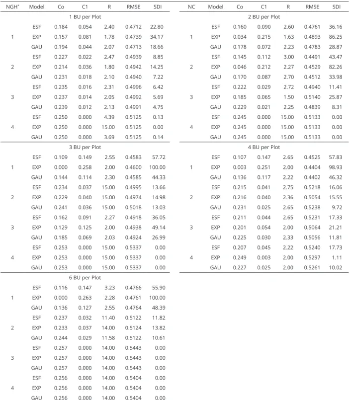
The polynomial equations adjusted were very similar to the two forms of harvest groupings. Among the three environments used, it was seen that the trial carried
18 15 12 9 6 3
Plot size
1 2
3
Harvestin g groups
0 10 20 30 40 50 60 70 80 90
VC
(
%)
Adjusted equation (a) X1 X2 R²
VC% = 115.785 - 8.906 X1 + 0.286 2
1
X - 34.697 X2 + 4.346 2 2
X + 0.562 X1X2 12.42 3.18 0.89
18 15 12 9 6 3
Plot size
1 2
3
Harvestin g groups
0 10 20 30 40 50 60 70 80
VC
(
%)
Adjusted equation (b) X1 X2 R²
VC% = 87.666 - 7.381 X1 + 0.259 2
1
X - 19.105 X2 + 2.132 2 2
X + 0.271 X1X2 12.30 3.69 0.90
Figure 1: Response surface of the variation coefficient (%) for fresh biomass of snap bean in function of the plot
sizes (X1) and harvest groups (X2), determination coefficient (R2) and critical point, in trial with snap beans in plastic
greenhouse during autumn-winter season for the first (a) and second (b) forms of harvest grouping. those in greenhouse and in plastic tunnel (Figures 1, 2,
3, 4 and 5).
It was possible to estimate the critical points of the
minimum variation coefficient (VC) in all cases studied
because the estimates of the eigenvalues of matrix were positive. In the autumn-winter season, the plot size with the minimum VC was 24 plants (X1 =12 UB) for the trials
carried out in a plastic greenhouse and in the field, and
28 plants (X1 = 14 UB) for those carried out in plastic
tunnel. For the spring-summer season, the plot size with minimum VC was 30 plants (X1 = 15 UB) for the trials in
plastic tunnel and in the field. In all uniformity trials, the
best harvest grouping was the use of the total produced, X2 near the maximum (Figures 1, 2, 3, 4 and 5).
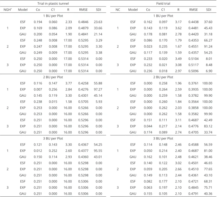
In experiments with snap beans, Santos et al. (2012)
verified that the estimates of the variation coefficients for
21 18 15 12 9 6 3
Plot size
1 2
3
Harvestin g group
s 0
5 10 15 20 25 30 35 40 45
VC
(
%)
Adjusted equation (a) X1 X2 R²
VC% = 52.753 - 4.134 X1 + 0.128 2 1
X - 11.745 X2 + 1.471 2 2
X + 0.092 X1X2 14.84 3.52 0.86
21 18 15 12 9 6 3
Plot size
1 2
3
Harvestin g group
s
0 10 20 30 40 50 60
VC
(
%)
Adjusted equation (b) X1 X2 R²
VC% = 64.638 - 5.001 X1 + 0.151 2
1
X - 14.106 X2 + 1.448 2 2
X + 0.164 X1X2 14.34 4.05 0.92
Figure 2: Response surface of the variation coefficient (%) for fresh biomass of snap bean in function of the plot
sizes (X1) and harvest groups (X2), determination coefficient (R2) and critical point, in trial with snap beans in plastic
tunnel during autumn-winter season for the first (a) and second (b) forms of harvest grouping. obtained with the harvest groupings. The same authors
concluded that the production analysis of beans per harvest, instead of total production, reduces the accuracy of the experiments with snap beans. Also, Haesbaert et al. (2011) observed that the production grouping of all harvests enables the use of smaller sample sizes than in the individual harvests or the ones grouped two by two,
because it enables a reduction of variation coefficient
values in most of the crop rows.
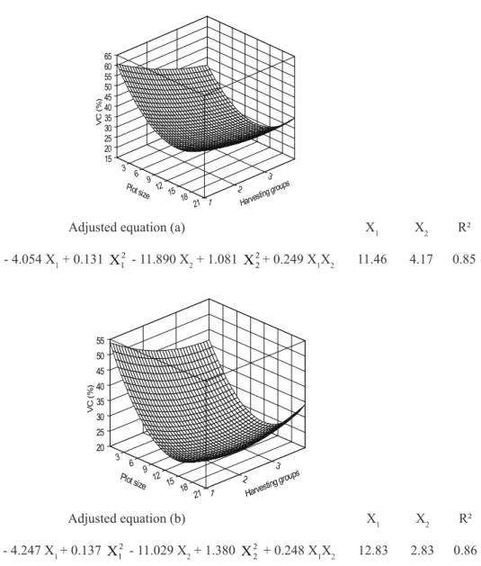
An experimental area with random variability (no spatial dependence) can be used for conduct experiments that used statistical analysis models, which assume the random distribution of errors. However, when variability is spatially correlated, the geostatistic techniques are useful for reducing the standard error of the means of treatments, to improve the discrimination in the treatments and to increase statistic test power (Duarte;
21 18 15 12 9 6 3
Plot size
1 2
3
Harvestin g group
s 15
20 25 30 35 40 45 50 55 60 65
VC
(
%)
Adjusted equation (a) X1 X2 R²
VC% = 71.476 - 4.054 X1 + 0.131 2
1
X - 11.890 X2 + 1.081 2 2
X + 0.249 X1X2 11.46 4.17 0.85
21 18 15 12 9 6 3
Plot size
1 2
3
Harvestin g groups
20 25 30 35 40 45 50 55
VC
(
%)
Adjusted equation (b) X1 X2 R²
VC% = 63.602 - 4.247 X1 + 0.137 2 1
X - 11.029 X2 + 1.380 2 2
X + 0.248 X1X2 12.83 2.83 0.86
Figure 3: Response surface of the variation coefficient (%) for fresh biomass of snap bean in function of the plot
sizes (X1) and harvest groups (X2), determination coefficient (R2) and critical point, in trial with snap beans in the
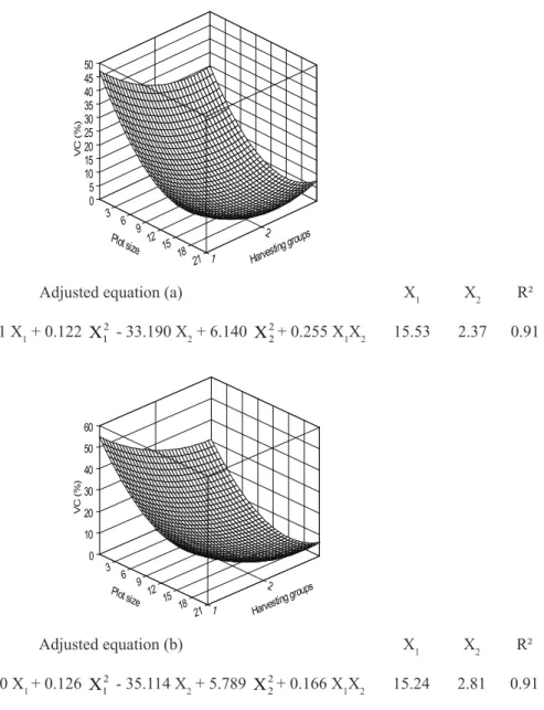
21 18 15 12 9 6 3
Plot size
1 2
Harvestin g group
s
0 5 10 15 20 25 30 35 40 45 50
VC
(
%)
Adjusted equation (a) X1 X2 R²
VC% = 74.229 - 4.411 X1 + 0.122 2
1
X - 33.190 X2 + 6.140 2 2
X + 0.255 X1X2 15.53 2.37 0.91
21 18 15 12 9 6 3
Plot size
1
2
Harvestin g groups 0
10 20 30 40 50 60
VC
(
%)
Adjusted equation (b) X1 X2 R²
VC% = 84.150 - 4.330 X1 + 0.126 2 1
X - 35.114 X2 + 5.789 2 2
X + 0.166 X1X2 15.24 2.81 0.91
Figure 4: Response surface of the variation coefficient (%) for fresh biomass of snap beans in function of the plot
sizes (X1) and harvest groups (X2), determination coefficient (R2) and critical point, in trial with snap beans in plastic
21 18 15 12 9 6 3
Plot size
1
2
Harvestin g group
s
0 10 20 30 40 50 60 70 80
VC
(
%)
Adjusted equation (a) X1 X2 R²
VC% = 117.004 - 5.100 X1 + 0.118 2 1
X - 54.075 X2 + 8.782 2 2
X + 0.575 X1X2 15.29 2.57 0.94
21 18 15 12 9 6 3
Plot size
1
2
Harvestin g group
s
0 10 20 30 40 50 60 70
VC
(
%)
Adjusted equation (b) X1 X2 R²
VC% = 94.641 - 4.319 X1+ 0.107 2
1
X - 39.552 X2 + 6.324 2 2
X + 0.403 X1X2 15.13 2.64 0.93
Figure 5: Response surface of the variation coefficient (%) for fresh biomass of snap beans in function of the plot
sizes (X1) and harvest groups (X2), determination coefficients (R2) and critical point, in trial with snap bean in the
field during spring-summer season for the first (a) and second (b) forms of harvest grouping.
The variation coefficient (VC) reduces with the
increase in the number of harvests grouped among the plots in the crop rows for the different plot sizes (Figures 1, 2, 3, 4 and 5). However, depending on the level of accuracy required, it is possible to reduce the plot size, increasing their number in the rows. In this case, the VC values obtained are increasingly higher, harming the accuracy of the production estimates.
CONCLUSIONS
The estimates of the parameters for the spherical, exponential and Gaussian semivariogram theoretical
models indicated a weak spatial dependence. The means
of the fresh biomass of snap bean is distributed randomly
in the environments, and it is not influenced by the plot
The smallest variation coefficients are observed
in plots of 24 plants for the trials carried out in plastic
greenhouse and in the field, and 28 plants for the trials in
plastic tunnel, in the autumn-winter season, combined with the grouping of all harvests. In the spring-summer season, the plot size is 30 plants for trials in plastic tunnel and in
the field, also combined with the grouping of all harvests.
ACKNOWLEDGEMENTS
We would like to thank the National Council for Scientific and Technological Development (CNPq/Brazil)
for the concession of research grant resources.
REFERENCES
ANDRIOLO, J. L. Olericultura geral: princípios e técnicas. Santa
Maria: UFSM, 2002. 158p.
ANDRIOTTI, J. L. S. Notas de Geoestatística. Estudos tecnológicos - Acta Geologica Leopoldensia,
25(55):3-14, 2002.
ASSOCIAÇÃO BRASILEIRA DO COMÉRCIO DE SEMENTES E MUDAS – ABCSEM. Projeto para levantamento dos dados socioeconômicos da cadeia produtiva de hortaliças no Brasil2010/2011. Campinas: ABCSEM, 2011. Available in:
<http:// www.abcsem.com.br/docs/direitos_resevados. pdf>. Access in: December 18, 2015.
BENZ, V.; LÚCIO, A. D.; LOPES, S. J. The spatial and temporal
independence of Italian Zucchini production. Acta Scientiarum, 37(2):257-263, 2015.
CARPES, R. H. et al. Ausência de frutos colhidos e suas interferências na variabilidade da fitomassa de frutos de
abobrinha italiana cultivada em diferentes sistemas de
irrigação. Revista Ceres,55(6):590-595, 2008.
CARPES, R. H. et al. Variabilidade produtiva e agrupamentos
de colheitas de abobrinha italiana cultivada em ambiente protegido. Ciência Rural, 40(2):294-301, 2010.
COUTO, M. R. M. et al. Transformação de dados em experimentos com abobrinha italiana em ambiente
protegido. Ciência Rural, 39(6):1701-1707, 2009.
CRUZ, C. D. Genes – a software package for analysis in experimental statistics and quantitative genetics. Acta Scientiarum – Agronomy, 35(3):271-276, 2013.
DUARTE, J. B.; VENCOVSKY, R. Spatial statistical analysis
and selection of genotypes in plant breeding. Pesquisa Agropecuária Brasileira, 40(2):107-114, 2005.
EMPRESA BRASILEIRA DE PESQUISA AGROPECUÁRIA - EMBRAPA. Centro Nacional de Pesquisa de Solos. Sistema Brasileiro de Classificação de Solos. Brasília, 1999. 412p.
ENVIRONMENTAL SYSTEMS RESEARCH INSTITUTE-ESRI. ArcGIS Spatial Analysis: Release 10.1. Redlands, CA: ESRI, 2012.
FAGIOLI, A. S.; ZIMBACK, C. R. L.; LANDIM, P. M. B. Classificação
de imagens em áreas cultivadas com citros por técnicas de sensoriamento remoto e geoestatística. Revista Energia na Agricultura, 27(3):01-15, 2012.
FILGUEIRA, F. A. R. Agrotecnologia moderna na produção e comercialização de hortaliças. Novo manual de olericultura, 3.ed.Viçosa: Editora UFV, 2008. 421p.
HAESBAERT, F. M. et al. Tamanho de amostra para experimentos com feijão-de-vagem em diferentes ambientes. Ciência Rural, 41(1):38-44, 2011.
LANDIM, P. M. B. Sobre geoestatística e mapas. Terra e Didática, 2(1):19-33, 2006.
LOPES, S. J. et al. Técnicas experimentais para tomateiro tipo
salada sob estufas plásticas. Ciência Rural, 28(2):193-197,
1998.
LORENTZ, L. H. et al. Variabilidade da produção de frutos de pimentão em estufa plástica. Ciência Rural,
35(2):316-323, 2005.
LÚCIO, A. D. et al. Variação temporal da produção de pimentão influenciada pela posição e características morfológicas das
plantas em ambiente protegido. Horticultura Brasileira,
24(1):31-35, 2006.
__________________. Variância e média da massa de frutos de abobrinha-italiana em múltiplas colheitas. Horticultura Brasileira, 26(3):335-341, 2008.
__________________. Agrupamento de colheitas de tomate e
estimativas do tamanho de parcela em cultivo protegido.
Horticultura Brasileira, 28(2):190-196, 2010.
MELLO, R. M. et al. Size and form of plots for the culture of the italian pumpkin in plastic greenhouse. Scientia Agricola,
61(4):457- 461, 2004.
MELO, P. C. T.; VILELA, N. J. Importância da cadeia produtiva brasileira de hortaliças. In: 13ª Reunião ordinária da
MIRANDA, N. O. et al. Variabilidade espacial da produtividade
do meloeiro em áreas de cultivo fertirrigado. Horticultura Brasileira, 23(2):260-265, 2005.
MORENO, J. A. Clima no Rio Grande do Sul. Porto Alegre:
Secretaria da Agricultura, 1961. 41 p.
NETER, J.; WASSERMAN, W. Applied linear statistical models.
Regression, analysis of variance and experimental designs. New York: Macgral Hill, 1996. 842p.
SANTOS, D. et al. Efeito de vizinhança e tamanho de parcela em experimentos com culturas olerícolas de múltiplas
colheitas. Pesquisa Agropecuária Brasileira,
49(4):257-264, 2014.
SANTOS, D. et al. Tamanho ótimo de parcela para a cultura do feijão-vagem. Revista Ciência Agronômica,
43(1):119-128, 2012.
SOUZA, G. S. et al. Variabilidade espacial de atributos químicos em um Argissolo sob pastagem. Acta Scientiarum - Agronomy, 30(4):589-596, 2008.
STEEL R. G. D.; TORRIE J. H.; DICKEY D. A. Principles and procedures of statistics: a biometrical approach. New
York: McGraw- Hill, 1997. 666p.
STORCK, L. et al. Experimentação Vegetal. 2.ed. Santa Maria:
Editora UFSM, 2011. 198p.
VIEIRA, S. R. et al. Geostatistical theory and application to
variability of some agronomical properties. Hilgardia,
51(3):1-75, 1983.
YAMAMOTO, J. K.; LAMDIN, P. M. B. Geoestatística: conceitos e aplicações. São Paulo: Oficina de textos,