An Agent-Based Simulator to Estimate Domestic Energy Use

(1)

António Pedro Amorim de Sá

Licenciado em Ciências da Engenharia Electrotécnica e de Computadores

An Agent-Based Simulator to Estimate

Domestic Energy Use

Dissertação para obtenção do Grau de

Mestre em Engenharia Electrotécnica e de Computadores

Orientador:

Professor Doutor João Francisco Alves Martins,

FCT/UNL

Co-orientador:

Engenheiro Rui Miguel Amaral Lopes, FCT/UNL

Júri:

(2)

(3)

An Agent-Based Simulator to Estimate Domestic Energy Use

(4)

(5)

(6)

(7)

A

CKNOWLEDGEMENTS

First of all I would like to thank my adviser (Professor João Martins) and co-adviser (Engineer Rui Amaral Lopes) for all the help, support, guidance and willingness during this year, without them it would have been impossible.

I would also like to thank my college friends for all the help, companionship and rides to the supermarket and my Oporto friends for their support.

To my NEEC buddies for all the good work and best dinner parties. To the guys in lab 3.5 for providing me with a nice desk, Wi-Fi access and a coffee machine while I was working on my thesis.

(8)

(9)

A

BSTRACT

Throughout recent years, there has been an increase in the population size, as well as a fast economic growth, which has led to an increase of the energy demand that comes mainly from fossil fuels. In order to reduce the ecological footprint, governments have implemented sustainable measures and it is expected that by 2035 the energy produced from renewable energy sources, such as wind and solar would be responsible for one-third of the energy produced globally. However, since the energy produced from renewable sources is governed by the availability of the respective primary energy source there is often a mismatch between production and demand, which could be solved by adding flexibility on the demand side through demand response (DR). DR programs influence the end-user electricity usage by changing its cost along the time. Under this scenario the user needs to estimate the energy demand and on-site production in advance to plan its energy demand according to the energy price. This work focuses on the development of an agent-based electrical simulator, capable of:

(a) estimating the energy demand and on-site generation with a 1-min time resolution for a 24-h period,

(b) calculating the energy price for a given scenario,

(c) making suggestions on how to maximize the usage of renewable energy produced on-site and to lower the electricity costs by rescheduling the use of certain appliances. The results show that this simulator allows reducing the energy bill by 11% and almost doubling the use of renewable energy produced on-site.

Keywords: Residential electricity simulation; Demand response; Multi-agent systems;

(10)

(11)

R

ESUMO

Nos últimos anos tem-se verificado um aumento populacional e um rápido crescimento económico, o que levou a um aumento da energia consumida globalmente tendo a sua maioria proveniência em combustíveis fósseis. De forma a reduzir a pegada ecológica, vários governos têm implementado medidas de sustentabilidade e é expectável que em 2035 a energia produzida através de fontes renováveis, tais como o vento e o sol, sejam responsáveis por um-terço da energia produzida globalmente. Contudo, uma vez que a energia produzida através de fontes renováveis é dependente da disponibilidade do respectivo recurso energético existe frequentemente um desfasamento entre a produção e o consumo. Este problema pode ser resolvido introduzindo maior flexibilidade do lado do utilizador através de técnicas dedemand response(DR), cujo funcionamento se baseia na

alteração dos comportamentos do utilizador através da alteração do preço da energia ao longo do tempo. Assim, é importante para o utilizador ter um conhecimento prévio do seu consumo e da energia produzida na sua habitação, para poder planear o seu consumo de acordo com os preços da energia. Este trabalho foca-se no desenvolvimento de um simulador elétrico baseado em agentes, que é capaz de:

(a) estimar o consumo energético e energia produzida na habitação, com uma resolução temporal de 1 min e para o período de 24 h,

(b) calcular o preço da energia para um dado cenário,

(c) fazer sugestões sobre como maximizar o uso da energia produzida na habitação e como reduzir o custo da energia utilizada, reorganizando o período em que certos electrodomésticos funcionam.

Os resultados mostram que este simulador permite uma redução de 11% na factura energética e quase duplicar a utilização da energia produzida no local.

Palavras-chave: Simulação energética em habitações;Demand response; Sistemas

(12)

(13)

C

ONTENTS

List of Figures xv

List of Tables xvii

Acronyms xix

1 Introduction 1

1.1 Background and motivation . . . 1

1.2 Objective . . . 2

1.3 Contributions . . . 3

1.4 Structure of the document . . . 3

2 Literature review 5 2.1 Bottom-up and top-down approaches . . . 5

2.2 Bottom-up models . . . 6

2.2.1 Statistical methods . . . 7

2.2.2 Engineering methods . . . 11

2.2.3 Hybrid models . . . 13

3 Modeling the simulator 15 3.1 Functional model . . . 15

3.2 Architecture . . . 16

3.3 Optimization algorithms . . . 19

3.3.1 Energy consumption optimization . . . 20

3.3.2 Energy cost optimization . . . 20

3.3.3 Adaptation of the genetic algorithms to the simulator . . . 21

4 Implementing the simulator 23 4.1 Technology used . . . 23

4.2 Detailed architecture . . . 23

4.3 Input data . . . 24

4.3.1 Information set by the user . . . 24

4.3.2 Meteorological data . . . 26

(14)

CONTENTS

4.4 Used models . . . 28

4.4.1 Thermal models . . . 28

4.4.2 Electric models . . . 33

4.4.3 Richardson’s model . . . 35

5 Results and analysis 37 5.1 Setting a simulation . . . 37

5.2 Estimating energy demand/on-site generation . . . 40

5.3 Planner . . . 46

5.3.1 Energy consumption optimization . . . 46

5.3.2 Energy cost optimization . . . 47

5.4 Analysis . . . 48

6 Conclusions 51 6.1 Conclusions . . . 51

6.2 Future work . . . 52

Bibliography 53

A Written scientific papers 57

(15)

L

IST OF

F

IGURES

1.1 Population growth and energy demand [2]. . . 2

2.1 Possible modeling techniques to estimate the residential energy consumption. Adapted from [6]. . . 7

3.1 Features the simulator has available to the user. . . 16

3.2 System’s architecture. . . 17

3.3 Modules that integrate the different entities. . . 18

3.4 Illustration of the constitution of a GA’s population. . . 19

3.5 Flowchart of the GA’s operation. . . 22

4.1 Detailed architecture of the simulator. . . 24

4.2 Devices that have the most impact on the Portuguese energy demand of the residential sector [28]. . . 25

4.3 Interaction between the meteorological-data’s file and the simulator. . . 26

4.4 Energy prices for winter months (from October to March). . . 27

4.5 Energy prices for summer months (from April to September). . . 27

4.6 Interaction between the energy-price’s file and the simulator. . . 28

4.7 Variation of the temperature inside the house with the status of the air condi-tioning. . . 30

4.8 Variation of the temperature inside the refrigerator with the status of the compressor. . . 31

4.9 Representation of the water tank. . . 32

4.10 Variation of the water’s temperature inside the water tank with the power consumption. . . 33

4.11 Information provided by the Richardson’s model. . . 35

4.12 Interaction between the Richardson’s model and the simulator. . . 36

5.1 User interface. . . 38

5.2 User interface (setting specifications of the simulation). . . 38

5.3 User interface ("Monitoring" tab). . . 39

5.4 User interface (list of active devices). . . 39

5.5 Power consumed/generated per device. . . 41

(16)

LIST OFFIGURES

5.5 Power consumed/generated per device (continuation). . . 43

5.6 Power demand/on-site generation of the residential building. . . 45

5.7 Messages exchanged between the air-conditioning’s thermal component and all the thermostat-controlled agents. . . 46

5.8 Power demand/on-site generation of the residential building after running the energy optimization algorithm. . . 47

5.9 Power demand/on-site generation of the residential building after running the energy cost optimization algorithm. . . 48

(17)

L

IST OF

T

ABLES

2.1 Interrelation between appliances and the building’s characteristics [11]. . . 9

4.1 Types of devices the simulator has available. . . 25

4.2 Characteristics of the building used in the simulator. . . 29

4.3 Characteristics of the water tank used in the simulator. . . 33

4.4 Characteristics of the photovoltaic panel used in the simulator. . . 34

4.5 Characteristics of the wind turbine used in the simulator. . . 35

5.1 List of the devices used during this case study. . . 40

(18)

(19)

A

CRONYMS

AC air conditioning.

CDA conditional demand analysis.

CHREM Canadian Hybrid Residential End-use Energy and Emission Model.

DR demand response.

EM engineering methods.

FIPA-ACL Foundation for Intelligent Physical Agents Communication Language.

GA genetic algorithms. GDP gross domestic product. GHG greenhouse gas.

IDE Integrated Development Environment.

JADE Java Agent DEvelopment Framework.

NN neural network.

(20)

(21)

C

H

A

P

T

E

R

1

I

NTRODUCTION

This chapter will introduce the background of the developed work, as well as the respec-tive motivation, which will be followed by the goals that are responsible for guiding the development of the agent-based simulator. In the end, it will be presented the organization of the present document.

1.1 Background and motivation

Throughout recent years, there has been an increase in the population size. This fact together with a fast economic growth in regions, such as Asia, Africa and Latin America has led to an increase in the energy demand, as it can be seen in Figure 1.1. The majority of this energy comes from the combustion of fossil fuels, which contributes for 57% of the greenhouse gas (GHG) generated globally [1]. Therefore, for a more sustainable future new policies have started to be implemented by governments worldwide in order to reduce the ecological footprint on the planet.

(22)

CHAPTER 1. INTRODUCTION

DR is not a new concept and it regards the ability of consumers to modify their usual consumption profiles as a reaction to different electricity prices [4]. Under this scenario, residential building tenants might have to make some decisions in order to reduce their electricity bills as a reaction to different tariffs throughout the day. However, certain knowledge on the user’s energy demand and on-site generation is needed in advance so the user can plan its energy consumption. As a consequence, building energy estimation tools are an important component for implementing load management strategies in buildings. These estimations should include the shape of the load curve and the influence that each device has on it so the user can be aware of the devices that have the most impact on their energy profile, as well as the correspondent energy costs.

Figure 1.1: Population growth and energy demand [2].

1.2 Objective

This thesis has the goal of providing the domestic users with a tool to improve the flexi-bility and control over the demand side, allowing the implementation of demand response measures. Therefore, an agent-based simulator has been designed to help consumers making detailed estimations of the energy demand and on-site production for a residential building, which includes not only the energy consumed/produced by each device, but also the impact that external factors, such as the climate have on their behavior. Moreover, it should also provide suggestions on how to maximize the use of the renewable energy produced on site and how to reduce the energy bill by time-shifting the working period of

(23)

1.3. CONTRIBUTIONS

some appliances. Each simulation will represent a 24-h period of any month chosen by the user with a time resolution of one minute. To make these estimates possible the simulator uses a hybrid bottom-up approach that combines the model developed by Richardson et al. [5] with physical characteristics of the building and some devices. Furthermore, it also considers meteorological data and user-given specifications.

1.3 Contributions

This thesis presents a simulator capable of making estimates on the energy consumption and on-site generation of a residential building for a 24-h period with a 1-min time resolution. Due to the fact that it has been used an agent-based modular architecture it is possible for the user to adjust the simulation’s conditions in real time, which will instantly affect the output results. The presented simulator also makes use of genetic algorithms to provide suggestions on load optimization by time-shifting the use of certain appliances, such as the washing machine, the washer dryer and the dish washer. As a consequence, it makes possible to maximize the use of the energy produced in the building and to reduce the energy bill.

1.4 Structure of the document

Apart from the present chapter (Chapter 1) this document has five more, namely: • Chapter 2 – Literature review

This chapter presents the literature review on the possible approaches and methods for estimating the energy demand/on-site generation of a building.

• Chapter 3 – Modeling the simulator

The third chapter introduces the architecture used in order to make possible the implementation of the agent-based simulator, as well as the features it has available to the user.

• Chapter 4 – Simulator design

This chapter presents the technology used when implementing this system and the input data, as well as the physical models that have been used.

• Chapter 5 – Results and analysis

The fifth chapter introduces a case study where the different results given by the simulator (with and without the optimization algorithms) are compared.

• Chapter 6 – Conclusion

(24)

(25)

C

H

A

P

T

E

R

2

L

ITERATURE REVIEW

2.1 Bottom-up and top-down approaches

(26)

CHAPTER 2. LITERATURE REVIEW

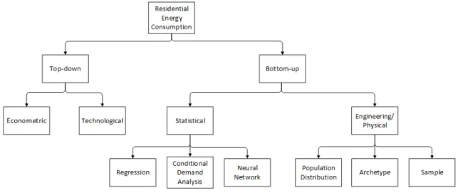
characteristics of the building (e.g. geometry, insulation materials), appliances, occupancy, climate and billing data. As a consequence, these models are seen as a way to evaluate the most cost-effective options to achieve given carbon dioxide targets and to identify areas of improvement. However, this approach makes use of much more data than the top-down models and the energy estimates can be more complex [2]. Since the presented work as the goal of providing consumers with a tool to estimate the energy consumed/generated at their homes, a bottom-up approach provides more accurate information and helps the user implementing techniques of demand response. Therefore, the simulator presented in this document relies on a bottom-up approach.

2.2 Bottom-up models

In order to implement a bottom-up approach there are two main distinct methods that can be used to estimate energy consumption:

1. Statistical methods (SM);

2. Engineering methods (EM).

These models are capable of estimating the contribution of each device towards the aggregate energy balance of a residential building using different data inputs and methods.

The SM are based on historical consumption data, such as billing information, which is then used to regress the energy consumed as a function of a house’s characteristics. Even though this method can be used to model residential energy consumption, it does not take into consideration physical characteristics of the building, such as geometry, the insulation materials used and thermodynamic principles (e.g. heat transfer) and it is not capable of providing information regarding the energy generated by domestic renewable energy generators, such as wind turbines and photovoltaic panels. For that purpose other techniques, such as EM must be considered. However, SM are able to discern the effect of occupant behavior, which has been found to vary widely [6].

EM are based on physical characteristics, such as building’s geometry, insulation, thermodynamics and heat transfer analysis. Therefore, they are able to estimate energy demand/on-site generation without any historical energy information, which makes possible to adapt each estimate to a certain household. As a result, this method is more flexible than SM since it makes it easier to model new devices in which there is very little or no historical consumption data. However, this model cannot provide information regarding occupancy. Each one of the presented models, SM and EM can use different methods to estimate the energy consumption and on-site generation. Figure 2.1 presents the most well documented methods that are commonly used [6].

(27)

2.2. BOTTOM-UP MODELS

Figure 2.1: Possible modeling techniques to estimate the residential energy consumption. Adapted from [6].

2.2.1 Statistical methods

Statistical methods rely on information, such as energy bills, weather records and energy price to make it possible to estimate the energy consumption as a function of house characteristics. So it is possible to relate the collected information with a particular residential building in which the energy balance is intended to be estimated. Moreover, based on the collected information these methods are also capable of estimating the building’s occupant behavior. Bellow, there will be presented three of the best well-documented methods.

2.2.1.1 Regression

This method uses regression analysis to estimate the aggregate energy consumption of the building as a function of some parameters that can affect the energy consumption. The model is evaluated on goodness of fit using the correlation coefficient. Regression analysis can be used both for estimating the use of appliances and to estimate the corre-lation between energy consumption and other factors (e.g. socio-economical). Therefore, through the years a variety of authors have done studies that not only estimate the energy consumption of a household but also estimate the impact of climate, demographics and energy price (Fung et. al [7]) to detect opportunities for energy improvement (Raffio et al. [8]) or to better understand the relationship between them and the energy consumption (Chen et al. [9]).

(28)

the winter and from 838 households through the summer. With this study the authors were able to measure the impact that each factor has on the energy consumption, which is mainly influenced by socio-economic patterns (up to 28.8%), income (18%) and floor area (44%).

Min et al. [10] have used a regression-based statistical analysis for modeling residential energy consumption in the United States (US). For that purpose, data collected from the US Energy Information Administration on the Residential Energy Consumption Survey have been used. By using an ordinary least square method it was possible to find linear and log-linear models for estimating the energy consumption of space heating/cooling, water heating and other appliances. The proposed models have been tested using data from the U.S. Census 2000 and the correlation coefficients for linear/log-linear models were the following 0.594/0.825 (heating), 0.490/0.703 (cooling), 0.295/0.343 (water heating) and 0.409/0.518 (other appliances).

However, in both above mentioned studies authors claimed the need for more data in order to better estimate the power consumed by each appliance. For instance, Chen et al. were not able to isolate the heating/cooling energy consumption from other end-uses. Min et al. have stated that the major limitation was the fact that it was not possible to access a dataset with the tracks of monthly energy end uses.

2.2.1.2 Conditional demand analysis

Conditional demand analysis (CDA) performs regression based on the presence of end-use appliances, by regressing total energy consumption onto the list of owned appliances. One of the biggest advantages of this method is that it only needs information from the user regarding the respective appliances and the energy billing data. On the down side, it requires a huge amount of data from different houses in order to produce reliable results, since it relies on the differences in ownership to determine each appliance’s component of the total dwelling consumption. According to [6] conditional demand analysis was pioneered by Parti and Parti on a study made in 1980 [11]. In that study information from more than 5000 households in San Diego including appliances, occupancy and the billing data was collected. Based on that information Parti and Parti were able to propose a conditional demand regression that considers appliance ownership and the interrelation between those and the building’s characteristics (e.g. floor area) and demographic factors, as shown in Table 2.1.

During the development of this study, authors have specified some conditions in order to limit the use of certain appliances with the intent of determining the regression coefficient. As a consequence, some appliances, such as the air conditioning (AC) and space heating have been disallowed during the periods November - March (for the cooling air conditioning) and July – August (in the case of space heating). The authors have also identified that some appliances have more impact on the energy consumption. For instance: the air conditioning, space heating, water heating, dishwasher, cooking range,

(29)

dryer, refrigerators and freezers play a big role in the load profile of the residential sector. To evaluate the goodness of fitness of this model, the correlation coefficient has been calculated, which has resulted in values ranging from 0.58 to 0.65.

Table 2.1: Interrelation between appliances and the building’s characteristics [11].

Appliances and equipment Interaction variables

Number of occupants

Electricity price

Household

income Floor area

Heating/cooling per unit area

Common appliances X X X

Refrigerator X

Hot water X X X

Space

heating and cooling X X X X

When comparing this method to EM the authors have realized that the presented model is capable of estimating occupant behavior more accurately than the estimates made by the EM, which uses theoretical considerations. Moreover, through this study, the authors have also stated that the use of CDA is beneficial when disaggregating the energy consumption by end-use without sub-metering and the inclusion of behavioral aspects within the coefficients.

Therefore, it is possible to conclude that CDA methods do offer a certain level of detail, which allows not only to estimate the energy consumption of an end-user but also to relate economic and demographic factors with the energy use. However, due to the lack of information regarding the use of new devices it is not capable of modeling more recent technologies, such as solar and wind based generation devices.

Since then, researchers have tried to make improvements so that estimations would be more accurate. Some authors have raised the number of samples; for instance LaFrance and Perron [12] have increased the amount of samples to 100000 homes over the period of 3 years. This increase has resulted in a correlation coefficient value ranging between 0.55 and 0.70. Moreover, they were also capable of identifying strong relationships between incentive activities and appliance penetration. However, the authors weren’t able to separate the energy consumed for refrigeration from that consumed by small appliances, due to lack of information regarding the technical characteristics of the devices used in each home.

2.2.1.3 Neural network

(30)

as much information in the beginning and can be easily adaptable to the addition of new information. According to [13] the use of NN to model the energy consumption of a building has started in the 1990s, beginning with commercial buildings and progressing in complexity.

It has been reported by Krarti et al. [14] that Kreider [15] were the first to apply a NN model to predict the energy consumption of a building, in 1991. This model was built in order to estimate the electricity consumption of a commercial building and the results showed that the predictions of the NN model were accurate. The authors indicated that NN were easier to use than classical regression methods since it learns from fact patterns and there was no requirement for an a priori statistical analysis.

However, the use of NN based methods to model residential energy have been his-torically limited, possibly due to the computational and data requirements or the lack of physical significance of the coefficients relating dwelling characteristics to total energy consumption [6]. On the other hand, they are highly suitable for determining relationships amongst a large number of parameters. Therefore, and because of their simplicity, accuracy and ability to model nonlinear processes (e.g. energy building loads) NN are used for prediction problems as a substitute for other statistical approaches for estimating national end-use energy consumption and the impact of socio-economic factors in the residential sector. But, when compared to other SM, NN are not flexible evaluating the impact of energy conservation measures [15]. Mihalakakou et al. [16] have created an energy model for a residential building in Greece in which they have used a feedforward backpropa-gation NN. The developed model considers the atmospheric conditions, including air temperature and solar radiation. This model has been trained using information regarding energy consumption data that has been collected for the period of five years. Final results were excellent on hourly basis, due to the amount of data used to calibrate the model. The correlation coefficients vary from 0.96 to 0.94, depending on the tested month. Therefore, it is possible to consider that the presented approach can be used to simulate and estimate the energy consumption time series with sufficient accuracy. However, it is not always possible to predict future values of ambient air temperature and total solar radiation. As a consequence, authors have concentrated the estimations in summer months since during this period the Mediterranean has a more predictable weather.

2.2.1.4 Richardson’s model

When designing the simulator it has been adopted a model to generate the data that was not possible to express by using EM, such as occupancy and human habits related with energy consumption. In [5] it is presented a model developed by Richardson et al. that generates synthetic active occupancy data and appliance usage data (including mean power consumption and working period) with a 1min time resolution for a 24-h period, based upon survey data on how people spend their time at home in the United Kingdom (UK) [17] and nationwide ownership statistics. The survey data has been made by using

(31)

many thousands of 1-day diaries recorded at a 10-min resolution.

By integrating the UK statistics with a first order Markov-Chain technique authors were able to make a model that generates synthetic demand data that is only dependent on the tasks performed previously by the user together with the probabilities of the user performing a different task. These probabilities are calculated considering the number of active occupants (inhabitants that are at home and awake), month of the year, type of day (weekend day or week day), the time of the day and meteorological conditions. Therefore, in order to better adjust the simulation to a certain dwelling the user must provide information regarding the number of inhabitants and month, as well as type of the day. Moreover, it considers the sharing of appliances, such as lighting. For example, doubling the number of active occupants in a house is unlikely to double the lighting demand, since occupants will share lighting in common rooms. Although this fact might be true, the model considers that sharing is dependent on the number of active occupants in a house at a given time but also on the appliance type in question. In the case of lightning this model not only considers the human habits and occupancy but also the level of solar radiation, which means that as the solar radiation decreases the lights tend to be switched on (unless there is not any active occupant).

When generating the data the start state is chosen by picking a random number of active occupants from a probability distribution (according to the number of inhabitants set by the user). Subsequent states in the chain are determined by picking a random number for each time step and using this with the appropriate transition probability matrix (given the type of day and the total number of residents in the house). Therefore, each run of this model is different because of the random numbers used in the stochastic generation but all runs are based on the same transition probability matrices and thus exhibit similar characteristics. To validate this model, the authors have recorded data from 22 dwellings around the town of Loughborough (UK) with a time resolution of 1min, in 2008. After comparing both the synthetic and the recorded data it has been found that results were very similar.

2.2.2 Engineering methods

EM are based on physical characteristics, such as building’s geometry, insulation mate-rials, thermodynamics and heat transfer analysis. Methods that can be used in order to estimate energy consumption and on-site generation of renewable energy generators are presented below.

2.2.2.1 Distribution

(32)

appliance it is possible to aggregate those consumptions in order to estimate the residential energy consumption of a bigger region (e.g. city, country). Despite the fact that this method relies on national balance of appliance penetration and might use historical information, it can be considered a bottom-up approach due to its level of disaggregation, as the number of houses and appliance distributions are known. The distribution method has been used in order to model the energy consumption of the residential sector in a variety of countries, such as Italy (Capaso et al. [18]), Canada (Jaccard and Baille [19]), Malaysia (Saidur et al. [20]).

The study made by Capaso et al. has allowed modeling the residential sector based on distributions, which have been determined by using surveys. This data allowed to combine demographic and lifestyle information with engineering models of a wide range of appliances. The developed model was then applied to that region and compared with load recordings.

Saidur et al. created a residential energy model to represent the energy consumption in Malaysia. The presented model is designed based on the distribution estimates of appliances’ ownership made by different researchers, as well as appliances’ power rate and efficiency and appliance use. Due to the Malaysia’s climate, space heating equipment does not need to be considered. The national energy estimate was then calculated by summing the energy of each device. With this model they were also able to measure the overall efficiency of appliances, which was 70%.

2.2.2.2 Sample

Sample methods make use of real house samples, which makes it more accurate when it comes to model a region’s energy consumption since it can realistically reflect the high degree of variety found in actual housing stock, but on the other hand, there is more data to be processed.

Larsen and Nesbakken [21] developed a model of the Norway’s housing stock using information collected from 2013 dwellings. By doing so, they were able to account for every end-use. When compared to CDA, it has been pointed out as a main advantage the fact that this method is more accurate in considering the impact of new technologies. Griffith and Crawley [22] have done a similar study using 5430 buildings, however in both studies the authors have stated that one of the disadvantages of this method was the amount of input data, which requires a significant computing capability.

2.2.2.3 Archetypes

The archetypes are considered to be a restricted number of residential buildings which together represent the different classes of houses found in the residential sector. To generate these archetypes certain characteristics must be considered, such as geometry, thermal characteristics and operating parameters. Although, this methods can be more accurate

(33)

than statistical ones when estimating the energy consumption of each device, its lack of information regarding occupancy can lead to misleading estimations [2].

Shimoda et al. [23] developed a residential end-use energy consumption model on the city scale for Osaka, Japan. They developed 20 dwelling types and 23 occupant types to represent the variety of houses within the city. For each type of building conductive heat transfer analysis were considered when modeling. However, it has been considered that insulation materials were identical to the materials available in 1997. The occupants’ model types were developed based on the number of family members, appliance ownership levels and appliance ratings.

MacGregor et al. [24] developed a residential model using a total of 27 archetypes. In order to estimate the energy consumption of each archetype, they used typical values of occupancy, appliances and lightning to run an hourly analysis program. Energy con-sumption values were then extrapolated to provincial levels based on the total number of dwellings represented by each archetype. Final results were then compared to top-down estimates and were found to be in agreement.

During the analysis of these two studies it was possible to identify that the use of archetypes has some advantages when compared to other EM. For instance, when compared to the distribution method, this model allows capturing the interconnectiv-ity between appliances and end-uses. Secondly, when compared to the sample method archetypes reduce the simulation time, since the number of archetypes is limited. However, this method provides a more limited representation of the housing sector and, similar to the other EM, it requires the assumption of occupancy values.

2.2.3 Hybrid models

Hybrid models are a combination of both engineering and statistical methods and can use any of the different methods of each model. This approach makes possible to correlate the data that is better estimated by each one of those methods, as shown in the examples mentioned next. For instance, it is possible to improve the information provided when using EM by adding information regarding the building’s occupancy, which can only be estimated using SM otherwise a constant value would have to be assumed.

The Canadian Hybrid Residential End-use Energy and Emission Model (CHREM) is based on two modeling components, statistical and physical that are used to make estimates on the energy consumption of the major end-use groups: domestic appliances and lightning, domestic hot water and space heating/cooling. The statistical part of the model is employed by using NN to estimate the annual energy consumption for appliances, lightning and domestic hot water, since these devices are predominantly influenced by occupant behavior. On the other hand, estimates on space heating/cooling are made possible through the use of a building performance simulation package, which makes possible to consider the use of new technologies [25].

(34)

estimates. In this study, the authors have treated the information from the engineering ap-proach as prior evidence on usage patterns for specific appliances, and by using Bayesian analysis, engineering estimates were integrated into CDA model to estimate hourly ap-pliance consumption. The sample data contained daily electric consumption information (excluding weekends) and appliance ownership information from 129 households that had been collected for two summer months in 1977, in Los Angeles. The engineering estimates were generated from a simulation program and include estimates of occupant behavior. This simulation program includes twelve scenarios, which represented three types of buildings (single family detached, single family attached and multifamily), two weather districts, and two building sizes. Average loads for each of these appliances of the sample data were constructed using a weighted average of the twelve scenarios, where the weights reflected the housing type and size characteristics of the sample, and the distribution of the sample households between the weather districts. For central air conditioning, both methods provided similar estimates, but for dishwasher the estimates differed considerably, since dishwasher consumption was more dependent on consumer behavior, which is more difficult to predict using EM.

In this thesis an agent-based simulator based on a hybrid bottom-up approach, com-bines a synthetic data generator (to represent statistical methods) with engineering meth-ods. The fact that the presented work is not a model itself, but a simulator that allows the users to estimate the energy demand and on-site generation of their homes, makes it a more extensible and operable tool for the end-user. The synthetic data generator that has been used was designed by Richardson et al. [5] and provides information regarding occupancy and power consumption of each electrical device, including lightning, which are more dependent on the user interaction. EM were considered to model the physi-cal behavior of some devices, i.e. the electric water heater, air-conditioning, refrigerator, photovoltaic panel and wind turbine.

(35)

C

H

A

P

T

E

R

3

M

ODELING THE SIMULATOR

This chapter presents the modeling techniques used to provide to the user estimates regarding the demand and on-site generation of its residential building. Apart from these estimates, the developed simulator should also feature the following characteristics: add/remove devices in real time (during the simulation period), adjust each simulation to the user’s necessities and suggest ways of maximizing the use of the energy produced on site and reduce the cost of the energy imported from the grid.

To accommodate these specifications this simulator has been made using an agent-based modular architecture, allowing therefore the user to change the simulation’s condi-tions in real time and making possible the exchange of information between the different devices. Moreover, it allows the integration of different data sources, such as meteorologi-cal data and energy prices. To module the behavior of each device it has been used either, thermal/electric models or Richardson’s model, depending on the device. At last, this simulator uses genetic algorithms to provide suggestions on load optimization. The user interaction as been made possible through the use of a graphical interface that enables the user to adjust each simulation and beware of the estimates made, which are displayed through the use of charts.

3.1 Functional model

(36)

CHAPTER 3. MODELING THE SIMULATOR

Figure 3.1: Features the simulator has available to the user.

After initiating the simulation process the user has the ability of adding/removing any device, as well as configuring any of them with the intended specifications. It is important to mention that any of these changes to the device’s characteristics can be made in real time, during the simulation process. Despite the fact that the simulation represents a 24-h period, it is possible for the user to adjust the time scale in order to make the simulation run at the desired speed. For instance, the user can set that 1min in the simulation represents 0.3 s in the real world, which means that the 24-h period will take 7 min and 12 seconds to be simulated.

On the output, this simulator provides information about the energy consumption/-generation, including the working period and the energy produced/consumed by each device, as well as the total energy balance of the home. Moreover, information regarding the energy cost is provided at the end of the simulation period, as well as suggestions on how to maximize the use of the renewable energy produced in the building and on how to lower the energy cost.

3.2 Architecture

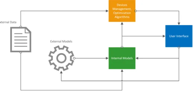
In order to implement the features presented in section 3.1 an architecture containing five major entities has been designed. Each one of them is composed of at least one module that is responsible for implementing the functionalities of the entity it is associated with. Moreover, it is also important to assure the interoperability between modules, to enable the exchange of information among entities. Figure 3.2 represents these entities, as well as the data flux (symbolized by the arrows).

(37)

3.2. ARCHITECTURE

Figure 3.2: System’s architecture.

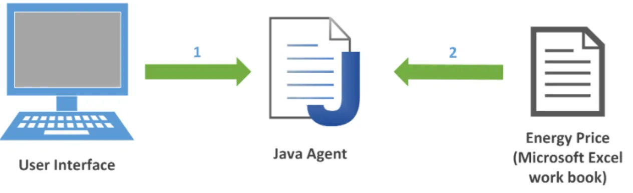
The "External Data" entity is composed by two modules, including the Microsoft Excel work book with the meteorological data and another one with the energy prices (as shown in Figure 3.3). Meteorological data is important not only to estimate the power generated by the renewable energy generators (photovoltaic panel and wind turbine) but also to estimate the power consumption of the thermostat-controlled appliances (e.g. refrigerator). Therefore, it is important to make this information available to the entities in which it is estimated the power consumed/produced by each device. The energy price is used to estimate the cost of each simulation.

"External Models" incorporates the Richardson’s model, which is responsible for providing estimates of the occupancy schedules and the power consumed by the event-driven appliances (household appliances that are only dependent on the human interaction to change their status, e.g. washing machine). Since these estimates depend on information provided by the user, it should receive data from the "User Interface" and send the estimates made to the “Internal Models” entity so they can be interpreted.

(38)

to receive the data set by the user.

"User Interface" entity is composed of just one module capable of providing the user a way of adjusting the simulation to the respective needs. Thus, it is possible to provide a good level of abstraction so that a deep knowledge on the devices is not required when setting up a new simulation. On the output, the user interface displays charts with the variation of power consumption and on-site generation, as well as the temperature variance of the thermostat-controlled appliances, the estimated occupancy schedules and the total cost of the energy consumed from the grid.

All of the information, regarding energy demand/on-site generation is then saved on the entity named "Devices Management, Optimization Algorithms", which is also responsible for calculating the energy cost of each simulation and provide suggestions on load optimization, so it would be possible to maximize the use of the energy produced on site and lower the energy bill.

Figure 3.3: Modules that integrate the different entities.

To make possible the implementation of the system presented in Figure 3.2 and the interaction between the different modules in Figure 3.3 this simulator has been designed using an agent-based modular architecture. This approach not only allows the creation of various independent modules (agents) but it also makes their interaction possible through the exchange of messages. Therefore, modularity offers some characteristics that this simulator can benefit from. For instance, it is possible to divide the data that needs to be processed among the existing modules, it is easily scalable (more agents can be add without compromising the existing architecture) and it is adaptable to changes. This makes possible to separate the various algorithms that estimate the behavior of the devices, making a certain agent responsible for estimating the behavior of just one device. Even though the algorithms are separated, it is possible for one device to react to another one change in behavior through the messages exchanged. Moreover, due to the fact that each module is independent from the others it is possible, during the simulation process, to

(39)

3.3. OPTIMIZATION ALGORITHMS

add/remove devices in real time without compromising the rest of the estimates that are being made for other devices. It is also possible to add various instances of the same device enabling, for example, to have more than one television or air-conditioning.

3.3 Optimization algorithms

Optimization algorithms were added to the system so it would be possible to provide suggestions to the user on how to maximize the use of the energy produced on site and lower the energy cost, by rescheduling the use of certain appliances. For this purpose genetic algorithms (GA) were implemented due to the fact they can handle complicated op-timization problems with nonlinear, discrete and constrained search spaces [27], providing good solutions using few computational resources.

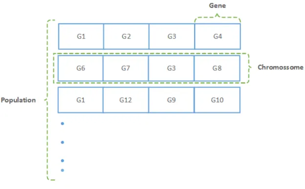
GA provide a method of solving optimization problems by imitating the evolutionary process based on the mechanics of Darwin’s natural selection. To the group of existing indi-viduals it is given the name of "population" (i.e. possible solutions). As in the evolution of organisms, each individual’s information is described by sign rows called "chromosomes". Each of these chromosomes has then a number of "genes" containing a possible solution, as shown in Figure 3.4. It is important to mention that different chromosomes can have equal genes in their constitution.

Figure 3.4: Illustration of the constitution of a GA’s population.

(40)

process such as selection, crossover, and mutations to each individual within the pop-ulation and the subsequent fitness (objective function) of each individual is calculated for evaluation. The individual with the highest fitness value of all the enquired indi-viduals becomes the optimum individual. However, because the size of the population and the number of possible generations is restricted the final solution presented by the algorithm might not be the optimal solution, since that restriction comprises the capability of evaluating all the possible cases.

3.3.1 Energy consumption optimization

The optimization of the energy consumption has been built so that the user can maximize the use of the renewable energy produced in the building. Consequently, by using this algorithm it is possible to know how to shift the working period of the controllable appliances to the times where there is more energy available. To make it possible, this algorithm must find a solution that reduces as much as possible the difference between the power generated and consumed in every minute of the 24-h period, as it is expressed in equation (3.1).

Min

(

N

∑

t=0

|Pprod(t)−Pcons(t)|

)

(3.1)

In (3.1), Nis the number of minutes of a day, 1440 min. Pprod and Pcons are the pro-duced and consumed power, respectively, at timet. To implement this fitness function,

information regarding the working period and power demand/on-site generation of each device must be known.

3.3.2 Energy cost optimization

The optimization of the energy cost has been built so that the user could not only maximize the use of the renewable energy produced in the building but also reduce the energy cost. This optimization algorithm is similar to the one in section 3.3.1 but it also considers the price of the energy that needs to be consumed from the grid when the amount of renewable energy available is not enough to satisfy the building’s demand. In those cases it suggests shifting the use of controllable appliances to the times the user can save more money, as expressed in equation (3.2).

Min

(

N

∑

t=0 C(t)

)

, where

C(t) =

(

Eprice(t)∗(Pcons(t)−Pprod(t)), if Pcons(t)>Pprod(t) 0, if Pcons(t)≤ Pprod(t)

(3.2)

In (3.2), Nis the number of minutes of a day, 1440 min. Pprod and Pcons are the pro-duced and consumed power, respectively, at timet. To implement this fitness function,

(41)

3.3. OPTIMIZATION ALGORITHMS

information regarding the working period and power consumption/ on-site generation of each device must be known, as well as the energy price (Eprice).

3.3.3 Adaptation of the genetic algorithms to the simulator

For this simulator it has been considered that in order to have the least interference on the user’s comfort only the washing machine, washer dryer and the dish washer could be time-shifted. Moreover, it has been assumed that these devices would not work more than once a day, which results in having just three genes per chromosome (each one representing a different controllable appliance). These genes contain information on the time at which each appliance could start working, which can be at any time betweent=0 min andt=1440−∆_work(where∆_workis the working period of the device).

(42)

Figure 3.5: Flowchart of the GA’s operation.

(43)

C

H

A

P

T

E

R

4

I

MPLEMENTING THE SIMULATOR

4.1 Technology used

In order to implement an agent-based modular architecture, the Java Agent DEvelop-ment Framework (JADE) has been used and the communication between agents was made possible thanks to Foundation for Intelligent Physical Agents Communication Language (FIPA-ACL). As a consequence, the majority of the simulator was designed in Java, using NetBeans Integrated Development Environment (IDE). This IDE has been selected due to the fact that it is open-source, supports Java and provides tools that allow the design of a user interface.

To integrate the simulator with Richardson’s model it has been built a Visual Basic program to run the existing macros in the Microsoft Excel work book. For this purpose Notepad++ has been used. The thermal and electric models presented in section 4.4 were tested before used in this simulator by using Matlab software.

4.2 Detailed architecture

(44)

CHAPTER 4. IMPLEMENTING THE SIMULATOR

Figure 4.1: Detailed architecture of the simulator.

4.3 Input data

The simulator was designed so that data from different sources could be used. In this specific case, data sources include: meteorological data (saved on a Microsoft Excel document), energy price, Richardson’s model and the data provided by the user using the graphical interface. However, due to the modular structure of the simulator this data sources could be replaced. For instance the simulator could collect data directly from a meteorological station instead of using data previously measured and Richardson’s model could be replaced by a similar model.

4.3.1 Information set by the user

Through the user interface it is possible to add different types of devices with different specifications. Table 4.1 presents the different devices’ types that the simulator has avail-able for the user, as well as the data that must be provided when adding new appliances or energy generators to the simulation.

(45)

4.3. INPUT DATA

some of the devices that have more impact on the energy demand of the Portuguese resi-dential sector are the refrigerator, washing machine, clothes dryer, dishwasher, lightning, hot water heating, air heating/cooling systems and oven, as shown in Figure 4.2.

Table 4.1: Types of devices the simulator has available.

Type of devices Input data

Photovoltaic panel Area of the panel Wind turbine Diameter of the turbine Refrigerator Mean power

Temperature range

Water heater

Mean power Temperature range Water flow

Temperature of the inlet water Air conditioning Mean power

Temperature range Oven and television Mean power Washing machine

Washer dryer and Dishwasher

Mean power

Duration of the washing period

Figure 4.2: Devices that have the most impact on the Portuguese energy demand of the residential sector [28].

(46)

approach, it would have been possible to make different types of devices available to the user without changing the simulator’s architecture. Due to this modular architecture, the system also allows the user to add as many instances of the same device with different specifications as needed. Moreover, when setting a new simulation the user is also able to make configurations regarding the number of inhabitants, month of the year, type of day and the simulation speed.

4.3.2 Meteorological data

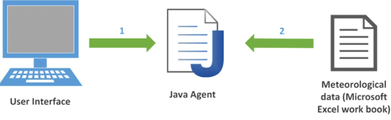
Due to the fact that electricity consumption and generation in residential households varies significantly depending on seasonality [29], when simulating the behavior of both the thermostat-controlled appliances and the renewable energy generators, the simu-lator makes use of meteorological data that has been acquired using a meteorological station installed on the Department of Electrical Engineering at New University of Lisbon (38°39’38.2"N 9°12’17.6"W) during a one year period with a time resolution of 1-min. These measurements include the outside temperature, solar radiation and wind speed averaged during a 1-month period to produce a typical day for each of the 12 months considered. As a result, when setting up a new simulation, the user can choose the month of interest. Since, the meteorological data has been saved on a Microsoft Excel work book a Java agent is used to enable the interaction between the simulator and the data file. Therefore, after the user has set the month of interest (using the user interface) that information is sent to the Java agent so that it can then read the meteorological data of the correspondent month from the Microsoft Excel work book. This interaction is presented in Figure 4.3.

Figure 4.3: Interaction between the meteorological-data’s file and the simulator.

4.3.3 Energy price

The total cost of the imported energy, purchased from the electrical grid when the energy produced on-site is not sufficient to satisfy the building’s demand, is calculated at the end of each simulation by using the prices of the tri-hourly tariff for a low special tension on a diary cycle of a Portuguese electricity supplier (Energias De Portugal). The

(47)

4.3. INPUT DATA

energy price within this tariff varies depending on the time of the day and the season of the year, as it is depicted in Figure 4.4 and 4.5.

This information together with the estimation of the energy demand and on-site generation makes possible to introduce more control and flexibility on the demand side (i.e. the user is now aware of the impact that each device has on the load curve and the cost associated with it). Therefore, it is possible for the user to implement demand response techniques, by rescheduling the time at which a specific device operates, in order to reduce the energy cost and maximize the use of renewable energy, as suggested by the optimization algorithms (sections 3.3.1 and 3.3.2).

Figure 4.4: Energy prices for winter months (from October to March).

Figure 4.5: Energy prices for summer months (from April to September).

(48)

Figure 4.6: Interaction between the energy-price’s file and the simulator.

4.4 Used models

The implementation of the EM has been made by using both thermal and electrical models to describe the behavior of the thermostat-controlled appliances and the energy generators, respectively.

4.4.1 Thermal models

4.4.1.1 Building

When studying the thermodynamics of a residential building certain assumptions have been made. For instance, it has been considered that only the outside temperature and the air conditioning are capable of altering the inside temperature of the house. Consequently, the house’s thermal mass is limited to the thermal mass of the air. Secondly, in this model the building is viewed as a single space where the circulation effects are neglected and it is assumed that the inside temperature is uniform. The model used to calculate the building’s inside temperature (Ti+1) is based on the one proposed by [30] and has the mathematical formula shown in (4.1).

Ti+1 =εTi+ (1+ε)

T0±ηqi A

(+:heating,−:cooling) (4.1) In (4.1),Ti is the temperature inside the residential building at the instantti. At the instantti = 0 min the inside temperature is considered to be equal to the value of the outside temperature (for that same time).T0varies according to the data in the data base,

which has the measured meteorological information.ηrepresents the thermal conversion

efficiency when the air conditioning is heating. On the other hand, when cooling it repre-sents the coefficient of performance. Andqi is the power delivered by the air conditioning to the building. Insulation (A), as well as the inertia factor (ǫ) are calculated through the

formulas presented in (4.2) and (4.3), respectively.

In equation (4.2),mcis the average thermal mass,τis the time interval betweenti and

(49)

4.4. USED MODELS

the surface area,xis the width of the insulation layer andkis the thermal conductivity of

the material used to isolate.

ε=e−mcτA (4.2)

A= Sk

x (4.3)

When starting a new simulation a building with the characteristics presented in Table 4.2 is assumed by default. These characteristics were given as an example, but could have been defined differently.

Table 4.2: Characteristics of the building used in the simulator.

Building’s characteristics

Volume of the building 1247 m3

Walls’ area 320 m2

Roof’s area 601 m2

Number of windows 6

Windows’ size 1(m)x1(m)

Windows’ glass thickness 0.015 m

Walls’ thickness 0.2 m

Windows’ thermal conductivity 0.780 W/(m°C) Walls’ thermal conductivity 0.038 W/(m°C) Roof’s thermal conductivity 0.038 W/(m°C)

(50)

Figure 4.7: Variation of the temperature inside the house with the status of the air condi-tioning.

4.4.1.2 Refrigerator

The model used to calculate the refrigerator’s inner temperature (Ti+1) is based on the one proposed by [31] and has the mathematical formula shown in (4.4):

Ti+1= εTi+ (1+ε)

T0−ηqi A

(4.4) In (4.4),Ti is the refrigerator/freezer inner temperature at timeti. Parameterqidenotes the electrical power required to turn on the compressor andηis the efficiency of the cooling

device.T0describes the ambient temperature, which varies according to the house’s inner

temperature and it is calculated using the formula presented in (4.1). The system’s inertia (ǫ) depends upon the insulation (A), whose equations are both presented in (4.2) and

(4.3), respectively.Srepresents the surface area andxis the width of the insulation layer. kis the thermal conductivity of the material used to isolate. Equation (4.4) could also

be used to model the temperature of a freezer. To model the refrigerator’s behavior the following assumptions have been made, according to [31]: the thermal conductivity is always constant and has the value of 3.21 W/(m°C), the coefficient of performance (η)

is 3.0 and the thermal mass is equally distributed along the refrigerator/freezer’s inner compartment and is equal to 19.95 kWh/°C.

The model presented in (4.4) was implemented using Matlab software, considering the assumptions presented before. Moreover, it has been considered a constant outside tem-perature of 20 °C and a mean power of 70 W. It has also been defined that the temtem-perature

(51)

4.4. USED MODELS

of the refrigerator’s inner compartment should not exceed 8 °C nor be lower than 4 °C. The results obtained are presented in Figure 4.8, where it is possible to see the variation of the temperature inside the refrigerator together with the power consumption.

Figure 4.8: Variation of the temperature inside the refrigerator with the status of the compressor.

4.4.1.3 Electrical water heater

According to [32] the electric water heater can be modeled based on energy flow analysis and the temperature of the water inside the tank can be obtained as a function of time, as shown in (4.5).

Th(t) =Th(τ)nGR′Tout+BR ′

Tin+QR ′o h

1−e−RC1(t−τ)

i

(4.5)

In (4.5),Th(t)is the water’s temperature inside the tank at timet.Tinis the incoming cold water temperature andToutis the ambient temperature of the house, as shown in Figure 4.9). The temperature of the house is not considered constant and is given by the equation in (4.1).τis the initial time andTh(τ)is the temperature of the water in that instant. However, each time thatQorFchangesτis restarted. As a result,τgets the value

(52)

Figure 4.9: Representation of the water tank.

The insulation characteristics of the water heater are given by R (tank insulation thermal resistance).Pis the heating element power and must be set inkW. The electric

energy input (Q) is calculated trough (4.6).

Q=3, 4121.103P (4.6)

The constantCis calculated using the formula in (4.7).

C= ρVCp (4.7)

In (4.7),Vis the volume of the water tank,Cpis the specific heat of water andρthe density of water.G,BandR′are defined according to the formulas shown in (4.8), (4.9)

and (4.10), respectively. In (4.8),SAis the surface are of the water tank and in (4.9)Fis the

water flow rate.

G= SA

R (4.8)

B= FρCp (4.9)

R′ = 1

G+B (4.10)

When the user adds an electrical water heater to its simulation it has the characteristics presented in Table 4.3 by default. These characteristics were given as an example, but could have been defined differently.

Before implementing the model described by equation (4.5) in the simulator it has been tested using Matlab software. For that purpose a script has been built to represent the behavior of the electrical water heater. This script considers the characteristics in Table 4.3. However, it has been considered a constant outside temperature of 20 °C, a water flow of 0.0016 m3_{/h and 15 °C as the temperature of the incoming cold water. Moreover,} it has been defined that the temperature of the water inside the tank should not exceed 55 °C and nor be lower than 50 °C. The results obtained are presented below in Figure

(53)

4.4. USED MODELS

4.10, where it is possible so see the variation of the temperature inside the water tank as a function of the power consumed by the device. In this example it has been considered a mean power of 4.5 kW.

Table 4.3: Characteristics of the water tank used in the simulator.

Water-tank’s characteristics

Volume 1.13 m3

High 1.79 m2

Radius 0.45 m

Area 2.01 m

Insulation thermal resistance 2.642 (°C.m2_)/W

Figure 4.10: Variation of the water’s temperature inside the water tank with the power consumption.

4.4.2 Electric models

4.4.2.1 Photovoltaic panel

(54)

consider the effect of the ambient temperature.

Preal =SηA₁₀₀₀S (1+ (Tcell−25)γ) (4.11) In (4.11),Srepresents the solar radiation andAis the photovoltaic panel area, which

can be set by the user during the simulation period. The efficiency of the photovoltaic panel is given byηandγis the temperature factor for power (-0.005 °C−1<γ<-0.003 °C−1_{) [33].}_T

cell is the cell’s temperature and can be calculated using the formula shown in (4.12).

Tcell =Tamb+ NOCT

−20

800 S (4.12)

In 4.12, Tamb is the ambient temperature and NOCT is the Normal Operating Cell Temperature which is a characteristic of the solar panel. The ambient temperature, as well as the solar radiation are not constant and depend upon the data in the meteorological data base.

When the user adds a photovoltaic panel to the simulation it has the characteristics presented in Table 4.4 by default. These characteristics were given as an example, but could have been defined differently.

Table 4.4: Characteristics of the photovoltaic panel used in the simulator.

Photovoltaic-panel’s characteristics

NOCT 45 °C

η 15%

γ -0.0035 °C−1

4.4.2.2 Wind generator

According to [34], the amount of power that can be absorbed by a wind turbine is given by the model in (4.13).

P= 1

2CpρairAv3 (4.13)

In (4.13),Cpis the power coefficient and is calculated using the formula shown in (4.14). The power coefficient represents the aerodynamic efficiency of the wind turbine. Because of the Betz limit, theCpvalue cannot be higher than 16/27 [35].ρairis the air density,Ais the swept area of the turbine andvis the wind velocity, which is not constant and varies

according to the data on the meteorological data base.

Cp=0, 5176

"

116 1

λ−0,08β −

0,035

β3+1

−0, 4β−5

#

e −21 1

λ−0,08β−0,035β3 ₊0, 068_λ (4.14)

(55)

4.4. USED MODELS

For this kind of turbine (horizontal axis wind turbine),Cphas a value between 0.2 and 0.5 [36].βis the incident blade angle and is the tip speed ratio, which is given by (4.15).

λ= rΩr

v (4.15)

The turbine radius is given by r and can be set by the user during the simulation

period.Ω_ris the rotational frequency of the turbine andvis the wind speed.

When the user adds a wind turbine to the simulation it has the characteristics presented in Table 4.5 by default. These characteristics were given as an example, but could have been defined differently.

Table 4.5: Characteristics of the wind turbine used in the simulator.

Wind-turbine’s characteristics

Ω_r 45 °C

Cp 0.4

4.4.3 Richardson’s model

In the case of event-driven appliances (e.g. electrical oven) their status are dependent on the user’s interaction along the day, turning them on and off. As a consequence, the behavior of these appliances is associated with occupancy schedules and human habits, which cannot be estimated using EM. By integrating Richardson’s model in the simulator it makes possible to provide estimates regarding occupancy schedules and human habits, thereby enabling the working time and power consumption of the event-driven appliances to be estimated. Additionally, occupancy schedules are also used to help estimating the status of the air conditioning, since it is considered that it only works when the building has at least one active occupant (an individual that is at home and awake) and the temperature is out of the comfort range, defined previously by the user. However, in order to make this estimates possible the user must provide information regarding the month of the year, number of inhabitants, type of day and the appliances which consumption is intended to be estimated. Figure 4.11 illustrates the data input and output of the Richardson’s model.