Faculdade de Ciências e Tecnologia
Departamento de Informática
Dissertação de Mestrado
Mestrado em Engenharia Informática
Solving Colored Nonograms
Luís Pedro Canas Ferreira Mingote
(aluno nº 29634)
Faculdade de Ciências e Tecnologia
Departamento de Informática
Dissertação de Mestrado
Solving Colored Nonograms
Luís Pedro Canas Ferreira Mingote
(aluno nº 29634)
Orientador:
Prof. Doutor Francisco de Azevedo
Trabalho apresentado no âmbito do Mestrado em Engen-haria Informática, como requisito parcial para obtenção do grau de Mestre em Engenharia Informática.
To my wife Marta. Without her incentive, support, patience, inspiration and family dedica-tion I could never have finished this work.
To my daughters Margarida and Matilde. That this work may be an incentive to always seek to increase their knowledge.
I would like to thank Prof. Francisco de Azevedo for his time and orientation. I cannot thank him enough for all the patience in reading, understanding and proposing improvements to my writings.
I also would like to thank Prof. Paula Amaral, from the Mathematics Department, for mak-ing available CPLEX for testmak-ing.
Thank you Alberto Bigotte de Almeida for all your support and help in the beginning of this endeavor.
I would also like to thank all my family for their support and incentive.
I would like to thank my late mother, Maria do Céu, for the education she gave me and for instilling the will to always be a better person and always widen my knowledge.
I would also like to remember my late grandfather who played a significant role in my education.
Nesta dissertação aprofundamos o estudo da resolução de nonogramas coloridos utilizando Programação Linear Inteira (PLI). As formas conhecidas de resolução deste tipo de problemas são a força-bruta, o método iterativo e PLI.
A nossa aproximação generaliza a utilizada por Robert A. Bosch desenvolvida para, apenas, nonogramas a preto e branco, tornando assim disponível uma solução nova e universal para a resolução de nonogramas utilizando PLI.
Sendo as implementações do método iterativo as que apresentam melhores resultados ao nível do desempenho, desenvolvemos também um método híbrido que combina esta aproxi-mação e PLI.
Estes puzzles têm, muitas vezes, várias soluções. A forma de as encontrar pelo modo iter-ativo é uma pesquisa em árvore com retrocesso. De forma a encontrar as restantes soluções na nossa aproximação aplicamos um algoritmo que utiliza um corte binário para excluir soluções já conhecidas.
Para efeito de testes comparativos entre as diversas aproximações ao problema, desenvolve-mos um gerador de nonogramas que permite definir a resolução do puzzle, o seu número de cores e a densidade (número de células pintadas vs. resolução).
Finalmente comparamos o desempenho da nossa aproximação para resolver nonogramas coloridos com o da aproximação interativa.
Palavras-chave: Nonograma, pintar-por-números, PLI, Programação Linear Inteira
In this thesis we deepen the study of colored nonogram solving using Integer Linear Pro-gramming (ILP). The known methods for solving this kind of problems are the depth-first search (brute-force) one, the iterative one and the ILP one.
Our approach generalizes the one used by Robert A. Bosch which was developed for black and white nonograms only, thus providing a new universal solution for solving nonograms using ILP.
Since the iterative implementations are the ones that present better performance results, we also developed a hybrid method that combines this approach and the ILP one.
These puzzles often have more than one solution. The way to find them using the iterative method is to make a tree search with backtracking. In order to find the remaining solutions using our approach, it is necessary to apply an algorithm that uses a binary cut to exclude already known solutions.
In order to perform comparative tests between approaches, we developed a nonogram gen-erator that allows us to define the resolution of the puzzle, its number of colors and its density (number of painted cells vs. resolution).
Finally we compare the performance of our approach in solving colored nonograms against the iterative one.
Keywords: Nonogram, paint-by-numbers, ILP, Integer Linear Programming
1 Introduction 1
1.1 Context 1
1.2 Problem Description 1
1.2.1 Initial problems 1
1.2.2 Nonograms 1
1.2.2.1 Black and White Nonograms 2
1.2.2.2 Colored Nonograms 2
1.3 Scope of work and main contributions 3
1.4 Document’s structure 4
2 Nonograms 5
2.1 Black and white Nonograms 5
2.1.1 Simple boxes 6
2.1.2 Punctuating 7
2.1.3 Simple spaces 8
2.1.4 Mercury 9
2.1.5 Forcing 9
2.1.6 Glue 9
2.1.7 Joining and splitting 10
2.2 Colored Nonograms 11
2.2.1 Simple boxes 12
2.2.2 Punctuating 14
2.2.3 Simple spaces 14
2.2.4 Mercury 15
2.2.5 Forcing 15
2.2.6 Glue 16
2.2.7 Joining and splitting 16
2.3 Approaches to solving Nonograms 17
2.3.1 Depth-first search (brute-force) 18
2.3.2 Iterative approach 19
2.3.3 Integer Linear Programming approach 21
3 An ILP model for solving Colored Nonograms 23
3.1 Model Description 23
3.1.1 Notation 23
3.1.2 Variables 24
3.1.3 Block constraints 25
3.1.4 Double Coverage Constraints 26
4.1 Pure ILP approach 33
4.2 Nonogram Generator 34
4.3 Hybrid ILP approach 36
5 Conclusions and Future Work 45
A Full Results 47
B Results by block density 59
C Objective function constraint results 63
C.1 Graphic Analysis 63
C.2 Full Results 64
D Nonogram File Formats 71
D.1 Bosch based file format 71
D.2 Olšák file format 76
1.1 Black and white nonogram example (unsolved: left, solved: right) 2 1.2 Colored Nonogram Example - "Fall" from [2] 3
2.1 Black and white nonogram example 6
2.2 Example for the method Simple boxes in black and white nonograms 7
2.3 Example for the method Punctuating 8
2.4 Example 1 for the method Simple spaces applied to a black and white nonogram 8 2.5 Example 2 for the method Simple spaces applied to a black and white nonogram 8
2.6 Example for the method Mercury 9
2.7 Example for the method Forcing 10
2.8 Example for the method Glue 10
2.9 Example for the method Joining and splitting applied to a black and white
nono-gram 10
2.10 Solving a black and white Nonogram Example 11 2.11 Solving a black and white Nonogram Example — after last (horizontal) iteration 12 2.12 Example 1 for the method Simple boxes 13
2.13 Example for the method Punctuating 14
2.14 Example 1 for the method Simple spaces 14 2.15 Example 2 for the method Simple spaces 15
2.16 Example for the method Mercury 15
2.17 Example for the method Forcing 16
2.18 Example for the method Glue 16
2.19 Example for the method Joining and splitting 17 2.20 Solving a Colored Nonogram Example — "Fall" from [2] 17 2.21 Solving a Colored Nonogram Example — "Fall" from [2] 18 2.22 Solving a Colored Nonogram Example — "Fall" from [2] — After final
(hori-zontal) iteration 19
2.23 Depth-first search — all possibilities for a line 20
4.1 Generated nonogram 35
4.2 ILP: Average resolution by density (20x20) and number of solved puzzles 39 4.3 Iterative: Average resolution by density (20x20) and number of solved puzzles 39 4.4 ILP: Average resolution by density (40x60) and number of solved puzzles 40 4.5 Iterative: Average resolution by density (40x60) and number of solved puzzles 41 4.6 ILP: Average resolution by density (100x100) and number of solved puzzles 41 4.7 Iterative: Average resolution by density (100x100) and number of solved puzzles 42 4.8 Hybrid ILP vs. Pure ILP comparison (20x20) 43 B.1 ILP: Average resolution time by block density, in seconds (20x20) 59
2.1 Experimental Results (in seconds) 21
4.1 Experimental Results (in seconds) 33
4.2 Results of adding equation (4.1) to ILP (in seconds) 34 4.3 Number of solved puzzles by method and dimension 37 4.4 Number of solved puzzles by method, dimension and density 37 4.5 Number of solved puzzles by method and density 38 4.6 Average time to solve a puzzle by dimension 38 4.7 Average time to solve a puzzle by density 38
A.1 Full Results (in seconds) 48
C.1 Objective Function Constraint Full Results (in seconds) 64
1.1
Context
The work hereby presented was developed during the Master Program in Computer Sci-ence Engineering (Bologna second cycle), under the original theme "Solving Problems from CSPLib".
1.2
Problem Description
1.2.1 Initial problems
Initially, the purpose of this work was to solve problems from CSPLib (www.csplib.org), a known library of problems for modeling and solving. Given the lack of knowledge about the majority of the existing problems and our interest in exploring and solving new problems, thus broadening our knowledge base, we decided to analyze the following five:
• prob012: Nonograms • prob020: Darts tournament • prob022: Bus driver scheduling • prob032: Maximum density still life • prob037: Peg solitaire
Although some work was done on problem "prob032 - Maximum density still life", specifi-cally the implementation of the Bucket Elimination algorithm by [11], we decided to deepen the study about problem "prob012 - Nonograms" since it appeared to us that there were approaches that had not been explored, specially to what concerns colored nonograms.
1.2.2 Nonograms
Nonograms are a popular kind of puzzle whose name varies from country to country, includ-ing Paint by Numbers and Griddlers. The goal is to fill cells of a grid in a way that contiguous blocks of the same color satisfy the clues, or restrictions, of each line or column.
According to Wikipedia [21], these kind of puzzles were created in 1987 by Non Ishida, a Japanese graphics editor, and Tetsuya Nishio, a professional Japanese puzzler, at the same time and with no relation whatsoever. Soon after, nonograms started appearing in Japanese puzzle magazines and later as electronic games. Today, magazines with nonogram puzzles are published in several countries and are available as electronic games in a variety of platforms.
left, solved, to the right).
Figure 1.1 Black and white nonogram example (unsolved: left, solved: right)
Known approaches to solving black and white nonograms are the depth-first search (brute-force) one, the iterative one, the ILP one by Bosch [7] and a genetic algorithm by Wouter Wiggers [20].
1.2.2.2 Colored Nonograms
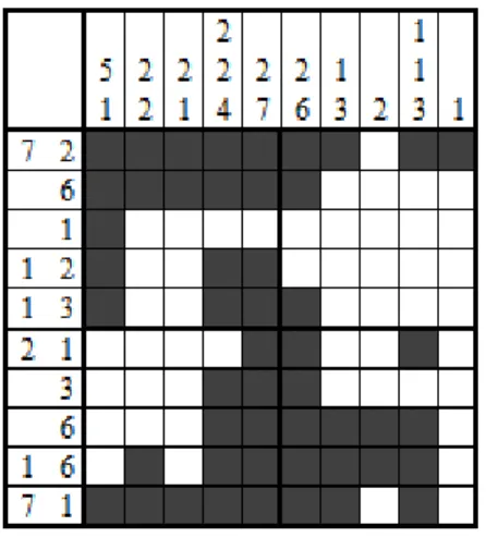
In colored nonograms the clues are composed of pairs that indicate the size and color of each sequence of blocks to be filled. For example, the clue <(3,Red), (1,Green), (2,Blue)>
in a sequence must always be separated by at least one empty cell. Figure 1.2 represents an example of a colored nonogram with 10 lines by 8 columns with 3 colors.
Figure 1.2 Colored Nonogram Example - "Fall" from [2]
1.3
Scope of work and main contributions
Within the scope of this work, colored nonograms were studied in order to develop an Integer Linear Programming model for solving them. This model is based on the one provided by Bosch in [7] for black and white nonograms and generalizes it so it can solve both black and white and colored puzzles. Bosch’s file format was also adapted to colored nonograms and our implementation also supports lines with no clues.
Since the iterative approach is the one that presents the best results, according to Jan Wolter in [23] and according to the tests we performed (shown ahead), we decided to build an hybrid model that integrates both approaches.
In order to compare results of both our models and the iterative one, we built a nonogram generator that can generate puzzles given a resolution (width×height), a number of colors and a density (global or by color).
• An ILP model for solving colored nonograms; • A nonogram instance generator;
• An hybrid implementation between the iterative approach and our ILP approach for col-ored nonogram solving.
• A more systematic study of the different nonogram solving approaches
• An adaptation of an algorithm that obtains multiple solutions to an ILP problem, with a simplification that makes it more efficient to specific problems
1.4
Document’s structure
This document is organized in the following way: In Chapter 2 nonograms (both black and white and colored) are described in full and the best known approaches are detailed.
In Chapter 3 the ILP model we developed to solve colored nonograms is described, includ-ing a demonstration that this model corresponds to the one by Bosch in [7] for black and white nonograms. It is also shown how to apply a simple technique in order to find additional solu-tions in case the first solution obtained for a puzzle is not unique. A description of the hybrid approach between the iterative approach and the hereby presented ILP model is also described. In Chapter 4 results from the presented solutions are compared to its iterative counterpart. A description of the nonogram generator is also presented.
In Chapter 5 the results of the previous chapter are analyzed and the conclusions of this work are presented. We also suggest some future work based on the one presented here.
In the previous chapter a brief description of nonograms was presented. In this one a more detailed explanation about nonograms is shown.
Nonograms are a popular kind of puzzle whose name varies from country to country, including Paint by Numbers and Griddlers. The goal is to fill cells of a grid in a way that contiguous blocks of the same color satisfy the clues, or restrictions, of each line or column.
According to Wikipedia [21], these kind of puzzles were created in 1987 by Non Ishida, a Japanese graphics editor, and Tetsuya Nishio, a professional Japanese puzzler, at the same time and with no relation whatsoever. Soon after, nonograms started appearing in Japanese puzzle magazines and later as electronic games. Today, magazines with nonogram puzzles are published in several countries and are available as electronic games in a variety of platforms.
The most common nonograms are black and white, but they exist also in colors. In fact, black and white nonograms are a specialization of colored nonograms, i.e., are two colored nonograms.
Also there is a different kind of nonogram — calledtriddlers— in which cells are triangles. In this kind of puzzles we have three sets of clues instead of only two. These puzzles can also exist in multiple colors.
Ueda e Nagao prove in [19] that the nonogram problem is NP-Complete.
2.1
Black and white Nonograms
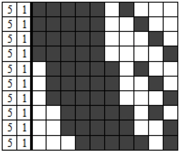
In black and white nonograms the clues indicate the sequence of contiguous blocks of cells to be filled (e.g. the clue 3,1,2 indicates that there is a block of 3 contiguous cells, followed by a sequence of one or more empty cells, then a block of one cell filled, followed by another sequence of one or more empty cells, finally followed by a sequence of two filled cells in that row or column). Figure 1.1 shows an example of a black and white nonogram (unsolved, to the left, solved, to the right).
According to Wikipedia [21], in order to solve this kind of puzzle it is necessary to determine which cells will be filled (black) and which will be empty (white). Determining which cells will be empty is as important as determining which will be filled because the former will help delimiting the solutions for the blocks of each line or column1.
Simpler puzzles, like the one shown in figure 2.10, can usually be solved by applying the following methods to each line at a time.
1For the sake of simplicity, from this point forward, only lines will be mentioned, since the reasoning is the
same for columns.
Figure 2.1 Black and white nonogram example
2.1.1 Simple boxes
At the beginning of the solution, when there are no filled cells, for each blockbi∈ {b1, ...,bB}in
each row, the space availableS(bi) for it is determined, assuming that the remaining blocks are
moved closer to the extremities of the grid as possible (previous blocks to the left and subsequent block to the right). bi represents a set of filled cells in sequence (vector). The value forS(bi)
can be calculated using equation 2.1, whereL represents the size of the line, Brepresents the number of blocks on the line andT(bi) represents the size ofbi.
S(bi)=L−B+1− B
X
k,i
T(bk) (2.1)
It is also possible to know for each block what is the potential first cell that it can occupy through equation 2.2, wherebi[1] is block’sbifirst cell position in the grid.
bi[1]=
(
1 ; i=1
be determined for blockbi.
T(si)=2T(bi)−S(bi) (2.3)
In the same way, it is possible to obtain the first cell (consequently the remaining) of this sub-block through equation 2.4, wheresi[1] is the position of the first cell of sub-blocksi.
si[1]=bi[1]+S(bi)−T(bi) ; T(si)>0 (2.4)
Figure 2.2 Example for the method Simple boxes in black and white nonograms
As an example, for the 10th line of the puzzle shown in figure 2.1,L=10,B=2,T(b1)=7 and T(b2)= 1. Therefore the space available for the first block isS(b1)= 10−2+1−1=8 andS(b2)=10−2+1−7=2. The leftmost indexes each can occupy areb1[1]=1 andb2[1]=
1+7+1=9.
As for the sub-blocks of cells that can be filled at this point, T(s1)= 2×7−8 =6 and T(s2)=2×1−2= 0, i.e., it is not possible to fill, for now, any cell in respect to the second block, but it is possible to fill six cells with respect to the first one. It is yet to determine the starting cell of the first and second sub-blocks: s1[1]=1+8−7=2, i.e., it is possible to fill, at this point, cells 2 through 7 of that line.
Figure 2.2, from line 10 of the puzzle shown in figure 2.1, exemplifies this method for a size 10 line with with two blocks of sizes 7 and 1.
2.1.2 Punctuating
In order to solve the puzzle it is also very important to enclose with empty cells the extrem-ities of each completed block, immediately, as described in the methodSimple spaces. Precise punctuating usually leads to moreForcingand can be vital to finishing the puzzle.
Figure 2.3 Example for the method Punctuating
2.1.3 Simple spaces
The purpose of this method is to find cells that can not be filled by any block due to the constraints imposed by filled cells. For example, a block that is already complete may have at least an empty cell to its left and at least another one to its right, unless it is adjacent to the beginning or the end of the line.
Figure 2.4 from column 8 of the puzzle shown in figure 2.1 shows an example of this method.
Figure 2.4 Example 1 for the method Simple spaces applied to a black and white nonogram
In figure 2.5, based on one from Wikipedia, a more illustrative example of this method is shown.
Figure 2.5 Example 2 for the method Simple spaces applied to a black and white nonogram
expand between the second and the sixth cell because it has to include the fourth cell. This means that cells 1 and 7 will be empty.
2.1.4 Mercury
Mercuryis a special case ofSimple spaces. The name comes from the way mercury pulls back from the sides of a container.
If there is a filled cell on a line that is at the same distance from the border as the size of the first block, then the first cell has to be empty. This is true because the first block would not fit to the left of the filled cell. It will have to spread through that cell leaving the first cell behind. Besides, when the cell is in reality a set with cells more to the right, there will be more spaces at the beginning of the line, determined by applying this method several times.
In figure 2.6, from Wikipedia, an example of this method is shown.
Figure 2.6 Example for the method Mercury
2.1.5 Forcing
In this method the importance of empty cells is demonstrated. An empty cell in the middle of an incomplete line can force a block to complete itself to one of the sides of the empty cell.
In figure 2.7, from line 8 of the puzzle shown in figure 2.1, an example of this method is shown.
2.1.6 Glue
In this method a full cell at the beginning (or the end) of the possible space for a block forces the completion of that block to the empty side. In the same way, an empty cell in the middle of the possible space for a block can condition the placement of that block’s cells.
Figure 2.7 Example for the method Forcing
Figure 2.8 Example for the method Glue
In this case, the filled cell in position 1 indicates that the size 5 block has to fill cells 1 through 5. Since the block becomes complete, we mark cell 6 of that column as empty through method punctuating.
2.1.7 Joining and splitting
Filled cells nearby one another can be united or separated according with the number and size of that line’s blocks. In this case the whole line has to be analyzed together with the information available for every block.
In figure 2.9, from Wikipedia, an example of this method is shown.
Figure 2.9 Example for the method Joining and splitting applied to a black and white nonogram
Using these methods we can easily solve these more simple puzzles. Figures 2.10(a) through 2.11 show the two horizontal iterations and the vertical one made in order to solve the puzzle shown in figure 2.1.
(a) After first horizontal iteration (b) After first vertical iteration
Figure 2.10 Solving a black and white Nonogram Example
2.2
Colored Nonograms
In colored nonograms the clues are composed of pairs that indicate the size and color of each sequence of blocks to be filled. For example, the clue <(3,Red), (1,Green), (2,Blue)>
indicates that there is a block of 3 contiguous cells of red, followed by a block of one green cell separated or not by a sequence of empty cells, followed by a sequence of two blue cells separated or not from the green block by a sequence of empty cells, in that row or column. The general rule for separating blocks is that if a block is of the same color of the previous one in the respective sequence then they must be separated by at least an empty cell. Otherwise (i.e., the two blocks have different colors), they may have no cells in between, i.e., they may be adjoining blocks. Note that in the particular case of black and white nonograms this means that blocks in a sequence must always be separated by at least one empty cell. Figure 1.2 represents an example of a colored nonogram with 10 lines by 8 columns with 3 colors.
In the same way as black and white nonograms, in order to solve this kind of puzzle it is necessary to determine which cells will be filled (colored) and which will be empty (white). Determining which cells will be empty is as important as determining which will be filled because the former will help delimiting the solutions for the blocks of each line or column.
Figure 2.11 Solving a black and white Nonogram Example — after last (horizontal) iteration
two colored nonograms). In that way, the same methods, with some nuances, can be applied to colored nonograms, each line at a time, in order to solve them.
These methods are explained again, but now applied to colored nonograms.
2.2.1 Simple boxes
At the beginning of the solution, when there are no filled cells, for each blockbi∈ {b1, ...,bB}in
each row, the space availableS(bi) for it is determined, assuming that the remaining blocks are
moved closer to the extremities of the grid as possible (previous blocks to the left and subsequent block to the right). bi represents a set of filled cells in sequence (vector). The value forS(bi)
can be calculated using equation 2.5, whereL represents the size of the line, Prepresents the number of pairs of contiguous blocks of the same color on the line andT(bi) represents the size
ofbi.
S(bi)=L−P− B
X
k,i
T(bk) (2.5)
For black and white nonograms equation 2.5 becomes equation 2.1 where B represents the number of blocks on the line.
It is also possible to know for each block what is the potential first cell that it can occupy through equation 2.7, wherebi[1] is block’s bifirst cell position in the grid and f is a function
that returns 1 if the blocks are of the same color and 0 otherwise (see equation 2.6 whereCbi is the color of blocki).
f(bi,bj)=
(
0 ;Cbi,Cbj 1 ;Cbi=Cbj
bi[1]=
(
1 ; i=1
bi−1[1]+T(bi−1)+ f(bi,bi−1) ; i>1 (2.7) For black and white nonograms f always returns 1 and equation 2.7 becomes equation 2.2. Within this set of cells it is possible to determine which subset is actually filled by analyzing the extremities of the solution, i.e., sliding the block as far to the left as possible and then as far to the right as possible and checking which cells are common to both solutions. In this way, equation 2.8 gives the size of this sub-block, whereT(si) is the size of the sub-blocksithat can
be determined for blockbi.
T(si)=2T(bi)−S(bi) (2.8)
In the same way, it is possible to obtain the first cell (consequently the remaining) of this sub-block through equation 2.9, wheresi[1] is the position of the first cell of sub-blocksi.
si[1]=bi[1]+S(bi)−T(bi) ; T(si)>0 (2.9)
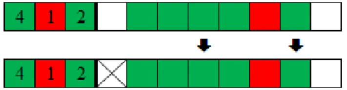
Figure 2.12 Example 1 for the method Simple boxes
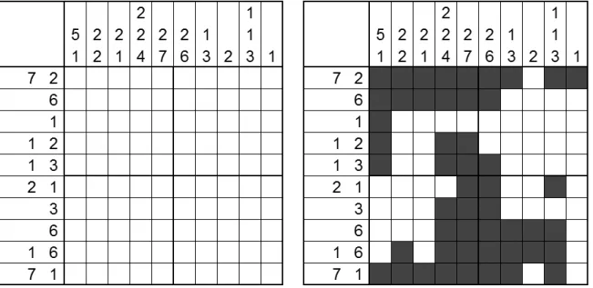
As an example, for the fourth line of the puzzle shown in figure 1.2, L=8, P=0, B=4, T(b1)=3,T(b2)=2, T(b3)=1 andT(b4)=1. Therefore the space available for the first block isS(b1)=8−0−4=4, S(b2)=8−0−5=3, S(b3)=8−0−6=2 andS(b4)=8−0−6=2. The leftmost indexes each can occupy areb1[1]=1,b2[1]=1+3+0=4,b3[1]=4+2+0=6 andb4[1]=6+1+0=7.
As for the sub-blocks of cells that can be filled at this point, T(s1)=2×3−4=2,T(s2)=
Figure 2.13 Example for the method Punctuating
2.2.3 Simple spaces
The purpose of this method is to find cells that can not be filled by any block due to the constraints imposed by filled cells. For example, a block that is already complete may have at least an empty cell to its left and at least another one to its right, unless it is adjacent to the beginning or the end of the line.
Figure 2.14 from line 2 of the puzzle shown in figure 1.2 shows an example of this method.
Figure 2.14 Example 1 for the method Simple spaces
In figure 2.15, based on one from Wikipedia, a more illustrative example of this method is shown.
Figure 2.15 Example 2 for the method Simple spaces
2.2.4 Mercury
Mercury is a special case ofSimple spaces. The name comes from the way mercury pulls back from the sides of a container.
If there is a filled cell on a line that is at the same distance from the border as the size of the first block, then the first cell has to be empty. This is true because the first block would not fit to the left of the filled cell. It will have to spread through that cell leaving the first cell behind. Besides, when the cell is in reality a set with cells more to the right, there will be more spaces at the beginning of the line, determined by applying this method several times.
In figure 2.16, from line 1 of the puzzle shown in figure 1.2, an example of this method is shown.
Figure 2.16 Example for the method Mercury
2.2.5 Forcing
In this method the importance of empty cells is demonstrated. An empty cell in the middle of an incomplete line can force a block to complete itself to one of the sides of the empty cell.
Figure 2.17 Example for the method Forcing
the last three cells of the line. Applying method Simple boxes to both blocks turns out to fill cells 2, 3 and 9.
2.2.6 Glue
In this method a full cell at the beginning (or the end) of the possible space for a block forces the completion of that block to the empty side. In the same way, an empty cell in the middle of the possible space for a block can condition the placement of that block’s cells.
In figure 2.18, from column 5 of the puzzle shown in figure 1.2, an example of this method is shown.
Figure 2.18 Example for the method Glue
In this case, filled brown cell in position 4 preceded by filled green cell in position 3 indicates that the size 7 brown block has to fill cells 5 through 10.
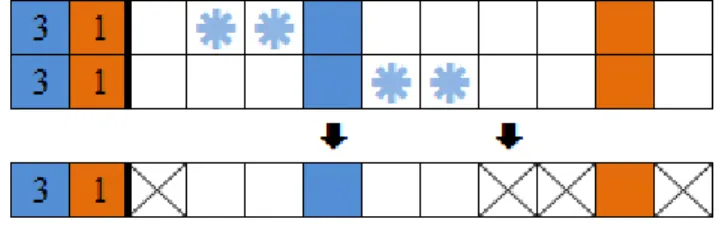
2.2.7 Joining and splitting
Filled cells nearby one another can be united or separated according with the number and size of that line’s blocks. In this case the whole line has to be analyzed together with the information available for every block.
In figure 2.19, from column 2 of the puzzle shown in figure 1.2, an example of this method is shown.
Figure 2.19 Example for the method Joining and splitting
Using these methods one can easily solve these more simple puzzles. Figures 2.20(a) through 2.22 show the three horizontal iterations and the two vertical ones made in order to solve the puzzle shown in figure 1.2.
(a) After first horizontal iteration (b) After first vertical iteration
Figure 2.20 Solving a Colored Nonogram Example — "Fall" from [2]
2.3
Approaches to solving Nonograms
(a) After second horizontal iteration (b) After second vertical iteration
Figure 2.21 Solving a Colored Nonogram Example — "Fall" from [2]
we will reach another state where another guess must be made to continue to try to solve the puzzle, and so on. If a contradiction is reached, then the value we chose for a determined cell is wrong. In black and white puzzles this means that the cell will have the opposite value (empty if the chosen value was filled, filled otherwise), but in colored nonograms another color can be chosen for that cell. These more complex puzzles are usually difficult to solve by a human.
This is where computer based approaches can be useful.
Known approaches for solving nonograms are the depth-first search (brute-force), the it-erative approach and the ILP approach. A comparison between a genetic algorithm and the depth-first search algorithm, by Wouter Wiggers [20], was also found. As mentioned in the article, the genetic algorithm not always reaches a solution, however it reaches a near solution very quickly.
2.3.1 Depth-first search (brute-force)
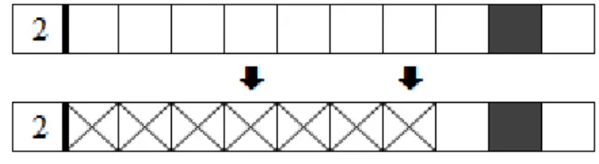
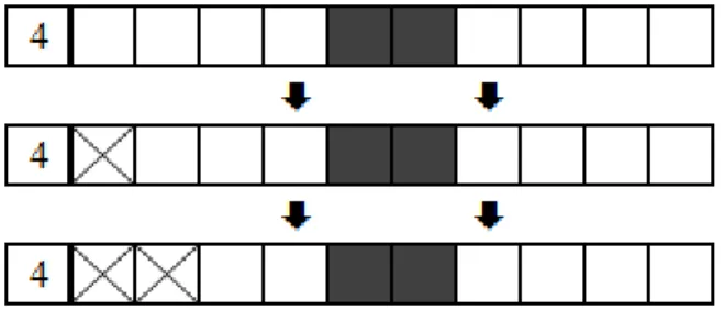
This approach tries all possible combinations for the set of blocks of each line. For example, for a size 10 line, belonging to a black and white nonogram, with two blocks of sizes 5 and 1, we would have 10 possibilities only for that line, as shown in figure 2.23.
An optimization of this algorithm is to begin with the lines that have fewer possibilities. However, if we want to find all solutions then all possibilities must be explored.
Figure 2.22 Solving a Colored Nonogram Example — "Fall" from [2] — After final (horizontal) itera-tion
• P-99: Ninety-Nine Prolog Problems [10]
• Colin Barker’s Home Page - LPA Win-Prolog Goodies [6] These implementations only work for black and white nonograms.
2.3.2 Iterative approach
The iterative technique consists in determining, for every line, cyclically, which cells can be considered filled and which cells can be considered empty, in accordance to the information available at the moment, until a solution is reached or no more cells can be determined.
To find this information an algorithm is applied to each line at a time. This algorithm is called aline-solver. A line-solver is an algorithm that given a single line (row or column), and the state of that line so far, tries to figure out what additional cells can be marked.
When the successive application of theline-solverstops contributing to the puzzle’s resolu-tion, the search for contradictions can help.
This method includes:
1. Forcing an unknown cell to be empty or full;
2. Reapply the methods mentioned in order to find a solution;
Figure 2.23 Depth-first search — all possibilities for a line
The problem to this method is the choice of a cell to try a contradiction, i.e., having an heuristic to find the best cells to try a value. Besides, while trying a cell for a contradiction another situation may arise in that another try to find a contradiction must take place, and so forth.
Usually, the best cells to initiate a contradiction try are the following: • Cells that have many filled neighbors;
• Cells near the border or nearby sets of empty cells;
• Cells that are between lines that consist of more empty cells.
Steven Simpson, in his site [16], describes his algorithm for the resolution of nonograms. As mentioned above, the algorithm tries to solve, or partially solve, a line for each iteration. The order in which lines are tried to be solved is defined by the value of equation 2.10, whereB is the number of blocks of that line,Lis the size of the line andT(b1) toT(bB) are the sizes of
each block. When non-negative, the result is the number of filled cells that can be determined from an empty line. A negative value indicates a shortfall of pre-determined cells. Note that whenB=1 andT(bi)=LthenI=Land this is the maximum value.
I=(B+1)
B
X
i=1
T(bi)+B(B−L−1) (2.10)
Exceptionally, if B=0 (empty line) thenI=L.
Table 2.1 Experimental Results (in seconds)
Puzzle R×C×Col NPC Brute-force (Prolog) Brute-force opt (Prolog) Iterative ILP
Fall 10x8x3 47 1,050.70 0.03 0.07 0.03
Fish 16x16x2 164 (timeout) 0.08 0.07 0.21
AtoZ 16x16x2 50 (timeout) 0.92 0.10 23.04
Time 35x30x5 520 (timeout) (out of memory) 0.21 3.51
order, i.e, higher ranked line-solvers are only applied after lower ranked ones don’t reveal more cells. There are four well-known line-solvers: fast, complete, olsak[13] and fcomp. The first gets most of the information available; the second gets everything logically deductible, but is very inefficient; the third is a variation of the first one, but is a little more exhaustive and gets all the information; the fourth is a revised version of the second one, but is significantly more efficient.
In [23], Jan Wolter compares several nonogram solvers in which the best three (Wolter’s pbnsolve[22], Simpson’snonogram[15] and Olšák’sgrid [13]) use one or more of these line-solvers. Simpson’ is the only that does not solve colored nonograms.
2.3.3 Integer Linear Programming approach
Robert A. Bosch [7] presented in 2001 a solution based on Integer Linear Programming as well as the code that converts the definition of a puzzle in a program that can be used by CPLEX [3] to solve the puzzle.
The mentioned program only works for puzzles that have clues for all the lines.
Since this approach only solves black and white nonograms we proposed to develop an ILP model that solves colored nonograms.
The performance results of our approach compared to an adaptation for colored nonograms of the depth-first search provided by Hett [10], an adapted version of the optimized depth-first search approach also by Hett and Olšák’sgridare shown in table 2.1.
The times were measured on a 2.4 GHz Intel©Centrino©vPro™with 2 GB of RAM running Microsoft© Windows©. The Prolog program was run in ECLiPSe [1] and the generated ILP problems were run on SCIP [4]. Results are shown in table 4.1, where NPC stands for "Number of Painted Cells". The time limit imposed was 30 minutes.
Given the good performance of the iterative approaches we also proposed to develop a hy-brid model between this approach and the ILP one.
The ILP approach presented here starts from scratch with an empty grid and, in general, could not improve the Iterative method for the available tests, although already presented similar results using a non commercial tool.
In the previous chapter we verified that no ILP model for solving colored nonograms exists. In this chapter we describe the model we developed for this purpose.
3.1
Model Description
As in [7], our approach is to think of a colored nonogram as a problem comprised of two interlocking tiling problems: one involving the placement of the row blocks, and the other involving the placement of the column blocks. If a cell is painted (it can be assumed that unpainted cells are painted white) then it must be covered by both a row block and a column block; if it is painted white (not painted) then it must be left uncovered by the row blocks and the column blocks.
3.1.1 Notation
The notation used here is similar to the one used by Bosch in [7], as follows. m=the number of rows,
n=the number of columns,
o= the number of colors excluding white (We use a sequence of natural numbers to identify colors, starting at 1 (1,2, . . . ,o).),
bri =the number of blocks in rowi, 1≤i≤m, bcj=the number of blocks in column j, 1≤ j≤n, sri,1,sri,2, . . . ,sri,br
i
=the block-size sequence for rowi, scj,1,scj,2, . . . ,scj,bc
j
=the block-size sequence for column j,
cri,1,cri,2, . . . ,cri,br i
=the block-color sequence for rowi, ccj,1,ccj,2, . . . ,ccj,bc
j
=the block-color sequence for column j.
In addition, let
eri,t = the smallest value of j such that row i’s tth block can be placed in rowi with its leftmost pixel occupying cell j,
its topmost pixel occupying celli.
These are constants valid for the empty puzzle. (The letters "e" and "l" stand for "earliest" and "latest"). In our example puzzle, the second row’s first block must be placed so that its leftmost pixel occupies cell 1 or 2, the second block must be placed so that its leftmost pixel occupies cell 5 or 6, and the third block must be placed so that its leftmost pixel occupies cell 6 or 7. In other words
er2,1=1,lr2,1=2,er2,2=5,lr2,2=6,er2,3=6 and lr2,3=7.
These values are obtained by iteratively placing the blocks in their leftmost or topmost possible cells and then placing them in their rightmost or bottommost possible cells. In our example, the first block’s first cell is 1 and, since the first block’s size is 4 and the color of both blocks is different, the second block’s first possible cell is 5. Then, since the color of the third block is also different from the second one and the size of the second block is 1, the third block’s first possible cell is 6. Now, the third block is pushed to its rightmost cell (7) and one finds out that the second block’s last possible cell is 6 and the first block’s last possible cell is 2.
Note that the rules for determining these values are the same for colored or black and white nonograms. Of course, in black and white puzzles all the blocks are of the same color, which means they have to be separated by at least one empty cell.
3.1.2 Variables
As in the approach by Bosch in [7], in our approach there are three sets of variables. One set specifies the color of each cell:
∀1≤i≤m,1≤j≤n zi,j=
c ; if row i’s j
th cell is painted
with colorc(1≤c≤o) 0 ; if row i’s j
th cell is not
painted
(3.1)
The other two sets of variables are concerned with placements of the row and column blocks.
∀1≤i≤m,1≤t≤bri,eri,t≤j≤lir,t yi,t,j=
1
; if rowi’s tth block is placed in rowiwith its leftmost pixel occupying cell j
0 ; if not
∀1≤j≤n,1≤t≤bcj,ecj,t≤i≤lcj,t xj,t,i= 1
; if column j’s tth block is placed in column j with its topmost pixel occupying cell i
0 ; if not
(3.3)
3.1.3 Block constraints
To ensure that rowi’stthblock appears in rowiexactly once, the following imposes
∀1≤i≤m,1≤t≤bri lri,t
X
j=er i,t
yi,t,j=1 (3.4)
For line 2 of our example we have
y2,1,1+y2,1,2=1,
y2,2,5+y2,2,6=1,
y2,3,6+y2,3,7=1.
For the next two sets of constraints the auxiliary function (3.5) is defined. This function, which was already defined as equation 2.6 in chapter 1, returns the value 1 if the two arguments are the same, and 0 otherwise, which will be useful to compare colors of two contiguous blocks.
eq(c1,c2)= (
1 ; ifc1=c2
0 ; otherwise (3.5)
To ensure that row i’s (t+1)th block is placed to the right of its tth block, the following imposes
∀er i,t+1≤j≤l
r
i,t yi,t,j≤
lri,t+1
X
j′=j+sr i,t+eq(c
r i,t,c
r i,t+1)
yi,t+1,j′ (3.6)
In line 2 of our example we have
y2,1,2≤y2,2,6,
y2,2,6≤y2,3,7.
∀ec j,t+1≤i≤l
c
j,t xj,t,i≤
lj,t+1
X
i′=i+sc j,t+eq(c
c j,t,c
c j,t+1)
xj,t+1,i′ (3.8)
3.1.4 Double Coverage Constraints
To guarantee that each painted cell is covered by both a row block and a column block, the following pair of sets of inequalities imposes:
∀1≤i≤m,1≤j≤n zi,j≤ bri
X
t=1
min{lri,t,j} X
j′=max{er i,t,j−s
r i,t+1}
yi,t,j′×cr
i,t (3.9)
∀1≤i≤m,1≤j≤n zi,j≤ bc
j X
t=1
min{lc j,t,i} X
i′=max{ec j,t,i−s
c j,t+1}
xj,t,i′×cc
j,t (3.10)
Without these restrictions the model would allow having cells painted by row blocks, but not painted by any column block, or vice versa. The first set of inequalities (3.9) states that if rowi’s jthcell is painted, then at least one of rowi’s blocks must be placed in such a way that it covers rowi’s jthcell. (The upper and lower limits of the second summation make sure that j′ satisfies the two pairs of sets of inequalitieseri,t≤ j′≤lri,t and j−sri,t+1≤ j′≤ j. The first pair holds if, and only if, rowi’stthcell is covered when rowi’stth block is placed in rowiwith its leftmost pixel occupying cell j′. The second pair holds if and only if rowi’s jthpixel is covered when rowi’stthblock is placed in row iwith its leftmost pixel occupying pixel j′). The other set of inequalities (3.10) makes sure that if rowi’s jthcell is painted, then at least one of column
j’s blocks covers it. For row 2 of our example we have for cellz2,5that
z2,5≤y2,1,2×cr2,1+y2,2,5×c
r
2,2,
z2,5≤x5,1,1×cc5,1+x5,1,2×c
c
5,1
solving, it is kept as a linear inequality. Nevertheless, below it is proven that this is sufficient for a correct and complete model, in the presence of the other sets of constraints.
Finally, constraints that prevent unpainted cells from being covered by the row blocks or column blocks are included — sets of inequalities (3.11) and (3.12).
∀1≤i≤m,1≤j≤n,1≤t≤bri, j−sri,t+1≤j′≤j,er i,t≤j′≤l
r
i,t zi,j≥yi,t,j′×c
r
i,t (3.11)
∀1≤i≤m,1≤j≤n,1≤t≤bcj,ecj,t≤i′≤lc j,t,i−s
c
j,t+1≤i′≤i zi,j≥xj,t,i′×c
c
j,t (3.12)
In line 2 of our example we have
z2,5≥y2,1,2×cr2,1, z2,5≥y2,2,5×c
r
2,2,
z2,5≥x5,1,1×cc5,1, z2,5≥x5,1,2×c
c
5,1.
One might think that it is necessary to ensure that each painted cell must be covered by one row block and one column block of the same color. However, the remaining sets of constraints ensure that there is only the need to guarantee that a painted cell must be covered by one row block and one column block. In order to prove it, let us explore all the possibilities regarding the coverage of some cellz:
1. No block covers cellz;
2. Only one block covers cellzand it is of the same color;
3. Only one block covers cellzand its color is smaller than the color ofz; 4. Only one block covers cellzand its color is greater than the color ofz; 5. More than one block covers cellz;
Of these five possibilities, only the first two are possible in real puzzles. The last three are the ones that our model has to avoid.
In sake of simplicity, but with no loss of generality, only inequality (3.9), for lines, of the double coverage constraints will be used in our case analysis for these five possibilities:
Possibility 1: The only way to satisfy this possibility is with an empty cell z, with value 0, which, by inequality (3.9), will guarantee that no block covers it (forcing the respective yi,t,j′ variables to be 0), i.e.
bri
X
t=1
Max{lr i,t,j} X
j′=Min{er i,t,j−s
r i,t+1}
Possibility 4: In the case that there may be one block that covers cell z, and which color is greater than the color ofz, then inequality (3.9) would be satisfied. However, this would violate inequality (3.11) thus turning the solution invalid.
Possibility 5: If more than one block covers cellz, the set of inequalities (3.9) could only be satisfied if the sum of the colors of the covering blocks is greater than or equal to the color of cellz. But this would violate the set of equations (3.4) thus turning the solution invalid.
3.1.5 Objective Function
Since this is a satisfaction problem there is no need for an objective function, but since ILP solvers need one, the following is included (note that this function is a constant and we already know its value):
minimize/maximize
m
X
i=1
n
X
j=1
zi,j (3.13)
3.1.6 Pre-conditions
We also include in our approach one pre-condition in order to verify whether the puzzle is trivially impossible to solve, before even trying to search for a solution (another improvement with respect to [7]). This is a necessary, but not sufficient condition that will save the time of trying to solve a puzzle that is impossible, and that also helps determining whether there is any error in the definition of the puzzle. This condition, shown by equation (3.14), checks whether the sum of the sizes of all blocks of each color is the same for both the rows and columns clues.
∀c∈{1,...,o}
m
X
i=1
br i X
t=1
f(sri,t,cri,t,c)=
n
X
j=1
bcj
X
t=1
f(scj,t,ccj,t,c) (3.14)
3.2
Instantiation to Black and White Nonograms
Ifois set to 1 (o=1), thus allowing only black and white in a puzzle, our model becomes the one provided by Bosch in [7], i.e., definition (3.1) becomes
zi,j=
(
1 ; if rowi’s jthcell is painted
0 ; if rowi’s jthcell is not painted (3.15) Definitions (3.2) and (3.3) are kept from the approach provided by Bosch. Equation (3.4) is equal to the one in the approach by Bosch, but inequality (3.6) was extended so blockt+1 can follow blocktimmediately, due to possible contiguous blocks of different colors. For black and white puzzles it corresponds exactly to the formulation in [7] since all blocks have the same color which leads theeqfunction to always yield value 1. Inequalities (3.7) and (3.8) are similar, but regard columns. Finally, since the only possible color takes value 1, the double coverage constraints set by the sets of inequalities (3.9) and (3.10) become
∀1≤i≤m,1≤j≤n zi,j≤ bri
X
t=1
min{lri,t,j} X
j′=max{er i,t,j−s
r i,t+1}
yi,t,j′, (3.16)
∀1≤i≤m,1≤j≤n zi,j≤ bcj
X
t=1
min{lcj,t,i} X
i′=max{ec j,t,i−s
c j,t+1}
xj,t,i′, (3.17)
∀1≤i≤m,1≤j≤n,1≤t≤br i,j−s
r
i,t+1≤j′≤j,e r i,t≤j′≤l
r
i,t zi,j≥yi,t,j
′ (3.18)
and
∀1≤i≤m,1≤j≤n,1≤t≤bc j,e
c j,t≤i′≤l
c j,t,i−s
c
j,t+1≤i′≤i zi,j≥ xj,t,i
′ (3.19)
as in [7] (where theminandmaxfunctions are incorrectly swapped in the summation limits).
3.3
Finding Multiple Solutions
The described ILP model allows finding a single solution to a puzzle, which actually is the best one, although in this case all solutions are alike since the optimizing function is a constant.
(i,t,j)∈A (i,t,j)∈B
Basically, after finding a solution to the problem, the constraints in inequality (3.20) are added to the problem and another try is made to find another solution.
3.4
Hybrid model
The hybrid model we propose here basically consists in substituting the search part of the iter-ative approach by our ILP model.
At first, the puzzle is logically solved, i.e., one or moreline-solversare applied to every line of the puzzle, repeatedly, until there is no more information that can be inferred. Then, if the puzzle is not completely solved, the ILP model is instantiated.
Our implementation generates a CPLEX LP file (.lp) that represents the current state of the puzzle according to the model presented in section 3.1. This approach is more flexible than generating the ILP model specifically for a solver like SCIP [4] or CPLEX [3] because it allows the comparison of results between different ILP solvers.
SCIP is currently one of the fastests non-commercial mixed integer programming (MIP) solvers. ILOG CPLEX©is a commercial mathematical programming optimizer that, among other things, solves mixed integer programs. Although SCIP is advertised as the best performing non-commercial MIP solver, CPLEX — the best MIP solver — is five times faster.
The process of instantiating our ILP model, and subsequently generating the LP file, en-volves the following steps:
• Compute earliest and latest constants • Write objective function to file • Write block constraints to file
• Write double coverage constraints to file
• Write bounds to file: here is where the partial solution found by the iterative approach is inserted in the ILP model
Since among the best performing implementations of the iterative approach only pbnsolve and Olšák’s (grid) can solve colored nonograms, we decided to adaptpbnsolveinto our hybrid approach. The reason we did not choose grid was that the program code comments are in Czech. On the other hand, pbnsolve’s code comments are very complete and understandable. Steven Simpson’snonogram[16] can not solve colored nonograms.
In the previous chapter our ILP model for solving colored nonograms was described. We also described an hybrid approach to solving colored nonograms between the iterative and the ILP ones.
Here, we present the results of the performance tests we ran in order to compare the different approaches to solving colored nonograms.
First we present the results between our pure ILP approach and the iterative and the depth-first search ones. Then we show the results obtained by comparing our hybrid approach and the iterative one.
4.1
Pure ILP approach
In order to test the performance of the model described in Chapter 3 (without the use of Balas and Jeroslow’s cut) it was tested against three algorithms: one adaptation (the original program solves only black and white nonograms) of an implementation in Prolog of a brute force search by Werner Hett [10], an optimized variant of this implementation (by altering the ordering of the line tasks) and an implementation in C of the iterative approach by Mirek Olšák and Petr Olšák available in [13].
Four puzzles were used for the purpose of these tests: the "Fall" puzzle from Griddlers.net [2] (10x8x3, i.e. a 10 by 8 grid with 3 colors) used as an example in this dissertation (figure 1.2), the "Fish" and the "AtoZ" puzzles (16x16x2) from Ali Corbin’s web page [8], and the "Time" adapted from the copyrighted Sunday Telegraph & Aenigma Design and colored by Brian Grainger (35x30x5) [9].
The times were measured on a 2.4 GHz Intel®Centrino®vPro™with 2 GB of RAM running Microsoft® Windows®. The Prolog program was run in ECLiPSe [1] and the generated ILP problems were run on SCIP [4]. Results are shown in table 4.1, where NPC stands for "Number of Painted Cells". The time limit imposed was 30 minutes.
As shown in table 4.1 the first puzzle was solved almost instantly by both the iterative implementation and the ILP approach. The brute-force implementation took about 17 minutes to return the results. With some optimization applied to the brute-force approach, namely by
Table 4.1 Experimental Results (in seconds)
Puzzle R×C×Col NPC Brute-force (Prolog) Brute-force opt (Prolog) Iterative ILP
Fall 10x8x3 47 1,050.70 0.03 0.07 0.03
Fish 16x16x2 164 (timeout) 0.08 0.07 0.21
AtoZ 16x16x2 50 (timeout) 0.92 0.10 23.04
re-sorting the line tasks, the puzzle is also solved almost instantly. The "Fish" puzzle is a little harder to solve. The brute-force approach was not able to solve it in a timely fashion (within 30 minutes) although all other approaches solved it pretty quickly. The other 16x16 puzzle — "AtoZ" — is even harder to solve. This was the hardest puzzle to solve by the ILP approach. The fourth (and biggest) puzzle could not be solved by the brute-force algorithms. The iterative approach found all 14 solutions to the puzzle in less than half a second and the ILP approach took about 3.5 seconds to find the first one.
In order to try to improve the results of the ILP approach we added equation (4.1) to the set of constraints, where the right-hand term is a constant.
m
X
i=1
n
X
j=1 zi,j=
m
X
i=1
bri
X
t=1
sri,t×cri,t (4.1)
We believed that by adding this constraint, the solver would reach a solution sooner since the objective value for the problem was already defined (is a constant).
The results are shown in table 4.2, where AC means "Additional Constraint".
Only the performance on the hardest puzzle was not improved which turns out to be incon-clusive as to the advantages of adding this extra constraint.
4.2
Nonogram Generator
In order to test the different approaches in a proper manner a set of a substantial number of puzzles with varying dimensions, number of colors and densities should be used. To accomplish this we decided to create a nonogram puzzle generator.
By developing this generator we also solved the problem of converting the puzzles to the different file formats supported by each approach.
This generator allows the generation of puzzles based on number of rows, number of columns, number of colors, global density (amount of painted cells vs. available cells —number of rows
nonograms).
Examples of the file formats created by our generator for puzzle shown in figure 4.1 are shown in appendix D.
Figure 4.1 Generated nonogram
Bosch’s based file format begins with a puzzle definition section where the dimension of the puzzle and the its number of colors are defined (excluding the background color). We also added a title field in order to identify the puzzle more easily:
title: TEST_20x20x5_101 number_of_rows: 20 number_of_columns: 20 number_of_colors: 5
After the puzzle definition section follows the clues for the rows. Here, the number of clusters is defined for each row and after, the blocks’ sizes and colors are defined:
row_1:
number_of_clusters: 3 size(s): 1 1 1
<spaces><inchar><colon><outchar><spaces><word_XPM><spaces><comment>
The< spaces>denotes zero or more spaces or tabs. The exception: <word_XPM>has to be terminated by one or more spaces and/or tabs.
<inchar> is a character used to identify a color in the block declaration section, after the numbers that represent their sizes. digits, spaces, commas or tab can not be used for<inchar>
declaration. The "0" and "1" are exceptions, see bellow.
<outchar>is a character which will be used to represent that color in the terminal printing of the solution.
<word_XPM> is the word (without spaces) used in XPM format for color declaration. we can use the natural word for the color (e.g. blue) or a six hexadecimal digits preceded by a "#" that represents a RGB color (e.g. "#0000FF"). In order to use a natural word for colors they have to be defined in the rgb.txt of the X window system where program runs.
If<inchar>is "0", then this line declares the color for the background of the image. If this declaration is omitted white will be used as the background color.
If <inchar> is "1", then this line declares the "default" color of blocks. This color is used if no <inchar> follows the block declaration. If this line is omitted then the color must be specified for each block declaration.
Each block declaration section (one for row and one for columns) begins after a line with a colon. For every line of the puzzle a sequence of size and color pairs (without spaces separating the size and the color) separated by spaces or tabs.
Hett’s based file format is defined as a predicate with three arguments: a title and two lists. Each list defines the list of blocks for rows and columns and is composed of a list of blocks that can be empty. Each block is another list with two elements: a size and a color.
4.3
Hybrid ILP approach
For the purpose of this work 270 problems were generated divided in three large subsets of 20×20×5 (number of rows by number of columns with number of colors), 40×60×5 and 100×100×5. Each of these subsets contains 90 problems divided by density (10 of each density — 10%, 20%, 30%, 40%, 50%, 60%, 70%, 80% and 90%).
We imposed a time limit of 15 minutes for solving each of the puzzles in both approaches. The results were not the ones we expected. The iterative approach is still the fastest to solve colored nonograms and was the one that solved more nonograms within the 15 minutes timeframe we imposed. Also, in terms of memory consumption, the iterative approach is better. Although the save and load times of the .lp files generated from our sample set of nonograms were not taken into account, some were over 100 MB in size. This means that if these times were added the results would be worse. Of course, if these times were taken into account we would be penalizing the ILP model with hard disk access (much slower than memory access). A solution to this problem would be to completely integrate the hybrid approach, i.e., without generating any files.
In table 4.3 the number of puzzles solved by each approach and by dimension is shown. Note that if the puzzle is logically solvable it does not count to either the ILP or the iterative approaches.
Table 4.3 Number of solved puzzles by method and dimension
100x100 40x60 20x20 Total Logically solvable 0 4 22 26 Iterative with search 50 61 68 179
ILP 42 46 68 156
In table 4.4 the number of puzzles solved by each approach, by dimension and by puzzle density is shown. The letters "S", "M", and "L" stand for small (20x20), medium (40x60) and large (100x100), respectivelly. Again, if the puzzle is logically solvable it does not count to any other approach.
Table 4.4 Number of solved puzzles by method, dimension and density
10% 20% 30% 40% 50% 60% 70% 80% 90% Total
Logically solvable
S 1 5 6 3 15
M 1 10 11
L Iterative with search
S 10 10 10 10 10 9 5 4 68
M 8 2 5 10 10 10 9 7 61
L 10 10 10 10 50
ILP
S 10 10 10 10 10 9 5 4 68
M 10 10 10 9 7 46
L 2 10 10 10 42
Table 4.6 presents the average time each approach took to solve the different puzzles by size. The values include the logical solving.
Table 4.6 Average time to solve a puzzle by dimension
Average of ILP Total Time Average of Iterative Total Time 100x100 39,031745 0,866221
40x60 25,542985 0,527231
20x20 3,441478 0,004404
Total 19,540584 0,380377
Table 4.7 presents the average time each approach took to solve the puzzles by density. This values include logical solving.
Table 4.7 Average time to solve a puzzle by density
Average of ILP Time Average of Iterative Time 10% 0,323448 0,768844
20% 14,997813 0,790693 30% 6,991948 0,011389 40% 0,454907 0,683674 50% 94,73761 1,389269 60% 9,630782 0,056861 70% 8,496775 0,016201 80% 6,728026 0,009129 90% 5,292049 0,004569 Total 19,540584 0,380377
As figures 4.2 and 4.3 demonstrate, for the smaller puzzles, the harder ones to solve are the ones with density between 20 and 30%.
For medium size puzzles, as figures 4.4 and 4.5 demonstrate, the same appear to happen, however some of these puzzles could not be solved by either approach. The ILP approach could only solve puzzles with density greater than or equal to 50%.
0 3,75 7,5 11,25 15
10% 20% 30% 40% 50% 60% 70% 80%
0 2,5 5 7,5 10 ILP :: Average resolution time by density (20x20) Number of solved puzzles
Figure 4.2 ILP: Average resolution by density (20x20) and number of solved puzzles
0 0,005 0,01 0,015 0,02
10% 20% 30% 40% 50% 60% 70% 80%
0 2,5 5 7,5 10 Iterative :: Average resolution time by density (20x20) Number of solved puzzles
Figure 4.3 Iterative: Average resolution by density (20x20) and number of solved puzzles
We could also analize the average resolution time by block density. As figures B.1, B.2, B.3, B.4, B.5 and B.6 in Appendix B demonstrate, the results vary in a similar way to the ones by puzzle density.
It seems clear that the puzzles with density between 20 and 30% are harder to solve, spe-cially if their size is large. In fact, when there are few cells to fill in the grid (but not to few) it becomes harder to logically solve the puzzle. This means that the puzzle is solved largely by search with backtracking, in case of the iterative approach, or by applying our pure ILP model. In either case the process is computationally heavy.
0 37,5
10% 20% 30% 40% 50% 60% 70% 80% 90%
0 2,5
Figure 4.4 ILP: Average resolution by density (40x60) and number of solved puzzles
It was also possible to test the addition of a constraint equal to the objective function on a subset of our set of puzzles (only small and medium size puzzles). Since we know the value of the objective function in advance, we added the corresponding constraint to the other constraints in the ILP problem. The results obtained by adding this constraint were generally worse, as tha charts and the table in Appendix C demonstrate.
Finally, we compared the results obtained by the pure ILP approach with the ones obtained by the hybrid one, on the smaller puzzles. The hybrid approach performed better, as Figure 4.8 demonstrates.
0 1,25 2,5 3,75 5
10% 20% 30% 40% 50% 60% 70% 80% 90%
0 2,5 5 7,5 10 Iterative :: Average resolution time by density (40x60) Number of solved puzzles
Figure 4.5 Iterative: Average resolution by density (40x60) and number of solved puzzles
0 125 250 375 500
50% 60% 70% 80% 90%
0 2,5 5 7,5 10 ILP :: Average resolution time by density (100x100) Number of solved puzzles
0 1,25 2,5 3,75 5
50% 60% 70% 80% 90%
0 2,5 5 7,5 10 Iterative :: Average resolution time by density (100x100) Number of solved puzzles
0
175
350
525
700
Hybrid ILP vs. Pure ILP comparison (20x20)
Hybrid ILP
Pure ILP
In this dissertation we presented a new ILP approach to model the Colored Nonograms problem, which generalizes a known approach which was limited to black and white Nono-grams. We demonstrated its correctness and, additionally, we also showed how to efficiently find possible additional solutions by a simple adaptation of a known technique using a binary cut, by taking advantage of the specificities of this problem. This work developed during this Master led to the publication of the article [12].
We also enhanced the aforementioned model by merging it with an iterative approach thus providing an hybrid approach to colored nonograms.
In order to provide a significant sample set of puzzles, for test and comparisons, we also developed a nonogram generator. This generator allows us to create puzzles given their width, height, color count and density (either global or by color) and then to save them in three formats: Bosch’s variant for colored nonograms, Olšák’s format and a Hett [10] list based Prolog format variant for colored nonograms.
The hybrid model results were not the ones we expected. The iterative approach is still the fastest to solve colored nonograms and was the one that solved more nonograms within the 15 minutes timeframe we imposed. Also, in terms of memory consumption, the iterative approach is better. Some of the .lp files generated from our largest sample nonograms were over 100 MB in size which is a consequence of the great amount of variables and constraints that consume a lot of memory.
This also means that maybe there is room for improvement. First by fully integrating the model in one tool and then by trying to fine tune the model. One example of this can be to change the objective function and include the objective function value as a constraint and use CPLEX to verify the results. Specially for the more complex puzzles that were not solved by either approach, within the 15 minutes window we defined.
Another way the model can be improved is by trying to implement a backtracking mecha-nism with ILP, i.e, instead of trying to find a final solution with the ILP model, we try to find a partial solution and then reapply the iterative approach to the partial solution.
The model can also be improved in order to solve other problems, like triddlers.
The nonogram puzzle generator developed can also be improved by allowing to take into account the number of blocks of a puzzle. With the current approach, the puzzles generated have often a large number of small size blocks.
49
Title W H C Dens. H
Blks V Blks Cells logi-cally solved
Cells ILP state Logic time ILP Total Time Iterative Total Time
51
Title W H C Dens. H
Blks V Blks Cells logi-cally solved
Cells ILP state Logic time ILP Total Time Iterative Total Time
53
Title W H C Dens. H
Blks V Blks Cells logi-cally solved
Cells ILP state Logic time ILP Total Time Iterative Total Time
55
Title W H C Dens. H
Blks V Blks Cells logi-cally solved
Cells ILP state Logic time ILP Total Time Iterative Total Time
![Figure 1.2 Colored Nonogram Example - "Fall" from [2]](https://thumb-eu.123doks.com/thumbv2/123dok_br/16515518.735204/21.892.275.624.300.693/figure-colored-nonogram-example-fall.webp)
![Figure 2.22 Solving a Colored Nonogram Example — "Fall" from [2] — After final (horizontal) itera- itera-tion](https://thumb-eu.123doks.com/thumbv2/123dok_br/16515518.735204/37.892.315.581.224.523/figure-solving-colored-nonogram-example-fall-final-horizontal.webp)