Universidade Nova de Lisboa Faculdade de Ciências e Tecnologia Departamento de Informática Dissertação de Mestrado

(1)

Universidade Nova de Lisboa

Faculdade de Ciências e Tecnologia

Departamento de Informática

Dissertação de Mestrado

Unsupervised Automatic Music Genre Classification

Luís Filipe Marques Barreira (aluno nº 28070)

Orientadora:

Prof(a). Doutora Sofia Cavaco

Co-orientador:

Prof. Doutor Joaquim Ferreira da Silva

Trabalho apresentado no âmbito do Mestrado em Engen-haria Informática, como requisito parcial para obtenção do grau de Mestre em Engenharia Informática.

2º Semestre de 2009

/

10

(2)

(3)

Agradecimentos

À Professora Doutora Sofia Cavaco, minha orientadora, pelo conhecimento que me tem

transmitido e pela disponibilidade total demonstrada para com este projecto. Desejo também as

maiores felicidades para a família que vai agora acolher um novo membro.

Ao Professor Doutor Joaquim Ferreira da Silva, meu co-orientador, pela sua ajuda

funda-mental na elaboração deste projecto. O meu sincero obrigado por todas as horas dedicadas a

este tema.

Aos meus familiares e namorada pelo apoio e incentivo que me foram fundamentais para

conseguir elaborar esta dissertação.

A todos os meus amigos, colegas e professores que, de alguma forma, colaboraram na

discussão de ideias e ajudaram na escolha deste tema. Um agradecimento especial aos que

comigo fizeram parte do denominadogrupo de áudio, a todos eles muito boa sorte.

Este trabalho fez parte do projecto Videoflow e foi parcialmente financiado peloQuadro de

Referência Estratégica Nacional(QREN),Fundo Europeu para o Desenvolvimento Regionale

Programa POR Lisboa.

(4)

(5)

Resumo

A música sempre foi um reflexo das diferenças culturais e uma influência na nossa sociedade. Actualmente, a música é catalogada sem obedecer a nenhuma norma universalmente seguida, sendo assim este processo propício a erros. Contudo, o mesmo é fundamental para a cor-recta organização de bancos de dados que podem conter milhares de títulos. Neste trabalho, interessamo-nos pela classificação por estilo musical.

Propomos uma metodologia capaz de criarngrupos de músicas que apresentem propriedades

musicais semelhantes (utilizando um processo de aprendizagem) assim como de classificar uma nova amostra de acordo com os grupos criados (utilizando um processo de classificação). O pro-cesso de aprendizagem tem como objectivo agrupar diferentes músicas apenas com base nas

suas propriedades musicais e sem qualquer conhecimento prévio sobre o género das amostras, seguindo assim um método denominado como não-supervisionado. Assim, não é dada ao sis-tema nenhuma informação acerca do número de estilos musicais representados nas músicas a analisar, seguindo uma abordagem chamada "Model-Based" na criação dos conjuntos. As

principais propriedades extraídas das músicas estão relacionadas com o ritmo, timbre, melodia, entre outros. A distância deMahalanobisé utilizada no processo de classificação com o intuito

de entrar em linha de conta com a forma das nuvens criadas aquando do cálculo das distâncias entre a música e os conjuntos formados.

O processo de aprendizagem proposto obtém uma percentagem de sucesso de 55% quando são submetidas músicas representantes de 11 estilos musicais distintos: Blues,Classical, Coun-try, Disco, Fado,Hiphop, Jazz, Metal, Pop, ReggaeandRock. A percentagem de acerto neste

processo aumenta significativamente quando o número de estilos é reduzido; com 4 estilos mu-sicais (Classical, Fado,MetaleReggae), é obtida uma percentagem de acerto de 100%. Quanto

ao processo de classificação, 82% das músicas submetidas são classificadas correctamente.

Palavras-chave: Reconhecimento Automático de Géneros Musicais, Propriedades do Som,

Classificação Não Supervisionada

(6)

(7)

Abstract

In this study we explore automatic music genre recognition and classification of digital mu-sic. Music has always been a reflection of culture differences and an influence in our society. Today’s digital content development triggered the massive use of digital music. Nowadays, digital music is manually labeled without following a universal taxonomy, thus, the labeling process to audio indexing is prone to errors. A human labeling will always be influenced by culture differences, education, tastes, etc. Nonetheless, this indexing process is primordial to guarantee a correct organization of huge databases that contain thousands of music titles. In this study, our interest is about music genre organization.

We propose a learning and classification methodology for automatic genre classification able to group several music samples based on their characteristics (this is achieved by the proposed learning process) as well as classify a new test music into the previously learned created groups (this is achieved by the proposed classification process). The learning method intends to group the music samples into different clusters only based on audio features and without any previous knowledge on the genre of the samples, and therefore it follows an unsupervised methodology. In addition a Model-Based approach is followed to generate clusters as we do not provide any information about the number of genres in the dataset. Features are related with rhythm analysis, timbre, melody, among others. In addition, Mahalanobis distance was used so that the classification method can deal with non-spherical clusters.

The proposed learning method achieves a clustering accuracy of 55% when the dataset con-tains 11 different music genres: Blues, Classical, Country, Disco, Fado, Hiphop, Jazz, Metal, Pop, Reggae and Rock. The clustering accuracy improves significantly when the number of genres is reduced; with 4 genres (Classical, Fado, Metal and Reggae), we obtain an accuracy of 100%. As for the classification process, 82% of the submitted music samples were correctly classified.

Keywords: Automatic Music Genre Classification, Audio Indexing, Unsupervised

Classifica-tion

(8)

(9)

List of Figures

2.1 A swinging pendulum drawing a sinusoid (sine wave), from [3]. 6

2.2 A cycle of a sinusoid, with amplitude, phase and frequency, from [3]. 6 2.3 (a), (b) and (c) represent sinusoids with frequencies 500, 1500 and 2500 Hz

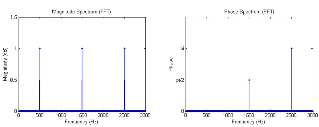
re-spectively and with initial phases 0,π/2 andπrespectively. Adding those three sine waves, the result is a complex vibration (waveform) that is represented in (d). 7 2.4 Magnitude spectrum and phase spectrum of the waveform in Figure 2.3.d,

fre-quency domain representations. 8

2.5 A spectrogram of a music. 9

2.6 Windowing an input signal, from [32]. 9

3.1 MFCC’s feature from 2 music samples, Classical and Metal. 16

3.2 DWCHs of 10 music signals in different genres. The feature representation of different genres are mostly different from each other (from [19]). 19 3.3 DWCHs of 10 blues songs. The feature representation are similar (from [19]). 19

3.4 Beat histogram examples, from [42]. 21

3.5 The Bark Scale (from [13]). 22

3.6 Two firsts steps of the RP extraction for a Classical music. a) A spectrogram representation. b) A spectrogram representation after a Bark Scale applied. 23

3.7 Feature set used. 24

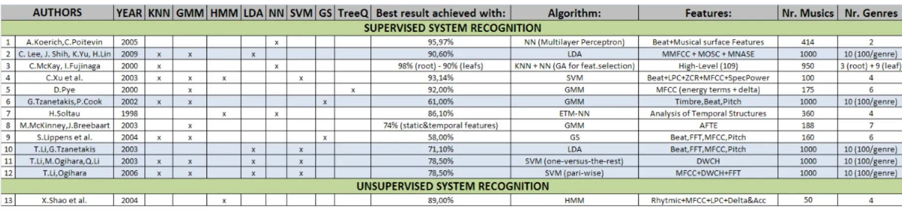
3.8 Summary of previous studies in automatic genre recognition. Each row rep-resents one study and for each one we present: authors, published year, algo-rithms tested, best accuracy result, algorithm used to achieve the best result, features extracted to achieve the best result, number of music samples classified and number of different genres tested. There are twelve studies that used a su-pervised approach while only one study used an unsusu-pervised approach. Blue background is used to specify the studies that used the same database (rows 2,

6, 10-12). 28

4.1 Learning process illustration where rectangles represent data (vectors or matri-ces) while oval boxes are used for transformations/processes. 38 4.2 Similarity matrix from 165 music titles (11 different genres). 40

(12)

(13)

List of Tables

3.1 Parameterization of matrixΣ_c in the Gaussian model and their geometric

inter-pretation. 34

5.1 Best results achieved in "Test A". 55

5.2 Best results achieved in "Test B". 58

5.3 Confusion matrix of classification process using feature set combination nr.1. Number of musics labeled with a specific genre associated to a cluster id (7

clusters). 63

5.6 Accuracy results of a classification process for 3 different feature combinations. 63 5.7 Mahalanobis distance examples calculated from 4 distinct musics based on

fea-ture combination number 2. The first column represent the correct group index, the second corresponds to the attributed group by our system, and next, the Ma-halanobis distances calculated are shown (each distance is from the music to a specific cluster). Distances in bold are those chosen by the system. 64

(14)

(15)

Acronyms

AFTE Auditory Filterbank Temporal Envelopes. 30

ANN Artificial Neural Networks. 26, 30, 31

ASC Audio Signal Classification. 10, 14

BIC Bayesian Information Criterion. 34

DDL Description Definition Language. 2

DWCHs Daubechies Wavelet Coefficient Histograms. 18, 29

EM Expectation Maximization. 26, 33

ETM-NN Explicit Time Modeling with Neural Networks. 30

FFT Fast Fourier Transform. 7, 8

FT Fourier Transform. 7

GHSOM Growing Hierarchical Self-Organizing Map. 31

GMM Gaussian Mixture Models. 25, 29, 30

GS Simple Gaussian. 30

HMM Hidden Markov Model. 26, 31

KNN K-Nearest Neighbor. 25, 30

LDA Linear Discriminant Analysis. 26, 29, 35

LPC Linear Prediction Coefficients. 18, 30, 31

MBCA Model-Based Clustering Analysis. 33–35, 41, 54, 55, 65

(16)

PCA Principal Component Analysis. 31, 32, 36, 40, 42, 45, 65

PDF Probability Density Function. 26

RH Rhythm Histogram. 21, 23

RMS Root Mean Square. 17, 52

RP Rhythm Patterns. 21, 23

SSD Statistical Spectrum Descriptor. 13, 15, 21, 23, 51, 52

STFT Short-Time Fourier Transform. 8, 14, 15, 20, 51, 52

SVM Support Vector Machines. 26, 29, 30

WT Wavelet Transform. 20

XML Extensible Markup Language. 2

(17)

1

. Introduction

1.1 Introduction and Motivation

In this study we explore automatic music genre recognition and classification of digital music. Music has always been a reflection of culture differences and an influence in our society. Today’s digital content development triggered the massive use of digital music. Nowadays, digital music is manually labeled without following a universal taxonomy, thus, the labeling process to audio indexing is prone to errors. A human labeling will always be influenced by culture differences, education, tastes, etc. Nonetheless, this indexing process is primordial to guarantee a correct organization of huge databases that contain thousands of music titles.

These databases are growing everyday and it is now very easy to choose, beyond such offer, to which music, artist or genre we want to listen. Such amount of data needs to be well organized such that the constant updating does not interfere with the ability to generate correct query answers. A correct classification of each music can be the key to maintain a well structured and organized database. Many properties can be used to classify music, although, music genre is, perhaps, the most commonly applied. Often, music can be associated to one or more musical genres. Such genres can be seen as single leafs in an enormous hierarchical tree of genres that is always growing up. Currently, musical genre classification is used in music stores, Internet sites, etc. to organize music in different sections so clients retrieve, without difficulty, their favorite music. In this study, our interest is about music genre organization.

A genre is, by definition, "a style or category of art, music, or literature" [37] or "a class or category of artistic endeavor having a particular form, content, technique, or the like" [1].

Boundaries between multiple musical genres are not easy to describe. A music can be defined using different criteria such as geographic places, history time, instruments used, etc. For in-stance, while a certain music can be labeled as an "Indian Music" in Europe, it will, for sure, not be recognized as "Indian Music" in India.

Although everyone understands music like an universal language, the labeling process is not a simple problem. To solve it, most of the time an artist is associated to one musical genre. This can be a possible solution although, is not a strong one. An artist does not have to follow the same music references in his entire career, even a single album can mix multiple genres. So, which line can we follow to associate a correct music genre with a song? Is there any global music genre taxonomy followed by everyone?

(18)

dia Content Description Interface (MPEG-7) and MPEG-1 Audio Layer 3 (MP3). Those two formats have, between other functionalities, a specific way to deal with extra information rel-ative to multimedia content. Next we will briefly explain why these formats are important in dealing with music, and more precisely, why they gain a significant importance in music genre classification.

MPEG-7 is a standard that has the purpose of describing multimedia content. It supports information interpretations which can be read by many applications by simplified mechanisms. This information enriches multimedia content to automatic systems but also to human users. Metadata information follows a structure defined by a Description Definition Language (DDL). DDL is a schema language to represent the results of modeling audiovisual data (descriptors and description schemes). This structure definition is important to allow different applications to manage multimedia information always following the same protocol. To keep metadata in-formation attached with multimedia content, Extensible Markup Language (XML) is used. This format brought a possibility to manage music information in a new approach. More information about this multimedia standard can be found in [33].

MP3 is a widely used digital audio format. Such popularity is due to its power to compress while maintaining a reasonable audio quality. MP3 reduces drastically the size of music files, which become easy to manage, store and share. We will not deepen MP3 specifications but an important source of information about this encoding algorithm can be found in [12]. There is a particularity in those files that is important to highlight, each one is capable to store extra information about music in different tags calledID3 tags. These tags contain information like

title, artist name, album, year, etc. In newer versions, advanced data can be found, such as music lyric, album art or user comments. Once filled, most commonly used MP3 players are able to present such properties during a reproduction. Generally, ID3 tagsare filled manually

(19)

3

processes results. A wrong decision made by a "tagger" can quickly spread over the network and become hard to correct being often detected human errors in music genre classification. So why don’t we try an automatic labeling process? Can this automation improve reliability in genre classification?

An automatic classification based on good features and using a correct classification algo-rithm may prevent the occurrence of errors related to manual labeling. As a consequence it will raise information reliability, which will benefit music consumers and also industrial com-panies. A perfect automatic classification is hard to achieve but we believe, based on related work results, that it is possible to obtain good results in such task.

Our main goal is to create an audio indexing system which is able to respond to this classifi-cation issue. An unsupervised automatic music genre classificlassifi-cation is intend to be implemented to organize a set of music by their genreonlybased in their audio properties. With an

unsuper-vised approach, new genres can be also classified since we do not restrict the number of genres as a supervised model would do. For that, we propose a learning methodology for automatic genre classification which is able to group several music samples by their music characteristics (learning process). This intends to group the music samples into different clusters only based on audio features and without any previous knowledge on the genre of the samples, and therefore it follows an unsupervised methodology. In addition a Model-Based approach is followed to generate clusters as we do not provide any information about the number of genres in the data set. It would not be plausible to initially give the number of existing genres to our system, this would be the complete opposite of our main goal, which is to identify the number of genres represented in a music data set. Features are related with rhythm analysis, timbre, and melody, among others. As these features represent a large number of dimensions, a redundancy reduc-tion technique is necessary to reduce dimensionality of our extracted data. As a final result, we will have several clusters composed by music samples which present identical audio properties. These groups will be the result of our genre classification, which we can query to know which musics are in a specific cluster or which musics have the same characteristics as our favorite music, for instance.

(20)

aim of our project and present our motivations; Fundamental Concepts (Chapter 2), where

we introduce some sound fundamental concepts in Section 2.1, a discussion about music genre recognition in Section 2.2, more precisely concerning genre taxonomy in Section 2.2.1 and au-tomatic music genre recognition in Section 2.2.2; Methodology and State-of-the-art

(Chap-ter 3), where related work on automatic music genre recognition is discussed as well as different methodologies that will be adopted in our solution. Section 3.1 introduces the main features tested and explains some properties of those features; Section 3.2 presents the main classifica-tion algorithms explored in sound classificaclassifica-tion; accuracy results are presented and discussed in Section 3.3; an introduction to the redundancy reduction approach is discussed in Section 3.4; and finally a discussion concerning the clustering problematic is shown in Section 3.5;My Con-tribution(Chapter 4) will explain how the learning system (Section 4.1) and the classification

system (Section 4.2) are implemented; Results (Chapter 5) presents all the important results

and details about the submitted tests; and finally, Conclusion and Future Work(Chapter 6)

(21)

2

. Fundamental Concepts

This chapter introduces some fundamental aspects that, we believe, are important for music genre recognition. Section 2.1 discusses basic knowledge about digital sound and Section 2.2 introduces the music genre recognition thematic with a reflection about genre taxonomy and the main steps that have to be taken in order to achieve an automatic music genre categorization.

2.1 Sound

We live in an environment where the air has an important role in the propagation of signals. Air molecules tend to move in a random direction. When an object vibrates, it triggers a move-ment to the closest air molecules and forces them to follow the movemove-ment direction creating a wave. This wave is then propagated in a spherical form. Once it arrives near the human ear, the eardrum (tympanic membrane) receives these vibrations which are then transmitted to the ear structures and may result in audible sound. More information about this topic can be found in [46].

Joseph Fourier 1 derived an important theorem which states that any vibration, including sounds, can be resolved into a sum of sinusoidal vibrations, where each sinusoid corresponds to a frequency component of the sound. The sum of sinusoidal vibrations is called Fourier Series. Any sound can thus be represented by different sinusoids.

This section introduces and clarifies important concepts concerning sound analysis that can be helpful to understand the developed work. Complementary explanations of those concepts can be found in [2, 3, 13, 32, 46]. In the next Section 2.1.1 some concepts around digital sound representation are discussed.

2.1.1 Digital Sound Representation

In Figure 2.1 we show a pendulum movement that is tracing a sinusoid, also called sine wave (particular sinusoid with starting phase=0°). This wave repeats infinitely the same movement with identical periods (cycles of oscillation), and can easily be described as a continuous oscil-latory movement characterized by three important aspects: amplitude, frequency and starting

1_{Jean Baptiste Joseph (1768-1830), Baron de Fourier French engineer, mathematician and physicist best known}

for initiating the investigation of Fourier series and their application to problems of heat transfer.

(22)

Figure 2.1: A swinging pendulum drawing a sinusoid (sine wave), from [3].

Figure 2.2: A cycle of a sinusoid, with amplitude, phase and frequency, from [3].

phase (Figure 2.2).

Amplitude is often expressed in decibels (dB) and it refers to the amount of vibration dis-placement. Frequency is the number of cycles that a sinusoid performs per second and is mea-sured in Hertz (Hz). If a sinusoid completes 100 complete cycles in 1 second, then it has a frequency of 100 Hz. Starting phase represents the point in the displacement cycle of a sinusoid in which the sine wave starts. If the wave begins with a positive amplitude, starting phase must be between 0° and 180° (0-π radians). Otherwise starting phase lies between 180° and 360° (π-2πradians). The relationship between amplitude displacement and time can be described by the following equation:

D(t)=Asin(2πf t+θ) (2.1)

where A is the maximum amplitude, f is a frequency measurement, t is a time measure, θ

represents the starting phase and finally D(t) is the correspondent instantaneous amplitude of

(23)

7

Figure 2.3: (a), (b) and (c) represent sinusoids with frequencies 500, 1500 and 2500 Hz re-spectively and with initial phases 0,π/2 andπrespectively. Adding those three sine waves, the result is a complex vibration (waveform) that is represented in (d).

As mentioned above, a vibration consists of a sum of one or more sinusoids. A vibration that is composed by several sinusoids is called acomplex vibration, although, if it consists of

only one sinusoid, it is asimple vibration. Figure 2.3.a-c shows three sinusoids with frequencies

500, 1500 and 2500 Hz respectively. In the bottom graph (Figure 2.3.d), a complex vibration is plotted representing the sum of the sinusoids of 500, 1500 and 2500 Hz. The representation of such sum is calledwaveform.

A mathematical procedure called Fourier Transform (FT), converts a waveform (time do-main) into a spectrum (frequency dodo-main). An efficient implementation of FT that uses discrete-time signals is called Fast Fourier Transform (FFT). With this technique (FFT), themagnitude spectrumandphase spectrumof a specific waveform can be obtained. Those two elements are

(24)

Figure 2.4: Magnitude spectrum and phase spectrum of the waveform in Figure 2.3.d, frequency domain representations.

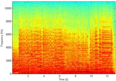
Sound may also be portrayed using another approach entitled spectrogram. While a

spec-trum is a 2D representation (frequency_×magnitude) a spectrogram corresponds to a 3D graphic (time_×frequency_×magnitude). A spectrogram illustrates the magnitude variation along time and frequency. Figure 2.5 shows aspectrogram where higher magnitude values are expressed

in dark colors while light colors are intended for lower amplitude values.

The Short-Time Fourier Transform (STFT) uses FFT to compute the time-varying spectra of the signal. The termshort-time derives from a process calledwindowing processwhere an

input signal is divided into small segments with a specific time duration, usually between 1 ms and 1 second. Figure 2.6 illustrates this process. Since a Hamming function, which is not a rectangular function, is usually chosen to multiply with the signal segment (like illustrated in Figure 2.6), there is a need to overlap those segments to avoid some loss of information. The next step is to extract a magnitude and phase spectrum from each window using the FFT. Thus, STFT gives us a representation of the time-spectral variation of the signal (Figure 2.5).

Three sound representation techniques were presented in this section: waveform, spectrum and spectrogram. Those methods are used in sound analysis each one with a different purpose. For instance, a spectrogram is better if we want to find a specific sound (instrument, voice, etc.) in the middle of a music, while waveforms are useful when looking for a weak reflection following a short sound, and a spectrum representation can be useful to observe the sound’s

(25)

9

Figure 2.5: A spectrogram of a music.

(26)

music taxonomies on the Internet [29]. They analyzed the classification methods of three dif-ferent sources, which are all well known Internet music retailers (Amazon2_{, AllMusicGuide}3 and MP3 web site4_{) and looked for similar structures between them. Those three taxonomies} presented huge differences concerning the treatment of relevant information like genealogical hierarchies, geographical information, historical period, etc. and also how they are prepared to receive a new genre. It was easily concluded that the skeletons were extremely different and their combination would be an hard task. Yet, those taxonomies work perfectly when used by a client that is searching for a specific music, the aim is accomplished with more or less effort.

An inconsistency appears when the data is exploited by software (for instance, search mech-anism). To solve this problem, F.Pachet and D.Cazaly suggested a new method to create a genre taxonomy following some basic criteria. They reduced considerably the number of different genres applying a stronger connection between each one and introduced new descriptors (like danceability, audience location, etc.). It is clear that a world taxonomy is hard to implement but this solution can be a good starting point to develop an universal music genre classification.

2.2.2 Automatic Music Genre Recognition

Audio Signal Classification (ASC) is a research field that explores different areas such as speech recognition, music transcription and recently speech/music discrimination. The aim of ASC is to label an audio signal based on its audio features, i.e., with a computational analysis of audio properties, to be able to identify to which class the analyzed signal belongs. Two main steps are needed during this process: feature extraction and classification. As part of ASC,

(27)

11

music genre recognition also needs to follow these two steps.

2.2.2.1 Feature Extraction

Feature extraction is the first step in music genre recognition. This process is very important: automatic genre recognition can only be successful if music samples from different genres are separated in the space formed by the extracted features. When a set of music begins to be analyzed, a lot of values are extracted from each single music, and from that point, these values can be seen as the music files "lawyers". These values will represent each music during all the genre recognition process and, from now one, all complementary information that we could access, from a MP3 file or MPEG-7 file, will not be used. The importance of this process is to guarantee that the values extracted will be enough to distinguish different music genres and emphasize boundaries between different music styles.

A feature is, by definition, "a distinctive attribute or aspect" [37]. To better understand what a feature is, we propose a simple exercise. Imagine that we want to know the average height of a class. To obtain it, we will imperatively need to know the height of each student. Once we have this information, we are able to use it for different purposes such as, average height, maximum, minimum, etc. In this simple example, the feature used is human body height.

Features from audio signals can be related to dimensions of music as melody, harmony, rhythm, timbre, etc. Two main feature groups can be set: computational features and perceptual features. Those groups are exploited in Section 3.1 where most commonly used musical features are described as well as articles in which those feature sets have been tested.

2.2.2.2 Classification

Once the features are extracted, the classification process is the next step. Basically, this step will use the extracted values to define boundaries between different genres, and afterwards it associates each music to one (or more) genre. Three distinct paradigms can be followed at this stage, each one with their own properties: expert systems, unsupervised learning or supervised learning. Before a decision about which paradigm is the right one do adopt, we need to study their differences. The goal can be hit with any of these paradigms, but some are more useful to solve our problem. Let us find out why.

(28)

Supervised learning is the most used paradigm to classify music samples according to their genre. Manually labeled data is required to train the system in a first stage. During this training stage, relationships between features values and genres will be created. After this period, the system is able to classify new unlabeled data based on the previous training. This paradigm differs from the expert system paradigm since it does not need a complete genre taxonomy, it only requires labeled data that will be used to automatically create the relationships between the features and the categories. This technique is explored in [16–20, 22, 25–27, 30, 38, 42, 45].

(29)

3

. Methodology and State-of-the-art

In this chapter we present all the details concerning features extraction and the classification process used in our implementation. Here we also present the state-of-the-art concerning auto-matic music genre recognition and discuss about other features and algorithms used in this area. As mentioned in Section 2.2.2, two main steps are needed in automatic genre recognition: fea-ture extraction, which is discussed in Section 3.1, and classification, described in Section 3.2. In Section 3.3, results from several studies are compared based on features and classification used.

3.1 Feature Extraction for Automatic Music Genre Recognition

Feature extraction is the first process to be executed in automatic music genre recognition. Next we describe all the features we have explored as well as some commonly known features that are used in music genre recognition. We grouped the features into three distinct groups: computational features, perceptual features and high-level features. We considered as com-putational features (Section 3.1.1) the ones that does not present any musical meaning, they only describe a mathematical analysis over a signal. In the opposite, perceptual features (Sec-tion 3.1.2) represent, in some way, the percep(Sec-tion that a human has listening to a music. Finally, we also focus some features named as high-level features (Section 3.1.3) which are able to represent a music event using a different perspective.

Before a more detailed description of each feature, it is important to note that some of these feature sets have a very high dimensionality and it is more efficient to describe them with less dimensions, always ensuring their "meaning". For this purpose, we use Statistical Spectrum Descriptor (SSD) which consist in seven statistical descriptors: mean, median, variance, skew-ness, kurtosis, min- and max-value [21]. Using these mathematical values, T.Lidy and A.Rauber presented interesting results. With this representation, we drastically reduce the number of di-mensions to seven ensuring that the main statistical properties of the analyzed feature set are maintained. Whenever this property is calculated, we clarify over which set these statistics are processed. These properties can limit the description of the analyzed features since they assume a perfect Gaussian data representation although we choose to use these descriptors since they already present interesting results.

(30)

tral Flux, Zero-Crossing Rate (ZCR), Low Energy and Mel-Frequency Cepstral coefficients (MFCCs). The spectral properties can follow two different approaches, calculate values over each window of a STFT (obtain a set of spectral values for each window) or they can be cal-culated directly over an audio spectrum (and we only have one value for that music). Usually, these values are calculated after a STFT. As long as we obtain a set of values with a significant dimension, means and variances are calculated and used as another feature value. This two ad-ditional properties represent the "behavior" of these spectral values. How do we calculate these properties? Let us look in detail to each feature:

Spectral Centroid represents the "center of gravity" of the magnitude spectrum. Next we

present how the centroid is calculated:

Ct=

PN

n=1Mt[n]∗n

PN

n=1Mt[n]

whereMt[n] is the magnitude at frametand frequency binn.

Spectral Rolloff corresponds to the frequency Rt which concentrates 85% of the magnitude

distribution below it.

Rt X

n=1

Mt[n]= N

X

n=1

Mt[n]∗0.85

Spectral Flux corresponds to the square difference between the normalized amplitudes of suc-cessive spectral distributions.

Ft= N

X

n=1

(31)

15

where Nt[n] and Nt−1[n] are the normalized magnitude of the Fourier transform at the current framet, and the previous framet₋1, respectively.

ZCR represents the number of times the audio waveform crosses the zero axis per time unit:

Zt=

1 2

N

X

n=1

|sign(x[n])₋sign(x[n₋1])_|

where thesignfunction is 1 for positive arguments and 0 for negative arguments andx[n]

denotes the time domain signal for framet.

Low Energy is the percentage of frames that have lower energy than the average energy over

the whole signal. It measures the amplitude distribution of the signal and can be a good feature to distinguish between music genres. As an example, a music which presents long silence periods will have a larger low-energy once compared to a music with few silence periods. This feature is based on the analysis over the spectrogram of a sound.

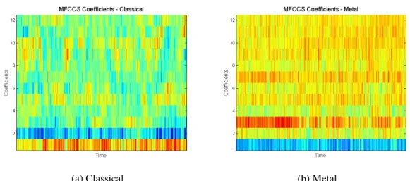
MFCCs are one of the most popular set of features used in pattern recognition, particularly in

speech recognition. Based on the auditive human system model, it uses a Mel-frequency scale to group the FFT bins. After a STFT transformation the log-based magnitude is filtered by a triangular filter bank that is constructed based on 13 linearly-spaced filters (133.33Hz between center frequencies). A 10 log base is calculated and a cosine trans-formation is applied to reduce dimensionality.

Although this feature set is based on human perception analysis, we classify it as a com-putational feature since it may not be understood as human perception of rhythm, pitch, etc. It would be acceptable to classify the MFCCs as perceptual as they try to simulate the human auditory perception based on the Mel scale.

(32)

(a) Classical (b) Metal

Figure 3.1: MFCC’s feature from 2 music samples, Classical and Metal.

As mentioned above, these presented features were combined in a set calledtimbral texture featuresin some previous works [16, 20, 22, 42]. This set is used in many studies related with

automatic music genre classification.

G.Tzanetakis and P.Cook were the firsts to extract these features from several music files [42]. Later, T.Li and G.Tzanetakis presented a refinement of this article achieving, with the same features but different classification algorithms, better accuracy results [20]. S.Lippens et al. compared accuracies between human and automatic music genre classification also with tim-bral texture features [22] and they conclude that the use of features derived from an auditory model have similar performance with features based on MFCCs.

A. Koerich et al. also include these features in their study [16]. A particular difference exists in their approach concerning the extraction of features. Features are not extracted from the whole music file or from a single part of the music, they are extracted from three different sections of the music file: begin, middle and end. A. Koerich’s team believes that this small detail could make a difference when a music does not behave well in time, i.e., the amplitude variation can be very high.

(33)

17

T.Li and al. also exploit timbral features in their researches [18, 20].

Apart from the timbral texture features, there are also other useful computational features:

Root Mean Square (RMS) is an approximation of the volume/loudness value:

pn=

v u t

1

N

N−1 X

i=0

s2n(i)

where N is the frame length,sn(i) denotes the amplitude of the ith sample in the nth frame.

Bandwidth is a energy-weighted standard deviation and it measures the frequency range of the

signal [11, 23]:

Bt=

v t PN

n=1(Ct−log2(n))2.Mt[n]

PN

n=1Mt[n]

Bt is the bandwidth of framet, withCtas the centroid andnas a frequency bin.

Uniformity measures the similarity of the energy levels in the frequency bands [11, 23]:

Ut=− N

X

n=1

Mt[n]

PN

n=1Mt[n]

.logN

Mt[n]

PN

n=1Mt[n]

Ut is the uniformity of framet.

While the features described so far were all explored in this work, there are many more features that are not used by our classifier. Below we present some of those features that can lead to good results in Music Information Retrieval (MIR).

C.Lee et al. extracted MFCCs features combined with two other feature sets [17]:

Octave-Based Spectral Contrast (OSC) represents the spectral properties of a music signal.

A spectral contrast can be defined over a spectral analysis, in which peaks and valleys represent harmonic and non-harmonic components of the music respectively.

Normalized Audio Spectral Envelope (NASE) represents the power spectrum of each audio

(34)

extracted for vocal music analysis.

Daubechies Wavelet Coefficient Histograms (DWCHs) was proposed by T.Li et al. and is

discussed here since it presents good results in automatic genre classification [18, 19]. In summary, this feature set extraction presents the following steps:

1. Wavelet decomposition of the music signal;

2. Construction of a histogram of each subband;

3. Computation of the first three moments of all histograms;

4. Computation of the subband energy for each subband;

To illustrate the advantages of this feature set, Figure 3.2 shows DWCHs from ten diff er-ent music genres. In this figure we can see DWCHs features of ten music genres based in G.Tzanetakis and P.Cook database with Blue, Classical, Country, Disco, Hip hop, Jazz, Metal, Pop, Reggae and Rock music [3]. Analyzing the different graphics, we can see that for each music type we have a different representation. For instance, Blues songs show a very different DWCHs graphic from Pop or Rock. If DWCHs are capable to present distinct values for each music genre, they can be very useful in automatic categorization of music.

(35)

19

Figure 3.2: DWCHs of 10 music signals in different genres. The feature representation of different genres are mostly different from each other (from [19]).

(36)

Rhythmic Content (Beat)

The rhythmic content of a music can be important in genre recognition. Rhythm has not a precise definition but it can be seen as a temporal description of music, i.e., it contains informa-tion such as: the beat, the tempo, the regularity of the rhythm and time signature. This feature set is obtained from the beat histogram analysis, which allows to explore the periodicities of the signal.

The beat histogram is obtained by decomposition of a music signal using Wavelet Transform (WT), an alternative technique to the STFT. From this decomposition, the envelopes of each band are summed and the autocorrelation of the resulting function is calculated. Analyzing the autocorrelation function, the peaks are accumulated into a beat histogram.

From this beat histogram, the usually meaningful information extracted is:

1. Relative amplitude (divided by the sum of amplitudes) of the first and second histogram peak;

2. Ratio of the amplitude of the second peak divided by the amplitude of the first peak;

3. Periods of the first and second peak;

4. Overall sum of histogram;

A repetitive music will present strong beat spectrum peaks at the repetition times revealing both tempo and relative strength of particular beats. Thus it can be used to distinguish between two different kinds of rhythms at the same tempo.

(37)

21

Figure 3.4: Beat histogram examples, from [42].

music genres are presented where is perceptible the differences between each histogram. Other studies also used this feature set [16, 18, 19, 22, 45].

Rhythm Patterns

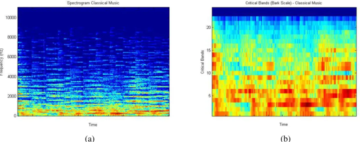
Rhythm Patterns (RP) are not a complete description of rhythm neither a total pitch de-scriber [21]. This feature represents the loudness sensation for several frequency bands in a time-invariant frequency representation. To obtain RP of one music some psycho-acoustic pro-cessing steps are required, and once all transformations are completed, two distinct features can be calculated: SSD and Rhythm Histogram (RH). First, let us start with the RP extraction process. Below we explain the main steps required to obtain this feature.

1. A Short-Time Fourier Transformation is applied to the signal representation. A spectro-gram is obtained (Figure 3.6a); (as default values, 512 samples windows are used with a Hanning window function of 23ms and 50% overlap)

2. A Bark scale1 _{is applied. The spectrogram is grouped using 24 critical bands. More} details in [47] (Figure 3.6b);

1_{Bark scale is an absolute frequency scale which is a measure of critical-band number. In table 3.5 the Bark}

(38)

3. Transform the last spectrogram into a decibel scale (dB).

4. Compute loudness levels through equal-loudness coutours (Phon).

5. For each critical band, calculate the specific loudness sensation (Sone).

6. At this step, a new Fast Fourier Transform is applied to the Sone representation. This new transformation presents a time-invariant representation of the 24 critical bands which shows an amplitude modulation with respect to modulation frequencies that can be seen as a rhythmic descriptor. As humans are not able to perceive rhythm beyond a range from 0 to 43Hz, the considered amplitude modulation is between 0 and 10Hz.

7. Weight modulation according to human hearing sensation and emphasizing distinctive beats from the previous results.

As earlier mentioned, psycho-acoustic phenomena are incorporated in this analysis. In steps 2 to 5 and 7 some studied techniques involving human hearing system are incorporated to in-crease accuracy results.

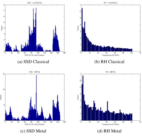
Once RP obtained, some properties can be computed as describers of those values.

After step 6 a SSD (Figure 3.7a and Figure 3.7c) feature set is calculated which is able to describe the audio content according to the occurrence of beats or other rhythmic variation of energy. For each one of the 24 bands, 7 statistical moments are calculated: mean, median, variance, skewness, kurtosis, min- and max-value. The resulting feature set is a vector with 168 dimensions.

(39)

23

(a) (b)

Figure 3.6: Two firsts steps of the RP extraction for a Classical music. a) A spectrogram representation. b) A spectrogram representation after a Bark Scale applied.

are summed up to reach a histogram of "rhythmic energy" per modulation frequency. This histogram will present 60 dimensions which reflect frequency range between 0 and 10Hz.

Pitch Content (Melody, Harmony)

Pitch content features are used to describe melody and harmony of a music signal. The extraction method can be simply explained and is based on various pitch detection techniques. The main goal is to obtain a pitch histogram from where pitch content can be extracted.

Pitch histograms are obtained following four main steps:

1. Decompose the signal (FFT);

2. Obtain envelopes for each frequency band and sum them;

3. From that sum, obtain dominant peaks of the autocorrelation function;

4. Accumulate dominant peaks into pitch histograms;

(40)

(c) SSD Metal (d) RH Metal

Figure 3.7: Feature set used.

G.Tzanetakis et al. demonstrated how relevant the pitch content feature may be in genre classification [43]. G.Tzanetakis and P.Cook also used this feature set [42] following a multip-itch detection algorithm described by Tolonen and Karjalainen [40]. Later, T.Li and G.Tzanetakis refined this work using the same features but with another classification method [20]. As men-tioned before, some other papers related with automatic genre classification followed features proposed by G.Tzanetakis and P.Cook being pitch content analyzed too in [16, 18, 19, 22].

This feature set is widely tested in automatic music genre classification and good accuracy results are achieved when it is used. Music melody is an important property for labeling a music by its musical genre therefore pitch content is often extracted.

3.1.3 High-Level Features

(41)

25

it is stored. Symbolic data, or "high-level" representation, stores musical events and parame-ters while audio data, or "low-level" representation, encodes analog waves as digital samples. Description features can be extracted from both types of representations.

C.McKay brought a different approach to genre classification [25,26]. He defined two types of features, low-level featuresand high-levelfeatures that are extracted from these

representa-tions. Low-level features are based in signal-processing with no explicit musical meaning, e.g., ZCR, RMS, etc. while high-level features are characterized by having a musical meaning, based on musical abstraction, e.g., tempo, meter, etc. Both features can be extracted from low-level data. Still, a better accuracy is hit with high-level features when high-level data is used.

C.McKay tests high-level features using MIDI format, which is a high-level data representa-tion. C.McKay explains the main advantages and disadvantages of using the MIDI format [26]. Some features commonly used in genre classification are unavailable in such format which could reduce the average accuracy classification, although, since symbolic data was an unex-ploited area concerning musical genre classification, C.McKay developed an application based on high-level features that could bring a new focus into symbolic data representation. Some important musical knowledge such as, precise note timing, voice and pitch are available which opens a door to exploit those new features. At the end, this experience revealed that some losses of usual information, as timbral content, could not be as significant as it may seem.

3.2 Classification Algorithms for Automatic Music Genre Recognition

After the feature extraction phase, we have now data that can be analyzed in the classifica-tion process. Two different approaches can be adopted in music genre recognition: supervised recognition and unsupervised recognition (see Section 2.2.2 for more details). Below, we de-scribe the most commonly used algorithms in automatic music genre recognition. As we will be able to see in this section, most of these algorithms follow a supervised approach.

K-Nearest Neighbor (KNN) is one of the most popular algorithms in instance-based learning.

(42)

several studies [17–19, 22, 30, 42, 45]

Hidden Markov Model (HMM) is widely used in speech recognition due to its capacity to

handle time series data. It is a double embedded stochastic process that handles two distinct processes: one process is hidden and can only be observed over another stochastic process (observable) which produces the time set of observations. This method can be defined by its number of states, the transition probabilities between its states, the initial state distribution and the observation symbol probability distribution. It can be used in supervised systems [34, 38] but also in unsupervised systems [35].

Linear Discriminant Analysis (LDA) aims to find the linear transformation that best

discrim-inates among classes. The classification is performed in the transformed space using some metric (e.g. Euclidean distances). This classification algorithm presents one of the best accuracy results known and it was used in several different articles [17–20]. An extensive explanation of this algorithm can be found in [10].

Support Vector Machines (SVM) is a very popular binary classification method applied in

pattern recognition [44]. This algorithm intends to find a hyper plane that separates neg-ative points from positive ones with a maximum margin. Initially designed for binary classification, it can also be used to a multi-class classification applying different ap-proaches such as pair-wise comparison, multi-class objective functions or one-versus the rest. This algorithm is explored in [18–20, 45].

Artificial Neural Networks (ANN) are composed by a large number of highly interconnected

(43)

27

Below, in Section 3.3, results from different studies are presented. Different combinations between features and classification algorithms are discussed.

3.3 Databases

&

Results

3.3.1 Supervised System Recognition

(44)

(45)

29

Five distinct studies used the same database which contains ten musical genres (Blues, Clas-sical, Country, Disco, Hip hop, Jazz, Metal, Pop, Reggae, and Rock) with one hundred excerpts of music for each genre (rows 2, 6, 10-12). These excerpts of the data set were taken from radio, compact disk, and MP3 compressed audio files. They were stored as 22 050 Hz, 16-bit, mono audio files. An important effort was made to ensure that the musical sets truly represent the corresponding musical genre [17–20, 42].

In 2002, G.Tzanetakis and P.Cook created this database to exploit musical genre classifica-tion of audio signals [42]. They achieved an accuracy of 61% combining timbre, beat and pitch feature sets with a GMM classification algorithm. In 2003, T.Li and G.Tzanetakis, realized new tests to this database with other classification methods [20]. They achieve a correct classifi-cation result in 71,1% of the tested music using the LDA classificlassifi-cation algorithm applied to a feature set composed by beat, FFT, MFCCs and pitch content.

Also in 2003, T.Li et al. achieved an accuracy of 78,5% using DWCHs to classify music with an SVM algorithm (one-versus-the-rest) [19]. In a later work, T.Li and Ogihara presented more details and shown that DWCHs can achieve good classification results when combined with FFT and MFCCs feature sets [18]. They also obtained a classification accuracy of 78,5% although, it is reached with a pair-wise SVM algorithm. The information in these two articles is contradictory. The presented results are exactly the same, not only the best accuracy, but the confusion matrix is the same using different features and a different classification algorithm. In the first article [19], we believe that some information is missing since the later article [18] presents a different combination (SVM + DWCHs,MFCCs,FFT) that is more plausible (with the same results).

In 2009, C.Lee et al. achieved really good results with the same database on long-term modulation spectral analysis of spectral (OSC and NASE) and cepstral (MFCCs) features [17]. Their best accuracy is 90,6% achieved using LDA classification algorithm.

These five studies apply several combinations of features and classification algorithms to obtain the better accuracy possible. It is clear that the results have improved along the years and now an accuracy rate of 90,6% has been achieved. Although, other studies with better performances are reported in the past years, a direct comparison should not be made since those studies tested different databases.

(46)

C.Xu et al. employ a data set with 100 music samples collected from music CDs and the Internet [45]. This data set contains music from different genres as Classic, Jazz, Pop and Rock. Only 15 titles from each genre were used as training samples. An accuracy of 93% was achieved combining several feature sets (beat spectrum, LPC, ZCR, spectrum power and MFCCs) classified with a SVM.

D.Pye’s database contains 175 samples representing 6 different musical genres, Blues, easy listening, Classical, Opera, Dance and Indie Rock [30]. Musics were split evenly between the training and test sets. By extracting an MFCCs feature set and classifying with a GMM algorithm, D.Pye achieved an accuracy of 92%.

H.Soltau et al. had a database composed by 3 hours of audio data for four categories: Rock, Pop, Techno and Classic [38]. They achieved a recognition rate of 86,1% using their Ex-plicit Time Modeling with Neural Networks (ETM-NN) approach that combines discriminative power of neural networks with a direct modeling of temporal structures.

M.McKinney and J.Breebaart classified 7 different musical genres (Jazz, Folk, Electronica, R&B, Rock, Reggae and Vocal) with a total of 188 samples [27]. An accuracy rate of 74% was achieved using Auditory Filterbank Temporal Envelopes (AFTE), classified by a GMM algorithm.

(47)

31

3.3.2 Unsupervised System Recognition

X.Shao et al. presented a study using unsupervised classification for music genre recog-nition [35]. They achieved an accuracy rate of 89% with a 50 music database that represents 4 distinct musical genres (Pop, Country, Jazz and Classic). Rhythmic content, MFCCs, LPC and delta and acceleration (improvements in feature extraction) were applied to a classification performed by a HMM. However, a quite detailed confusion matrix is presented with a perfect accuracy results in Classical music recognition (100%). The worst results are achieved with the Jazz recognition process, only reaching 76% success. Jazz samples were assumed as Pop music 20% of times. The presented accuracy results allow us to conclude that this unsupervised approach can benefit automatic genre classification since there is no need to previously label a data set to obtain good results in music genre recognition.

A.Rauber et al. applied a Growing Hierarchical Self-Organizing Map (GHSOM) (which is a popular unsupervised ANN) to classify psycho-acoustic features (loudness and rhythm) ob-taining a hierarchical structuring music tree [31]. They tested their implementation with two distinct music databases, one with 77 samples and another with 359. They presented no con-fusion matrix or accuracy results although, an analysis of each created cluster is made looking at the grouped samples. Their results are encouraging despite the few features extracted. It is noticeable that music samples belonging to the same cluster present similar rhythms and "sound styles" for human perception. It is also interesting to notice that music from a single band can fall into several clusters, which reveals a plurality of music genres within a music band. Un-fortunately, no confusion matrix has been presented turning a comparison with other discussed studies impossible, that is why this paper is not included in Figure 3.8.

3.4 Redundancy Reduction

Principal Component Analysis (PCA) is one of the most popular techniques used to reduce the dimensionality of a data set. In this section, our goal is to provide a simple explanation of this technique and discuss some details that we consider important to understand why we use this algorithm. A detailed study about this statistical tool can be found in [24, 39].

(48)

attributes or axis of the initial space). These axis are the uncorrelated final attributes which are presented in a matrix, ordered by descending variances of their values, from the matrix leftmost to the rightmost columns [15]. Since global information is mostly concentrated on the leftmost columns of that matrix, usually, only the first few columns are used to describe the initial data.

3.5 Clustering Problematic

A clustering or grouping process can follow several ways pursuing one common goal: create clusters based on a data set. We will approach two different solutions for such problematic in this section: Partitioning grouping (Section 3.5.1) and Model-Based grouping (Section 3.5.2).

3.5.1 Partitioning Group

In this family we can highlight two commonly known algorithms: k-meansandk-medoids

(details in [14]). Once applied to a data set, they both return as resultk clusters. This number

(k) has to be given by the user.

Ink-means, a cluster is represented by the centroid of its elements. The algorithm attempts

to find a cluster combination such that it maximizes the similarity between each element (music, document, etc.) and the centroid of its belonging group. In the other hand, ink-medoidsa cluster

is represented by one element chosen by the algorithm. Essentially, these two algorithms differ in such a way that whilek-meansgives an equal weight to each element of a cluster to get the

centroid,k-medoidstends to ignore the outliers from a cluster.

Another peculiarity concerning these algorithms is the use of theEuclideanor Manhattan

(49)

33

covariances have an important role in the cluster creation which implies the uniform volume to all clusters. Nonetheless, clusters do not always present a hyper-spherical volume, as it can be seen in [7].

Since, the number of clusters must be set a priori by the user and clusters can present non-spherical volumes, we do not use this approach in our solution. As it will be seen later (Sec-tion 3.5.2) in order to allow non-spherical volumes, we opted for a different kind of distance measure in our solution, and we also do not set the number of clusters a priori to let the al-gorithm find the most appropriate number of clusters. As already mentioned in Chapter 1 our goal is to find the number of clusters of a music data set without any initial information besides the music samples. With a partitioning group model, we would be forced to initially define the number of groups that we wanted to create. However, we would like that this information (number of groups) would be automatically given by our implementation.

3.5.2 Model-Based Group

The Model-Based approach aims to answer two distinct questions:

• Which is the more accurate configuration for each cluster?

• How many clusters must be created?

Just like in the partitioning approach, the model-based approach aims to create clusters based on an initial data set, although, it does not know the number of clusters, nor their shape or orientation in a restrict dimension space.

Based on this model, C.Fraley and A.E.Raftery [7] developed a Model-Based Clustering Analysis (MBCA) in which they represent the data by several models. Each model is composed by some clusters and presents different geometric properties from the other models. As we will see in more detail later, a configurationmodel-number_of_clustersmore plausible is suggested

for each initial data set.

Groups are merged combining the EM algorithm to use a maximum-likelihood criterion and a hierarchical clustering algorithm (see [7] for details). This methodology is based on multivariate normal distributions (Gausians). Thus, the density function has the form:

fc(xi|µc,Σc)=

e(−12(xi−µc)TΣ−c1(xi−µc)) (2π)p2_|Σ_c_|12

(50)

wherexiis an object that belongs to groupcwhich is centered inµc. Each group has an ellipsoid

volume. Covariance matrixΣ_cis responsible for the geometric property of each group, which is why different models result from different parameterizations of its eigenvalues decomposition:

Σ_c=λcDcAcDTc, (3.2)

whereDc is the orthogonal matrix of eigenvectors which determine the orientation of the axis;

Ac is a diagonal matrix whose elements are proportional to the eigenvalues of Σc, and which

determine the shape of the ellipsoid; and the volume is defined by the scalarλc. That way, shape,

orientation and volume of clusters can be allowed to vary between them, or be constrained to be the same for all groups.

In Table 3.1 we can find several models explored by the MBCA algorithm. By analyzing this table we can see that one of the considered strategy matches with thek-meansspecification,

usingEuclideanorManhattandistances which generate hyper-spherical clusters with the same

volume for all clusters (Σc=λI); theΣc=λcImodel, groups are hyper-spherical although their

volume can be variable; with theΣc=λDADT, all groups have an ellipsoidal volume and present

the same shape and orientation; theΣ_c=λcDcAcDTc model is the least restrictive model in which

shape, volume and orientation can differ in all groups; withΣ_c=λDcADTc, only the orientation

can change between groups; lastly, whenΣ_c=λcDcADTc all groups present the same shape;

Once all models are created, there is a need to compare them and choose which one is the most accurate. MBCA provides a Bayesian Information Criterion (BIC), that is a measure to compare each pair (model-nr_of_clusters) using Bayes factor. A simply comparison is made

(51)

35

the most reliable model will be chosen and consequently, the number of clusters is defined based on such choice.

As a multi-oriented technique, this approach can be used in several areas. Some interesting results can be seen in [4, 5] concerning document clustering. This algorithm fits perfectly our solution. With MBCA we will be able to, after a feature extraction process, attribute a correct cluster to each music from the data set without any a priori information on the number of clusters. Therefore, MBCA will provide us a finite number of clusters and will tell us which music belongs to each cluster (that is exactly what we were looking for!).

3.6 Conclusion

In this chapter we presented the most relevant and commonly used features in music genre recognition as well as the most studied classification algorithms used for the same purpose. As mentioned above, supervised recognition has much more documentation related to genre classification than unsupervised recognition.

In supervised systems, the high number of studies published until now demonstrates a clearly improvement in accuracy results along the past years. Once again, it is important to understand that results achieved from one study can only be compared with another one if both use the same music database. As mentioned before, five studies based their implementation in the same database, and from those studies, the best accuracy achieved was 90,6% extracting MFCCs, OSC and NASE features [17]. A spectral modulation analysis of each feature set was applied and classification was performed by a LDA algorithm. This accuracy was achieved in a 1000 music database representing 10 different genres.

(52)

(53)

4

. My Contribution

Now that all the important concepts concerning our problem were introduced, this chapter will present a detailed explanation of the proposed solution. There are two main goals on this implementation: on the one hand, we want to cluster music samples (from the training data) according to their genre, and, on the other hand, we want to be able to classify new (test) music samples. Clustering music is a learning process which is able to organize them according to their audio features. Once the clustering is done, the classification of new test samples is done according to the clusters learned during the learning phase. This chapter is organized in two sections: one that explores how clustering of the training samples is done (Section 4.1) and another that discussed the classification of the test samples (Section 4.2).

4.1 Learning Process

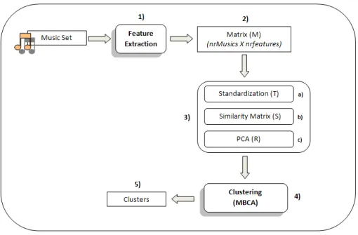
The learning process aims to organize several music samples into clusters without any initial information besides the feature set values of these samples. Let us try to clarify the reader about which steps are needed in the learning process. Figure 4.1 plots the system organization where different transformation steps and data representation can be clearly identified. To easily understand how it works, we will follow the sequence shown in the referred figure and explain it step-by-step. We use rectangles for input/output values while ovals represent computation processes.

1) The system extracts several features (previously selected) from the music samples in the data

set;

2) As a result of step 1 we have a data set matrix (M) in which each line characterizes one

music sample while columns represent a specific feature;

M=                     

m1,1 m1,2 · · · m1,F

m2,1 m2,2 · · · m2,F

..

. ... . .. ... mN,1 mN,2 · · · mN,F

                     ,

wheremm,f is the value of the fth feature for music samplem.

(54)

Figure 4.1: Learning process illustration where rectangles represent data (vectors or matrices) while oval boxes are used for transformations/processes.

3) Once our data set matrix is obtained, some transformations need to be performed.

(a) Standardization - This process aims to scale each feature (that is, each column of the data set matrixM) such that the features have equal variances (i.e., importance).

For this purpose, it creates a new matrixT that has the same dimension as matrix M. T=                     

t1,1 t1,2 · · · t1,F

t2,1 t2,2 · · · t2,F

..

. ... . .. ... tN,1 tN,2 · · · tN,F

                    

wheretm,f stands for the value of the standardized value of music mfor feature f.

To calculate each new cell ofTwe apply the equation below:

tm,f =

mm,f−mean(m.,f)

p

var(m.,f)

(55)

39

wherem.,f is the fth column of matrixM. Variance is obtained from:

var(m.,f)=

1

N

X

i=1

(mi,f−mean(m.,f))2, (4.2)

and the mean from

mean(m.,f)=

1

N

X

i=1

mi,f, (4.3)

whereN is the number of music samples.

(b) Correlation Matrix - At this step, matrixS(the similarity matrix) is calculated from

matrixT. Spresents different dimensions fromT. Since it is a correlation matrix, Sis a symmetric matrix, where the number of lines and columns is the number of

music samples in the data set. Each cell of this matrix represents the similarity between two music samples. With such similarity matrix, it is expected that music titles which belongs to the same genre present, higher correlation values between them. Based on theTmatrix we next present the calculation of the similarity for a

generic cell of this matrix:

si,j=

cov(i, j) √

cov(i,i)_∗ pcov(j,j), (4.4)

whereiand jrefer to music samples. Scan be seen as:

S=                     

s1,1 s1,2 · · · s1,N

s2,1 s2,2 · · · s2,N

..

. ... . .. ... sN,1 sN,2 · · · sN,N

                    

The covariance between samples,cov(i,j), is obtained based on the equation:

cov(i,j)= 1

F₋1

F

X

f=1

[ti,f−ti,.]∗[tj,f−tj,.], (4.5)

whereFis the number of features used (that is, the number of columns inMandT)

(56)

Figure 4.2: Similarity matrix from 165 music titles (11 different genres).

Figure 4.2 plots an image of correlation matrixS for 165 music samples (from 11

different genres). The symmetry of the matrix can easily been confirmed in the figure. The color spectrum in the figure goes from dark blue (for lower values) to red (for higher values) and brown (for the highest value, which is 1): the diagonal (brown) has the maximum correlation value (1).

This similarity matrix can be seen as representing a set of music samples by a spe-cial set of attributes: where each attribute characterizes the similarity of the music sample to another music sample in the data set.

(c) PCA - Now that our similarity matrix is calculated, it is important to built a matrix where objects are characterized by a reduced number of final attributes, so it can be submitted to a classification algorithm. Since the number of samples in the data set is usually high, the similarity matrixS usually has a high number of features

(i.e., attributes). Therefore, there is a need to reduce the number of features (that is the dimensionality of the data). In the example given in Figure 4.2, there are 165 attributes, which are too many attributes to characterize the same number of objects. A technique based on PCA will be used to reduce dimensionality.

MatrixSmay be seen as a representation of several music samples characterized by