Orientador: Doutor Pedro Viana Baptista, Professor Associado com Agregação, FCTUNL Co-orientador: Doutor João Carlos Lima, Professor Associado, FCTUNL

i

João Pedro Maurício Rosa

Licenciado

Nanobiophotonics for biomolecular

diagnostics

Dissertação para obtenção do Grau de Doutor em Biotecnologia

Orientador: Doutor Pedro Viana Baptista,

Professor Associado com Agregação, FCT/UNL

Co-orientador: Doutor João Carlos Lima,

Professor Associado, FCT/UNL

iii Copyright em nome de João Pedro Maurício Rosa, e da FCT/UNL.

v A meus pais

vii

ACKNOWLEDGMENTS

The work here presented would not be possible without the support of so many people and institutions that I fear I will forget someone. All the expression of gratitude may not be enough to show the full extent of my thankfulness for all the support throughout the good and bad moments of this journey. However, my most special thanks must be addressed to:

- My PhD advisors, Professors Pedro Baptista and João Carlos Lima, for supporting and putting up with me, for their guidance, advisory and the academic and scientific growth they promoted in me during these years. Thank you for the opportunity of joining the great adventure that was this crazy project. I thank you both for the support, discussions, criticism and dedication to the cause. Most of all, Thank you for believing in me.

I would like to thank Pedro for the constant support and insightful discussions that far exceeded science. Without your pragmatism and vision none of this would have been possible. It is commonly said that “you are who you spend more time with” and I must thank you for who I am now. You have been an example and a beacon in many things. You pushed me and demanded the best of me. You’ve placed your trust in me and I can only hope not to have let you down. Thank you.

I would like to thank João Carlos for the enthusiastic discussions in science and the lessons in life. For allowing me to grow on my terms and for fuelling the dreams that were essential for this project. I will not forget the opportunities you provided me with and the belief in my competences that you dared to show when I would not. Thank you.

- Fundação para a Ciência e Tecnologia, for the financial support (SFRH/BD/43320/2008) provided to conduct this thesis and to attend national and international scientific meetings.

- The Departament of Chemistry for hosting the doctoral program and the Department of Life Sciences for housing me during these 4 four years. My thanks to all their members as well, for all the support given throughout these years and for providing the conditions to achieve my research goals. - To João Conde for all the invaluable help with the work in the biosensors. For all the cooperation and endless discussions that lead to numerous breakthroughs and results. I cannot thank you enough for believing it was worth it.

- To Ana, Claudia Fernandes, Claudia Correia, Mara and Sheetal for the work (hands on) that allowed me to explore several avenues simultaneously without losing focus. I can only hope that you enjoyed working with me as I have enjoyed working with you.

“Life is partly what we make it, and partly what it is made by the friends we choose.”

viii - À Ana, Carina, Carlota, Carolina, Conde, Crossfire, Fábio, Letícia, Maria, Milton, Revolt e Veigas por terem sido os pilares da minha sanidade e os amigos que eu precisei e tenho a sorte de ter; e ao Artur, Ana Filipa, Ana Marta, Ana Sofia, Carla, César, Equipa, Prof. Folgosa, Inês Gomes, Inês Osório, Isabel, João Avó, Lia, Márcia, Marco, Mário, Marta, Madalena, Margarida, Pedrosa, Quaresma, Renato, Rita e Zé por todos os momentos passados juntos e que fizeram da FCT a minha segunda casa ao longo destes anos.

Ao AVP, Gonçalo, Large, Red e Santo pelas noitadas no laboratório, pelas idas ao fórum e à montra, pela paródia, pelas ideias, pela loucura, pela alegria, pelas futeboladas, pronto! Pelo infinito companheirismo e amizade.

“In the fear and alarm

You did not desert me

My brothers in arms”

Brothers in Arms, Dire Straits

- Ao Large, porque só tu é que sabes.

- A todos os meus amigos. BCMicos: Brunol, Nico, Cati, Sol, Lara, Rols, Hélio, Pips, Luísa, Ropio, Mimi, Andreia. Torrejanos: Carreira, André, Dani, CD, Careca, Ritinha, Lili, Bruno, Ché, Pilas, Sofia, Pedro, Cuba. E aos mais antigos: Filipe, Mafalda, Pedro, Rui José e Rui Pedro. Pela amizade que nem o tempo nem a distância conseguem abalar. Eu não esqueço. Obrigado. - À Rita pelos anos que me aturou e me apoiou. Pelo que passámos juntos de bom e de mau que nunca vou esquecer. Pelo Thor. Por toda a capacidade de animar e de me suportar quando eu mais precisei. Por toda a dedicação que incondicionalmente mostrou e que eu nem sempre soube retribuir ou reconhecer. Muito Obrigado. Mesmo.

- Às pessoas que me moldaram e marcaram como pessoa profissional, aos meus Professores Margarida e Carlos, Maria Amélia Maia, Fernanda Franco, Felisbela Falcão, Teresa Sirgado, Carlos Silva, Carlos Lopes, Teresa Moura, Nuno Neves e Wanda Viegas.

- À minha família, em particular aos meus avós, os faróis da minha vida e as luzes dos meus olhos. Ao Pedro, meu primo, meu irmão, meu exemplo! À Nenê pela mulher de fogo, as cartadas incompletas e a Ana João. Ao Totó e à Bela por serem mais que tios. Aos meus padrinhos pelo carinho incondicional. E quero deixar um agradecimento muito especial aos meus pais que sempre estiveram nos bastidores a torcer por mim, a apoiar incondicionalmente, a guiar-me. Por tudo o que passaram comigo e por mim. Um muito obrigado. Sem vocês, eu não seria nada.

- To anyone I may have missed in the list above. You may be away from my head at the moment but are surely in my heart! Thank you!

xi

RESUMO

O principal objectivo desta tese foi estudar a modulação de fluorescência induzida por nanopartículas de ouro (AuNPs) em fluoróforos próximos e/ou ligados à sua superfície através de moléculas de ácidos nucleicos. A compreensão do efeito da distância nas propriedades espectrais dos fluoróforos permitiria desenvolver um biossensor para caracterização de sequências de DNA e/ou RNA.

Para estudar os efeitos fotofísicos envolvidos na modulação de fluorescência por AuNPs foi necessário desenvolver uma abordagem experimental que removesse o efeito da interferência óptica causada pela presença de AuNPs. Ao comparar as amostras com soluções referência controladas foi possível determinar o rendimento quântico de fluorescência e o tempo de decaimento de fluorescência de fluoróforos na vizinhança de AuNPs. Durante esta caracterização foram desvendados vários fenómenos não-fotofísicos relacionados com AuNPs, como o efeito do pH local à superfície da AuNP, o acoplamento do oscilador da plasmónica com o momento de transição do fluoróforo ou a agregação de fluoróforos induzido por AuNPs.

O método experimental desenvolvido foi aplicado ao estudo do efeito da distância na modulação de fluorescência induzida por AuNPs. Usando moléculas de DNA como espaçadores, as propriedades fotofísicas de fluoróforos a diferentes distâncias da superfície de AuNPs mostrou uma dependência com a distância correspondente a 1/r6_.

O conhecimento adquirido sobre sistemas AuNP-DNA-fluoróforo permitiu o desenvolvimento de biossensores optimizados para a detecção semi-quantitativa de RNA. Partindo desse potencial quantitativo, foi possível desenvolver um sistema de controlo e quantificação simultânea de síntese de RNA in vitro. A detecção e silenciamento génico in situ foi demonstrada em mRNA de EGFP como prova de conceito. Uma estratégia semelhante foi utilizada com sucesso na detecção de siRNA e miRNA endógeno. A aplicação deste sistema à análise de microdelecções e isoformas de RNA foi demonstrada em alvos sintéticos.

xiii

ABSTRACT

The main objective of this thesis was to study the fluorescence modulation induced by gold nanoparticles (AuNPs) on fluorophores nearby and/or bonded to the AuNPs’ surface through nuclei acid molecules. The understanding of the effect of distance in the spectral properties of fluorophores would allow the development of a biosensor for the characterisation of DNA and/or RNA sequences. To study the photophysics involved in the fluorescence modulation by AuNPs it was necessary to develop an experimental approach that removed the effect of the optical interference caused by the presence of AuNPs. By comparing the samples with controlled reference solutions it was possible determine the fluorescence quantum yield and fluorescence decay time of the fluorophores in the vicinity of AuNPs. During the characterisation several non-photophysical phenomena involving nanoparticles were unveiled, such as a local pH effect, coupling of the plasmonic oscillator with transition moments of the fluorophore or AuNP-induced fluorophore aggregation.

The developed experimental method was applied to the study of the effect of distance in the modulation of fluorescence caused by AuNPs. Using DNA molecules as spacer, the photophysical properties of fluorophores at different distances of the surface of the AuNPs showed a distance-dependence fitting into a 1/r6 _dependence.

The knowledge gathered on AuNP-DNA-fluorophore systems allowed for a successful semi-quantitative detection of RNA in solution. The same system showed to be useful for the simultaneous quantification and control RNA synthesis in vitro. In situ detection and gene silencing was demonstrated by targeting EGFP mRNA as proof-of-concept. A similar approach was successfully achieved in siRNA and endogenous miRNA targets. The application of this system to micro-deletions and RNA isoforms analysis was also demonstrated in synthetic targets.

xv SYMBOLS AND NOTATIONS

A – Absorbance

Au-nanobeacon – AuNPs functionalised with hairpin-ssDNA Au-nanoprobe – AuNPs functionalised with ssDNA

AuNPs – Gold Nanoparticles b – Absorption path length C – Concentration

cDNA – complementary DNA (DNA synthesized from mRNA template) CW – Continuous Wave

DEPC – Diethylpyrocarbonate DLS – Dynamic Light Scattering DNA – Deoxyribonucleic Acid

dNTPs – Deoxyribonucleotide Triphosphate dsDNA – double-stranded DNA

DTNB – 5,5’-dithio-bis(2-nitrobenzoic) acid DTT – DL-Dithiothreitol

E - Efficiency of energy transfer

EGFP – Enhanced Green Fluorescent Protein

F(λ) – corrected fluorescence intensity in the wavelength range with the total intensity (area under the curve) normalized to the unity

fluorophore@AuNPs – Fluorophore interacting with/functionalized on the AuNP surface FRET – Förster’s or fluorescence resonance energy transfer

GST – Glutathione h – Plank’s constant I – Fluorescence intensity I0

λ - Light intensity of the beams entering a solution Iλ - Light intensity of the beams leaving a solution

xvi K – Total decay constant

k2 _{– Dipole orientator factor}

knr – Non-radiative constant

kr – Radiative constant

kT - Rate of energy transfer

LASER – Light Amplification by Stimulated Emission of Radiation LSPR – Localised Surface Plasmon Resonance

mRNA – Messenger RNA miRNA – MicroRNA

MTT – 3-(4,5-dimethylthiazol-2-yl)-2,5-diphenyltetrazoliumbromide n – Refractive index

n(t) – Number of excited molecules at time t following excitation NA – Avogadro’s number

(N)SET – (Nano)-Surface Energy Transfer NTP – Ribonucleotide Triphosphate PBS – Phosphate Buffer Saline PCR – Polymerase Chain Reaction PEG – Poly(ethylene glycol) PM – Photomultiplier

r – Distance from the fluorophore to the nanoparticle or the donor and the acceptor R0 – Förster distance

RhB – Rhodamine B Rh101 – Rhodamine 101 RNA – Ribonucleic Acid

RT-PCR – Reverse Transcription Polymerase Chain Reaction SDS – Sodium Dodecyl Sulfate

xvii SNPs - Single-Nucleotide Polymorphisms

ssDNA – Single-stranded DNA ssRNA – single-stranded RNA t – Time

T – Transmittance

TAC – Time-to-amplitude converter TAE – Tris-Acetate EDTA buffer

TCSPC – Time-correlated single photon counting TEM – Transmission Electron Microscopy

(WT1)+KTS – WT1 gene with the isoform containing Lysine-Threonine-Serine (WT1)-KTS - WT1 gene with the isoform without Lysine-Threonine-Serine ε – molar absorptivity coefficient

λ – Wavelength

ν – Light frequency

σ – Molecular absorption cross-section

τ – Fluorescence lifetime

xix

TABLE OF CONTENTS

ACKNOWLEDGMENTS ... vii

RESUMO ... xi

ABSTRACT ... xiii

FIGURES INDEX ... xxv

TABLES INDEX ... xxix

CHAPTER 1. General Introduction ... 1

1.1. Background ... 3

1.2. Nanotechnology, nanobiotechnology and nanobiophotonics ... 4

1.3. Interaction between light and matter ... 5

1.3.1. Light absorption ... 5

1.3.2. Fluorescence ... 8

1.3.2.1. Steady-state and Time-resolved fluorescence ... 10

1.3.2.2. Fluorescence Quantum yields and Lifetimes ... 10

1.3.2.3. Determination of fluorescence quantum yields ... 11

1.3.2.4. Determination of fluorescence lifetimes ... 13

1.3.2.5. Fluorescence Intensity Quenching ... 15

1.3.2.6. Energy Transfer and Electron transfer ... 16

1.4. Nanoparticles ... 19

1.4.1. Localized Surface Plasmon Resonance ... 20

1.4.2. Other optical properties ... 22

1.4.3. Nanoparticle functionalisation ... 22

1.5. Gold nanoparticle-fluorophore systems ... 23

1.5.1. Molecular interactions in gold nanoparticle-fluorophore systems ... 23

1.5.2. Electron transfer mechanisms ... 23

1.5.3. Energy transfer systems ... 23

xx

1.5.5. Main theoretical approaches on radiative and non-radiative modulation ... 25

1.5.6. Experimental approaches on metal-modulated fluorescence ... 26

1.6. Nanoparticles in diagnostics ... 27

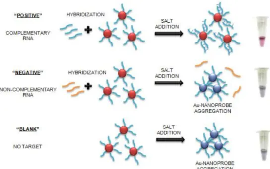
1.6.1. LSPR-based nanodiagnostics methods ... 27

1.6.2. Raman spectroscopy based nanodiagnostics methods ... 29

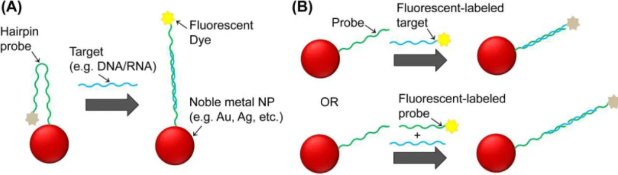
1.6.3. Fluorescence based nanodiagnostics methods ... 30

1.7. Scope of the thesis ... 32

CHAPTER 2. Materials and Methods ... 35

2.1. General Information ... 37

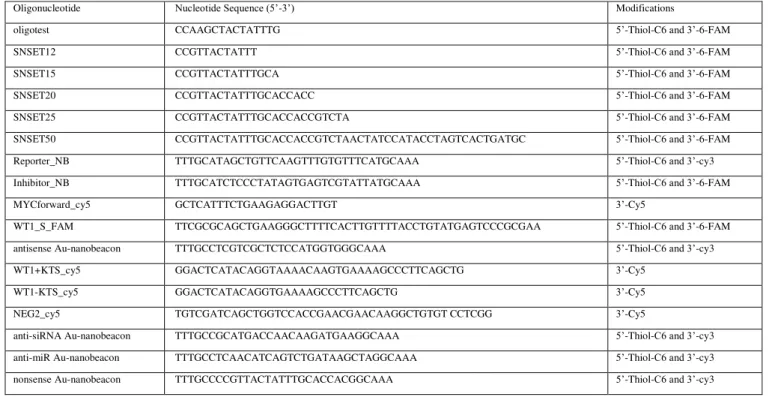
2.2. Oligonuleotides ... 38

2.3. AuNPs synthesis ... 39

2.3.1. Citrate reduction method ... 39

2.3.2. Citrate and sodium borohydride co-reduction method ... 39

2.4. AuNPs functionalisation ... 40

2.4.1. AuNPs functionalisation with fluorophores... 40

2.4.1.1. AuNPs functionalisation with SAMSA ... 40

2.4.1.1.1. Preparation of SAMSA fluorescein ... 40

2.4.1.1.2. Functionalisation of SAMSA@AuNPs surface ... 41

2.4.1.2. AuNPs modification with Rhodamine 101 and Rhodamine B ... 41

2.4.2. AuNPs functionalisation with thiolated oligonucleotides ... 41

2.4.2.1. Simple AuNPs functionalisation with thiolated oligonucleotides ... 41

2.4.2.2. Simultaneous co-functionalisation with thiolated oligonucleotides and PEG chains ... 42

2.4.2.3. Sequential co-functionalisation with PEG chains and thiolated oligonucleotides ... 42

2.5. Nanoconjugates characterization ... 43

2.5.1. AuNPs functionalisation assessment ... 43

2.5.1.1. Quantification of fluorophores at the AuNPs’ surface ... 43

2.5.1.1.1. Quantification of SAMSA on the AuNPs’ surface ... 43

2.5.1.1.2. Quantification of Rhodamine 101 and Rhodamine B on the AuNPs’ surface ... 43

xxi 2.5.1.2.1. Quantification of functionalised oligonucleotides on the AuNPs’ surface after simple

functionalisation ... 43

2.5.1.2.2. Quantification of functionalised oligonucleotides on the AuNPs’ surface after simultaneous co-functionalisation with PEG ... 44

2.5.1.2.3. Quantification of PEG chains on the AuNPs’ surface after sequential co-functionalisation with thiolated oligonucleotides ... 44

2.5.1.2.4. Quantification of functionalised oligonucleotides on the AuNPs’ surface after sequential co-functionalisation with PEG ... 45

2.5.2. Nanoconjugates physical characterization ... 45

2.5.2.1. Transmission Electron Microscopy analysis ... 45

2.5.2.2. Dynamic Light Scattering ... 45

2.5.2.3. Zeta potential analysis ... 46

2.5.2.4. Au-nanobeacon behaviour in a reductive environment ... 46

2.5.3. Photophysical characterization of the nanoconjugates ... 46

2.5.3.1. Time-dependent spectrophotometry characterization of fluorophores@AuNPs ... 46

2.5.3.1.1. Time-dependent UV/Visible Spectrophotometry of fluorophores@AuNPs ... 46

2.5.3.1.2. Time-dependent spectrofluorometry of fluorophores@AuNPs ... 46

2.5.3.2. Fluorescence quantum yields determination ... 47

2.5.3.2.1. Reference Molecules... 47

2.5.3.2.2. SAMSA@AuNPs ... 47

2.5.3.2.3. Nanoprobes ... 47

2.5.3.3. Time-resolved Fluorescence Spectroscopy Measurements ... 47

2.5.4. Au-nanobeacons specificity ... 48

2.6. Molecular and Cell Biology ... 49

2.6.1. cDNA production ... 49

2.6.1.1. RNA extraction ... 49

2.6.1.2. RT-PCR ... 49

2.6.1.2.1. Reverse Transcription ... 49

xxiii 4.1.1. Cuvette development ... 73 4.2. Absorbance interference ... 74 4.3. Emission Interference ... 77 4.4. Nanoparticle-fluorophore systems ... 77 4.4.1. Experimentally controlled reference solutions ... 79 4.4.2. Quasi-covalently bonded-fluorophores ... 79 4.4.2.1. Local pH effect and quantification of SAMSA@AuNPs ... 80 4.4.2.2. Effect of the local pH on ΦF and τF determination ... 82

4.4.2.3. Determination of kr and knr ... 82

4.4.2.4. Evaluating scattered light effect ... 86 4.4.3. Adsorbed fluorophores ... 88 4.4.3.1. Absorption of Rhodamine B at AuNPs’ surface ... 89 4.4.3.2. Absorption of Rhodamine 101 at AuNPs’ surface ... 90

4.4.3.2.1. Determination of the molar absorptivity of Rh101@AuNP ... 91 4.4.3.2.2. Fluorescence modulation of AuNPs on Rh101 ... 92 4.4.3.2.3. Determination of kr and knr of Rhodamine101@AuNPs ... 95

xxv

FIGURES INDEX

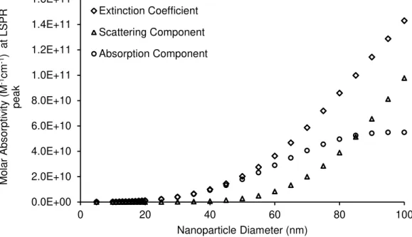
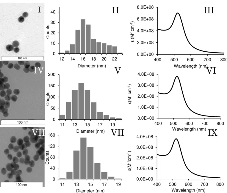
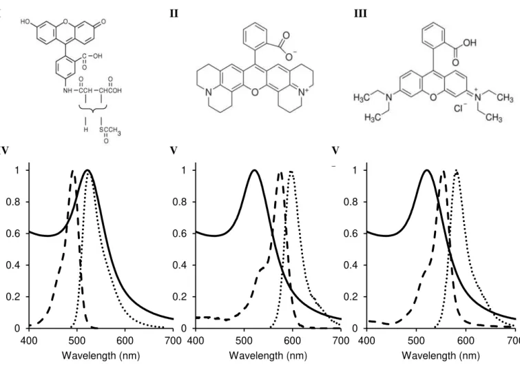
Figure 1.1. Emergence of Nanobiophotonics. ... 6 Figure 1.2. Electronic transitions during absorption. ... 7 Figure 1.3. Simplified Jablonski diagram... 9 Figure 1.4. Example of a time-correlated single photon counting decay.. ... 14 Figure 1.5. Spectral overlap between donor and acceptor. ... 17 Figure 1.6. Transfer mechanisms between donor and acceptor molecules. ... 19 Figure 1.7. LSPR of metal nanoparticles. ... 21 Figure 1.8. Cross-linking method. ... 28 Figure 1.9. Schematic representation of a non-crosslinking method. ... 29 Figure 1.10. Different approaches for fluorescent-based noble metal NPs biosensing.. ... 31 Figure 3.1. Theoretical absorption spectra of nanoparticles with different sizes. ... 64 Figure 3.2. Theoretical absorption spectra of smaller nanoparticles with different sizes. ... 64 Figure 3.3. Extinction coefficient variation with AuNPs diameter.. ... 65 Figure 3.4. Extinction coefficient variation with AuNPs diameter. ... 65 Figure 3.5. Characterization of the synthesized AuNPs. ... 69 Figure 3.6. Structure and spectra of the chosen fluorophores. ... 70 Figure 4.1. Two-compartment cuvette. ... 74 Figure 4.2. Light trasmittance through absorption cuvettes. ... 76 Figure 4.3. Differential spectra of the functionalisation of SAMSA on AuNPs. ... 76 Figure 4.4. Emission spectra of SAMSA and Rhodamine B in presence and absence of AuNPs. ... 78 Figure 4.5. Absorbance of SAMSA and SAMSA@AuNPs. ... 81 Figure 4.6. Titration of SAMSA and 5-FAM. ... 81 Figure 4.7. Absorbance of 5-FAM and SAMSA at λ=490 nm... 83 Figure 4.8. Schematic representation of the spatial dilution of scattered light from the AuNP. ... 86 Figure 4.9. Differential spectra of RhB in presence of AuNPs. ... 89 Figure 4.10. Rh101 absorption spectra over time in presence of AuNPs. ... 91 Figure 4.11. Rh101 emission spectra variation over time in presence of AuNPs. ... 93 Figure 4.12. τ and ΦF as a dependence of distance to the nanoparticle. ... 98

xxix

TABLES INDEX

Table 2.1. Unmodified oligonucleotides ... 38 Table 2.2. Oligonucleotides modified at 5’ with Thiol-C6 group and/or at 3’ with a fluorophore ... 38 Table 2.3. AuNPs synthesis reaction mixtures ... 40 Table 3.1. LSPR peak and hydrodynamic diameter of the synthesized AuNPs ... 67 Table 4.1. Experimental photophysical characterization of fluorophores in presence and absence of AuNPs. ... 80 Table 4.2. ΦF, τF, kr’ and knr’ for SAMSA@AuNP, SAMSA, 5-FAM at pH 5 and pH 8 ... 85

Table 4.3. Decay times, τ1 and τ2, and normalized pre-exponential factors, a1 and a2, for different

concentrations of Rh101 in presence of AuNPs (different AuNP:Rh101 ratios) ... 94 Table 4.4. Radiative and non-radiative rate constants of Rh101 in presence and absence of AuNPs... 95 Table 4.5. ΦF and τ for SAMSA@AuNP and SNSET probes. ... 97

2 Publications associated with this chapter:

Doria G, Conde J, Veigas B, Giestas L, Almeida C, Assunção M, Rosa J, Baptista PV (2012) Noble Metal Nanoparticles for Biosensing Applications. Sensors, 12:1657-1687

3 1.1.Background

This first segment of this thesis is intended to provide a clearer perspective on the subject in study. Before presenting the scientific background desirable for a better understanding of the work that follows, I feel it is important to provide a background of its genesis. Hopefully, this will situate the reader as to what were the motivations of the work and explain why the work in this thesis is directed to the optical properties of gold nanoparticles, fluorescence and biosensors rather than any of the numerous other potential topics in the field of nanobiophotonics.

The idea of using the modulation of fluorescence by gold nanoparticles and apply it to diagnostics and biosensing was born from an experimental setback. When I joined the laboratory, the use of gold nanoparticles for diagnostics was already a proficient topic there. The colorimetric properties of gold nanoparticles were already being used for the detection of specific DNA sequences. Simply put, DNA functionalised on gold nanoparticles would hybridise to a specific sequence that, when present, would increase the tolerance of the modified gold nanoparticles to salt-induced colour-changing aggregation. At an optimised ionic force the presence of the target sequence prevents the aggregation that occurs in its absence. Aggregation is followed by a change in the colour of the solution from red to blue.

In 2008, the colorimetric method was still being characterised and one of the main issues revolved around the identification of single nucleotide polymorphisms. This method relies on the efficiency of hybridisation between the probe and the target. When no similar sequences are in solution no hybridisation is possible and the difference between signals is clear. But the identification of sequences that differ only by one base relies on a much thinner hybridisation balance. To understand this balance it is extremely important to assess how many strands are hybridising with the probes in each case. To do this, fluorescently labelled oligonucleotides were being used and its fluorescence in solution was measured after washing. The results were arbitrary. The measurements appeared random and results had no realistic meaning, i.e., more hybridized strands than probe strands, negative amounts of hybridized strands. There was obviously something happening that was not accounted for. A clearer insight of the literature would be necessary. After a first glimpse, it was interesting to note that the randomness of the results was spread throughout literature. The available information on the effects of metal nanoparticles in fluorescence was not coherent and was even contradictory in some cases. For example, some authors defended a quenching of fluorescence while others presented enhancement.

4 molecules were from the nanoparticle was discussed as relevant to the modulation as well as the size and composition of the nanoparticles.

Further digging into the literature of metal-modulated fluorescence generated even more questions. Can fluorescence be controlled with nanoparticles? What leads to these apparently contradictory results? Can the randomness of results be controlled? Can this distance-dependence effect be used as a ruler? Is it possible to create a gold nanoparticle-fluorescence biosensor?

After meeting with my supervisors, I decided to answer these questions and enter this adventure with their guidance. The answer to these questions would not be quickly or easily answered and it would be a good but difficult challenge (especially for a biologist) that we thought to have little chance of success.

1.2.Nanotechnology, nanobiotechnology and nanobiophotonics

Nanotechnology can be described as the study and control of matter on a nanometre scale. Richard Feynman is considered to be the father of nanotechnology in his famous talk "There's plenty of room at the bottom" at an American Physical Society meeting at Caltech on December 29th, 1959 [1]. However, in the 1850’s Michael Faraday had already described the relation between colour and small size of the colloidal particles [2]. Since the 1990’s nanotechnology has boomed in terms of publications [3] by revealing the development of new materials and devices with a wide-range of applications, such as electronics, mechanics, medicine, etc. There are two main approaches for preparing nanostructures: top-down and bottom-up approaches. The top-down approach uses eroding procedures such as LASER ablation and lithography to remove and/or shape portions of larger materials. The bottom-up strategy builds the nanoparticle from molecular components, for example chemical synthesis and self-assembly.

5 Another interesting application of nanotechnology was found in biology/biotechnology creating a new field of research referred to as Nanobiotechnology. It can be considered a field that not only concerns the utilization of biological systems to produce functional nanostructures but also concerns the development and application of instruments, originally designed to generate and manipulate nanostructured materials to study fundamental biological processes and structures. Molecular diagnostics is one of the main areas that can benefit from nanobiotechnology, where the unique properties of nanomaterials and nanostructures can give rise to new techniques and methods for better diagnostics [7-9].

The cross-section between nanophotonics and nanobiotechnology creates a very specific field called nanobiophotonics that connects the application of optical properties of nanostructures and its light interacting properties with biology, biotechnology and medicine – Figure 1.1. In fact, the application of this specific field to medicine is a rapidly emerging and potentially powerful approach for disease protection, detection and treatment. The study of the underlying phenomena in nanosurface interaction mediated by biomolecules may provide insights to the development of new detection strategies able to lessen some of the current constraints in biodetection. This nanobiophotonics approach may potentiate the detection capability of biomolecules. The possibilities of this approach are almost unlimited given that minute changes to nanoparticles’ size and composition, labelling molecules or fluorophores’ properties allow for fine tuning of spectral interaction that can be used for biomolecule detection. The aim of this thesis is to understand the phenomena involved in nanosurface interaction between gold nanoparticles and fluorophores mediated by biomolecules and explore its potential as sensitive and robust biomolecular sensors.

1.3.Interaction between light and matter

Knowledge of the physical world is based on the interactions between light and matter. This dual behaviour demands the capacity to transfer energy between light and matter. This is achieved by two basic principles, the absorption of light by matter and the capacity of matter to retransform this energy back into light or to other forms of energy.

1.3.1.Light absorption

6 Figure 1.1. Emergence of Nanobiophotonics. Schematic representation of how interacting fields of science lead to Nanobiophotonics.

An electronic transition will only occur if the molecule is irradiated with light with energy corresponding to the energy gap between both states. The energies of the orbitals involved in electronic transitions have fixed values, and as energy is quantised, it would be expected that absorption peaks in spectroscopy should be sharp peaks. However, this is only rarely observed. Instead, broad absorption peaks are seen. The cause for this lies on a number of vibrational energy levels that are available at each electronic energy level, and transitions can occur to and from different vibrational levels as illustrated in Figure 1.2. The situation is further complicated by the fact that different rotational energy levels are also available to absorbing materials (omitted from Figure 1.2.). Experimentally, the efficiency of light absorption at a specific wavelength (λ) by an absorbing medium is characterized by the absorbance (A) or the transmittance (T), defined as:

( ) (Equaion 1.1) and _{( )} (Equation 1.2)

where I0_{λ and Iλ are the light intensities of the beams entering and leaving the absorbing medium,}

7 where ε(λ) is the molar absorptivity coefficient (commonly expressed in M-1_.cm-1_{), C is the}

concentration (in M or mol.dm-3_{) of absorbing species and b is the absorption path length (in cm)}

[10-13]. Failure to obey the linear dependence of the absorbance on concentration, according to the Beer– Lambert Law, may be due to aggregate formation at high concentrations or to the presence of other absorbing species. Various terms for characterizing light absorption can be found in the literature [10].

Figure 1.2. Electronic transitions during absorption. Horizontal lines represent electronic states: larger lines represent the fundamental electronic states (S0, S1 and S2) while thinner lines represent

vibrational states. Rotational states are omitted. Vertical lines represent the transition of electrons and arrows show the final state of each transition. The right part of the figure represents the correlation of the transitions with its absorption spectrum. Adapted from SpringerImages.

The molar absorption coefficient expresses the ability of a molecule to absorb light in a given solvent. The term molar absorptivity coefficient should be used instead of molar extinction coefficient in most occasions. The molar absorptivity is related to the molecular absorption cross-section (σ) which characterizes the photon-capture area of a molecule. It can be calculated as the molar absorptivity coefficient divided by the Avogadro’s number NA of molecular entities contained in a unit volume of

the absorbing medium along the light path:

σ

8 integral of the absorption band. In the quantum mechanical approach, a transition moment is presented in order to characterise the transition between an initial state and a final state. The transition moment represents the transient dipole resulting from the displacement of charges during the transition [10-13]. The use of the Beer–Lambert law deserves further attention. In practical terms, the sample is a cuvette containing a solution. The absorbance must be characteristic of the absorbing species only. Therefore, it is important to note that in the Beer–Lambert Law, the intensity of the beam entering the solution is not the intensity of the incident beam on the cuvette, and that the intensity of the beam leaving the solution is not the intensity of the beam leaving the cuvette. There usually are contributions from reflection and scattering on the cuvette walls and these walls may also absorb light. Moreover, the solvent is assumed to have no contribution, but it may also be partially responsible for a decrease in intensity because of scattering and possible absorption. The contributions of the cuvette walls and the solvent can be taken into account [10,14] by setting an appropriate reference.

1.3.2.Fluorescence

How a molecule decays from an electronic excited state back to ground state is dependent on the situation. One possible pathway is that the decay of the excited state occurs with concomitant emission of a photon. Luminescence is the emission of light from any substance. Luminescence is formally divided into two categories, fluorescence and phosphorescence. The difference between these two categories lies on the nature of the initial and final states. In fluorescence, the excited state and the ground state have the same spin multiplicity and the return to the ground-state is an allowed transition which produces a rapid emission of a photon. In phosphorescence, the spin multiplicity of the excited state and the ground state are different and the return to the ground-state is a forbidden transition which produces slow-rated emission of photon [10,11,14,15].

9 Figure 1.3. Simplified Jablonski diagram. Vertical lines represent electronic transitions and the arrows point the direction of the transition: full lines represent absorption and dashed lines represent luminescence and internal conversion. An electron in the fundamental state can be excited by incident light (hνA) which leads to an electronic transition to an excited state. In the excited state this electron

will suffer internal conversion and consequently decay to the fundamental state. This electronic transition to the fundamental state can occur non-radiatively or through luminescence: fluorescence (hνF) if the electron remains in singlet state or phosphorence (hνP) if a change in spin occurs.

The transitions between the ground state and the excited state are represented as vertical lines and show the instantaneous nature of light absorption. Transitions occur in the femtosecond time scale which, in most cases, represents a timescale too short for significant displacement of nucleus of an atom - Franck-Condon principle. Another general property of fluorescence is that the same fluorescence emission spectrum is generally observed irrespective of the excitation wavelength. This is known as Kasha's rule [16], even though Vavilov had previously reported (in 1926) that quantum yields were generally independent of excitation wavelength [17]. Upon excitation into higher electronic and vibrational levels, the excess energy is quickly dissipated, leaving the fluorophore in the lowest vibrational level of S1. This relaxation takes approximately 1 ps. Because of this rapid relaxation, emission spectra are usually independent of the excitation wavelength.

Analytically, the decay of an excited state to the ground state can be expressed as a decay rate. This rate is the sum of the rates associated to each pathway that the excited molecule can take. Therefore a radiative rate (kr) can be established as the rate at which a molecule decays to the ground state with

10 purposes, in fluorescence studies, all the non-radiative pathways’ constants are usually summed up in one single non-radiative constant (knr).

1.3.2.1.Steady-state and Time-resolved fluorescence

Fluorescence measurements can be broadly classified into two types of measurement: steady-state and time-resolved. Steady-state measurements, the most common type, are performed with constant illumination and observation. The sample is illuminated with a continuous beam of light, and the intensity or emission spectrum is recorded. Because of the nanosecond timescale of fluorescence, most measurements are steady-state measurements. When the sample is first exposed to light, steady state is reached almost immediately. The second type of measurement is time-resolved which is used for measuring intensity decays. For these measurements the sample is exposed to a pulse of light, where the pulse width is typically shorter than the decay time of the sample. The intensity decay is recorded with a high-speed detection system that permits the intensity to be measured on the nanosecond, picosecond and even femtosecond [18-20] timescale. It is important to understand the relationship between steady-state and time-resolved measurements. A steady-state observation is simply an average of the time-resolved phenomena over the intensity decay of the sample [10].

1.3.2.2.Fluorescence Quantum yields and Lifetimes

The fluorescence quantum yield (ΦF) and lifetime (τ) are perhaps the most important characteristics of

a fluorophore. The fluorescence quantum yield is the number of emitted photons relative to the number of absorbed photons. Substances with the largest quantum yields, approaching unity, such as rhodamine molecules, display the brightest emissions. The lifetime is also important as it represents the time available for the excited fluorophore to interact with other components of the system or diffuse in its environment.

The fluorescence quantum yield is the ratio of the number of photons emitted to the number absorbed. Both radiative and non-radiative pathways will depopulate the excited state and account to the amount of excited states formed (amount of absorbed light). The fraction of fluorophores that decay through emission, and hence the quantum yield, is given by:

Φ

(Equation 1.5)

11 The lifetime of the excited state is defined by the average time the molecule spends in the excited state prior to return to the ground state. Logically, the smaller the excited-state lifetime the higher is the associated rate, hence:

(Equation 1.6)

Fluorescence emission is a random process, and few molecules emit their photons at precisely t = τ. The lifetime is an average value of the time spent in the excited state which means that for an exponential decay 63% of the molecules have decayed prior to t = τ and 37% decay at t > τ.

The quantum yield and lifetime of the molecules can be modified by factors that affect either of the rate constants (kr or knr). Scintillators are generally chosen for their high quantum yields. These high

yields are a result of large kr values when compared to the knr [10,11,14].

1.3.2.3.Determination of fluorescence quantum yields

The fluorescence quantum yield is related to the efficiency of the fluorescence process. It is defined as the ratio between the number of emitted photons to the number of absorbed photons. The maximum fluorescence quantum yield is 1, which would mean that every absorbed photon results in an emitted photon. Hence, by definition the fluorescence quantum yield is:

Φ

Although this expression is analytically less practical than Equation 1.7, experimentally, it is clearer in what is needed to determine the fluorescence quantum yield – a quantification of both absorbed and emitted photons. The determination of fluorescence quantum yields is usually associated with high errors due to several technical issues that can occur. For this reason, several methods were developed which can be divided into either absolute or relative methods [11].

Absolute quantum yield determination methods will present a result that is dependent on the technical conditions of its determination. Among the most popular are the integrated sphere method, calorimetric method and light scattering methods.

12 Calorimetric methods rely on the changes observed in temperature or volume during irradiation. The basic principle of this approach is the comparison of the observed changes of a non-luminescent molecule and a fluorescent sample with comparable optical densities. The non-luminescent molecule will have a quantum yield of zero, and so, the ratio of the temperature variations in the two solutions provides the fraction of the absorbed energy which is lost non-radiatively in the fluorescent sample. This value is complementary to the fluorescence quantum yield [22].

Light scattering methods rely on molecules that behave as substances that reemit all the photons irradiated upon them without change in wavelength. These molecules are usually called ideal scatterers. Although no absorption or emission occurs, ideal scatterers behave as if they had a quantum yield of 1. The fluorescence quantum yield can then be determined by comparing a molecule’s fluorescence with the intensity of light due to Rayleigh scattering from the ideal scatterer solutions with the fluorescence of the sample solutions at the same wavelength [23]. Correction factors have to be introduced in order to account for the different spatial distribution of light from the scattering and fluorescent solutions due to the polarized scattered light and unpolarized fluorescence [24]. Relative quantum yields determination methods are based on the assumption that if two molecules are studied in the same apparatus, absorb the same amount of light, the integrated areas under their corrected fluorescence spectra will be proportional to their fluorescence quantum yields. As such, the relation between quantum yields and fluorescence intensity of two molecules can be expressed as:

(Equation 1.8)

where ΦF represents the quantum yields and A represents absorbance at the respective excitation

wavelengths. One very important factor for a proper quantum yield calculation using this method is the choice of the adequate reference molecule. Reference molecules should present specific properties in order to be more adequate. The most important of the aspects to take into account are the emission properties of the molecule. The reference molecule should have a broad spectrum with no fine structure and have a high fluorescence quantum yield. Small overlap between absorption and emission spectra is also favourable as it reduces the possibility of self-absorption. The reference and the sample should present similar absorption spectra in order to facilitate the matching of the absorbance of both molecules. For all the presented reasons, it requires a series of suitable reference materials to cover the light spectrum in the visible region [11].

13 concentrations, correction factors must be applied. Working in lower concentrations may also avoid self-absorption in cases where a significant overlap between the absorption and emission spectra exists. Refractive index issues may also rise when reference molecules and sample molecules present different solution optical geometry. The errors due to refractive index changes may exist when the radiation passes from a high to a lower refractive index or by internal reflection of emitted light within the cuvette at all interfaces between zones of different refractive indices. These errors are especially relevant if reference and sample are in different solvents [25]. Other factors such as temperature, polarization of light or photostability may also affect the fluorescence quantum yield determination [11].

1.3.2.4.Determination of fluorescence lifetimes

Prior to further discussion of lifetime measurements, it is important to take another look at the meaning of τ. Consider a sample containing the fluorophore that is excited with an infinitely sharp pulse of light. This excitation results in an initial population (n0) of fluorophores in the excited state.

The excited-state population decays with a rate kr + knr according to:

( )

(

where n(t) is the number of excited molecules at time t following excitation. Emission is a random event, and each excited fluorophore has the same probability of emitting in a given period of time. This results in an exponential decay of the excited state population:

( )

What is observed in a fluorescence experiment is fluorescence intensity. In turn, this intensity is proportional to n(t) [10,13]. Hence, the equation above can also be written in terms of the time-dependent intensity I(t). Integration of Equation 1.10 with the intensity substituted for the number of molecules yields the usual expression for a single exponential decay:

( )

where I0 is the intensity at time 0. The inverse of the lifetime is the sum of the rates which depopulate

the excited state and so the fluorescence lifetime can be determined from the slope of a plot of log I(t) versus t, but more commonly by fitting the data to assumed decay models. The lifetime is the average amount of time a fluorophore remains in the excited state following excitation. A typical result is represented in Figure 1.4. This can be experimentally assessed by pulse fluorometry.

14 (TCSPC) method. The basic principle of TCSPC is the probability of detecting a single photon at time t after an exciting pulse is proportional to the fluorescence intensity at that time. After timing and recording the single photons following a large number of exciting pulses, the fluorescence intensity decay curve can be reconstructed.

Figure 1.4. Example of a time-correlated single photon counting decay. Representative time-correlated single photon counting decay (black circles) for ATTO 465 in H2O at 25 ˚C (excitation at λ=297 nm, detection at λ=510 nm) [26]. Each circle represents the time taken by one photon to reach the detector since the sample was excited. The linear representations represent the best possible fitting to the experimental points. τ is obtained from the equation of this linear representation.

15 the histogram of pulse heights represents the fluorescence decay curve. The larger the number of events, the better the accuracy of the decay curve. When deconvolution is required, the time profile of the exciting pulse is recorded under the same conditions by replacing the sample with a scattering solution (Ludox – colloidal silica – or glycogen) [10,14].

The excitation source is of major importance. Flash lamps running in air, or filled with N2, H2 or D2

are not expensive but the excitation wavelengths are restricted to the 200–400 nm range. These deliver nanosecond pulses so that decay times of a few hundreds of picoseconds can be measured. Furthermore, the repetition rate is not high and because the number of fluorescence pulses per exciting pulse must be kept below 5%, the collection period may be quite long, depending on the required accuracy (a few tens of minutes to several hours). For long collection periods, lamp drift may become a problem. Lasers as excitation sources are of course much more efficient and versatile but much more expensive. The pulse widths are in the picosecond range with a high repetition rate. This rate must be limited to a few MHz in order to let the fluorescence of long lifetime samples vanish before a new exciting pulse is generated. Synchrotron radiation can also be used as an excitation source with the advantage of almost constant intensity versus wavelength over a very broad range, but the pulse width is in general of the order of hundreds of picosecond or not much less. The time resolution of the instrument is governed not only by the pulse width but also by the electronics and the detector. The linear time response of the TAC is most critical for obtaining accurate fluorescence decays. The response is more linear when the time during which the TAC is in operation and unable to respond to another signal is minimized. For this reason, it is better to collect the data in the reverse configuration: the fluorescence pulse acts as the start pulse and the corresponding excitation pulse as the stop pulse. In this way, only a small fraction of start pulses result in stop pulses and the collection statistics are better. Microchannel plate photomultipliers are preferred to standard photomultipliers, but they are much more expensive. They exhibit faster time responses and do not show a significant colour effect. With mode-locked lasers and microchannel plate photomultipliers, the instrument response in terms of pulse width is 30–40 ps so that decay times as short as 3–4 ps can be measured [10,14].

1.3.2.5.Fluorescence Intensity Quenching

16 Collisional quenching occurs when the excited-state fluorophore is deactivated upon contact with some other molecule in solution, usually called quencher. The fluorophore returns to the ground state during an encounter with the quencher but the molecules are not chemically changed in the process. A wide variety of molecules can act as collisional quenchers. Examples include oxygen, halogens, amines, and electron-deficient molecules like acrylamide. The mechanism of quenching varies with the fluorophore–quencher pair. For example, quenching of indole by acrylamide is probably due to electron transfer from indole to acrylamide, which does not occur in the ground state [11]. Quenching by halogen and heavy atoms occurs due to spin–orbit coupling and intersystem crossing to the triplet state [33].

Static quenching or contact quenching, on the other hand, occurs when the molecules form a complex before excitation occurs. The complex has its own unique (non)fluorescence and absorption properties. For example, static quenching often occurs when, due to hydrophobic effects, dyes stack together to minimize contact with water and consequently form aggregates. Planar aromatic dyes that are matched for association through hydrophobic forces can enhance static quenching [14,34,35].

1.3.2.6.Energy Transfer and Electron transfer

Fluorescence intensity can also decrease when a molecule transfers energy to another molecule in its vicinity – energy transfer. Although energy transfer is usually not considered to be quenching, in the general sense energy transfer results in the decrease of fluorescence intensity of the donor excited molecule.

17 Figure 1.5. Spectral overlap between donor and acceptor. The spectral overlap between the emission spectrum of the donor (a – CdTe quantum dots in this case) and the absorption spectrum of the acceptor (b – neutral red in this case) represents the likeliness with which the energy from an excited electron in the donor will be transferred to the acceptor [37].

The rate of energy transfer kT(r) can be expressed as:

( )

(

)

where r is the distance between the donor and acceptor and τD is the lifetime of the donor in the

absence of energy transfer. The efficiency of energy transfer for a single donor–acceptor pair at a fixed distance is described below:

E

Hence the extent of transfer depends on the sixth power of the distance. Fortunately, the Förster distances are comparable in size to biological macromolecules: 20 to 60 Å. For this reason energy transfer has been used as a "spectroscopic ruler" for measurements of distance between sites on proteins [38]. The theory is adjusted for donors and acceptors that are covalently linked, free in solution, or contained in the restricted geometries of membranes or DNA. Additionally, depending on donor lifetime, diffusion can increase the extent of energy transfer [14].

18 The complexity of FRET is best understood by considering a single donor and acceptor separated by a distance (r). The rate of transfer for a donor and acceptor separated by a distance r is given by:

( )

(

) ∫

( )

( )

Where ΦD is the quantum yield of the donor in the absence of acceptor, n is the refractive index of the

medium, NA is de Avogadro’s number, r is the distance between the donor and acceptor, τD is the

lifetime of the donor in the absence of acceptor, FD(λ) is the corrected fluorescence intensity of the

donor in the wavelength range with the total intensity (area under the curve) normalized to the unity, ε(λ) is the absorption spectra of the acceptor in extinction coefficient units (in typical units of M-1_.cm -1_{), k}2 _{is the dipole orientator factor – usually assumed to be 2/3 as a dynamic random averaging of the}

donor and acceptor. The integral term, also represented as J(λ), corresponds to the spectral overlap between the donor emission and acceptor absorption spectra [14,39].

In practical terms, it is easier to assess the data when it is represented in distances than in transfer rates. So, by assuming that half the donor molecules will decay energy transfer and the other half will decay normally (radiative and non-radiative pathways), R0 can be estimated as:

( )

∫ ( ) ( )

Once R0 is known, the rate of energy transfer can be easily calculated (Equation 1.12) as well as the

efficiency of energy transfer (Equation 1.13) for a given distance. Using these equations and knowing k2_{, n, Φ}

D and J(λ) and, consequently, R0, it is possible to calculate the distance between a given pair of

donor and acceptor.

19 In most donor-fluorophore–quencher-acceptor situations, the Förster mechanism is more important than the Dexter mechanism. With both Förster and Dexter energy transfer, the shapes of the absorption and fluorescence spectra of the dyes are unchanged [14]. The electronic transitions are the same as when the molecules are isolated. Neither Förster nor Dexter mechanisms imply any chemical change in donor or acceptor. On the contrary, both mechanisms only cause the donor molecule to deactivate its’ excited state and the acceptor molecule to go from the fundamental state to an excited state. Figure 1.6 schematically resumes both Förster and Dexter mechanisms.

Figure 1.6. Transfer mechanisms between donor and acceptor molecules. Förster resonance energy transfer promotes the deactivation of the excited state of the donor by transferring the energy to the acceptor which, in turn, goes to the excited state. Dexter mechanism does not involve the direct deactivation of the donor excited state rather transferring the excited electron to the acceptor while a fundamental state electron of the acceptor is transferred back to the donor.

1.4.Nanoparticles

Nanoparticle as a term refers to a particle with size comprehended between a few and hundreds of nanometres (10-9 _{m). These can be composed of one or more inorganic compounds, such as noble}

20 nanocrystals, surface plasmon resonance in some metal nanoparticles and superparamagnetism in magnetic materials [41].

Numerous techniques have been developed to synthesize noble metal nanoparticles, including chemical methods (e.g., chemical reduction, photochemical reduction, co-precipitation, thermal decomposition, hydrolysis, etc.) and physical methods (e.g., vapour deposition, laser ablation, grinding, etc.), whose ultimate goal is to obtain nanoparticles with a good level of homogeneity and provide fine control over size, shape and surface properties, in order to better take advantage of their unique physicochemical properties [41].

Metal nanoparticles have size-dependent optical properties that have been explored in many biological applications, such as in medicine and molecular diagnostics. Gold nanoparticles (AuNPs) are among the most extensively studied nanomaterials and have led to the development of various techniques and methods for molecular diagnostics, imaging, drug delivery and therapeutics [42-45]. Metal nanoparticles (including AuNPs) also present significant electronic properties, such as charge storage and conductivity [46] which have been used in memory devices [47-49] and molecular switches [50], and catalytic activity [3,51,52], a property not observed in the bulk material.

AuNPs can be easily synthesized in sizes ranging between 3 and 200 nm in diameter and in different shapes. The most common AuNPs are quasi-spherically shaped, mainly due to their surface energy that favours the formation of spherical particles. One of the most common methods used to synthesize quasi-spherical AuNPs is the chemical reduction of Au(III) to Au(0) ions using sodium citrate as a reducing agent, a method first developed by Turkevich [53] and latter optimized by Frens [54]. In this approach, the citrate acts both as reducing agent and as capping agent which, as the AuNPs form, prevents the nanoparticles from forming larger particles and simultaneously conferring them a mild stability due to electrostatic repulsion between citrate-capped AuNPs [55]. Recent modifications of the Turkevich method have allowed a better distribution and control over the size of the AuNPs, where a range between 9–120 nm can be achieved just by varying the citrate/Au ratio [52,56,57]. Alternatively, many other aqueous- and organic-based methodologies have been developed for the controlled synthesis of different noble metal nanoparticles, including spherical or non-spherical, pure, alloy or core/shell nanoparticles of gold, silver, platinum, palladium and/or rhodium [58-60].

1.4.1.Localized Surface Plasmon Resonance

21 consequently dispersing secondary radiation in all directions. The LSPR presents them with exceptionally high absorption coefficients and scattering properties that allow for higher sensitivity in optical detection methods than conventional organic dyes [62]. AuNP solutions have an intense red colour, which changes to brown when the particles are small (<2 nm) and to violet in the case of bigger nanoparticles. The red colour originates from absorption or scattering of light around 520 nm by localized surface plasmons. Because the particles strongly interact with green light, they appear red. Surface plasmon band arises from collective movements of free electrons, which can follow oscillations of an electric field. The electric field of incident light couples with the conduction band electrons and polarizes them relative to the centre of mass of the nanoparticle [63]. This leads to a charge difference between the opposite surfaces of the nanoparticle, which then acts as a restoring force and causes dipolar oscillation of the electrons [63]. This interaction is schematically represented in Figure 1.7.

Figure 1.7. LSPR of metal nanoparticles. Schematic representation of how the interaction of the electromagnetic waves with the metal NPs surface electrons generates a surface plasmon resonance [64].

22 approaches have been made to calculate the absorption and scattering efficiencies as well as the extinction coefficient of AuNPs with different sizes and shapes [62].

1.4.2.Other optical properties

Excitation of AuNPs with short laser pulses increases the energy of the electrons. In order to return to their initial state, the electrons have to lose the gained energy either as heat (phonons) or as light (photons). Relaxation of the excited gold nanoparticles without emission of photons proceeds through three steps. First, the high temperature electrons distribute their energy among all the electrons by electron-electron scattering in less than a picosecond [73,74]. Second, energy is transferred from electrons to the whole particle via electron-phonon scattering during a few picoseconds [75,76]. The transfer of heat from the nanoparticle to the surrounding medium via phonon-phonon scattering is the third step, which proceeds in hundreds of picoseconds [75,76]. The relaxation time constants are dependent on the excitation energy [77,78], excitation wavelength [73] and surrounding medium [79]. An alternative pathway for relaxation of excited electrons in gold nanoparticles is photon emission [80,81].

1.4.3.Nanoparticle functionalisation

The development of new biosensing and therapeutic applications based on AuNPs has been pushing forward the chemistry for their functionalisation with different moieties such as nucleic acids, antibodies, biocompatible polymers, enzymes and other proteins, in a quest for an increased biocompatibility and targeting specificity [82,83].

23 1.5.Gold nanoparticle-fluorophore systems

Molecular fluorophores in the vicinity of isolated colloidal metal nanoparticles usually experience modulation of their emission and, consequently, of the observable fluorescence [90-92]. Metal nanoparticles can modulate the optical properties of molecules near their metal surfaces, including changes to the radiative and non-radiative rate constants [93,94]. In the case of a fluorophore’s emission, nanoparticles have even been proposed both as enhancers and as quenchers [95,96].

1.5.1.Molecular interactions in gold nanoparticle-fluorophore systems

The vicinity of a metal nanoparticle to the photoexcited fluorophore can affect the relaxation of the fluorophore at least via three processes: electron transfer, energy transfer and modification of the radiative rate of the fluorophore. Energy and electron transfer are both non-radiative relaxation routes that become available for the fluorophore when combined with gold nanoparticles. Assuming all three possible pathways can occur simultaneously, then whether enhancement or quenching is observable depends on the balance between changes in radiative vs. non-radiative (including temperature dependent vibrational dumping and energy transfer) and photochemical pathways (e.g., photo-induced electron transfer) [95-97].

1.5.2.Electron transfer mechanisms

Pyrene-functionalised gold nanoparticles were the first gold nanoparticle-based systems for which photoinduced electron transfer was described [84]. In this case, electron transfer takes place from photoexcited pyrenes to 2-3 nm gold nanoparticles. However, this requires a small distance between the nanoparticle and the pyrene molecules [98]. Chlorophyll molecules assembled electrostatically on 8 nm nanoparticles transfer electrons to the particles after photoexcitation [99]. In these systems, close proximity between nanoparticles and fluorescent molecules is required for the electron transfer to take place.

1.5.3.Energy transfer systems

24 According to the Fermi Golden Rule [101] in the dipole approximation of energy transfer, the energy transfer rate is related to a product of the interaction elements of the donor and the acceptor. A single dipole’s interaction elements are dependent on 1/r3_{. Then, on one hand, FRET occurs between two}

independent and isolated dipoles which derives into an interaction dependent with (1/r3_)(1/r3_)=1/r6 _as

was described in the previous subchapters. On the other hand, if the interaction occurs between a planar structure (2D dipole array) and an isolated dipole, then the distance dependence becomes associated to (1/r)(1/r3_)=1/r4 _[87,101].

FRET between two dipoles can be applied in principle to gold nanoparticle-fluorophore energy transfer. Experiments have shown that energy transfer in systems with gold nanoparticles can range up to 20 nm [102], which is beyond the usual Forster range. An alternative way to face these systems is to treat the fluorophore as a dipole and the gold nanoparticle as a surface, which would lead to a 1/r4

dependence of energy transfer rate. This mechanism has been called (nano)-surface energy transfer or (N)SET and has been applied to several fluorophore-gold nanoparticle systems [102,103]. This alternative resembles with typical FRET but R0 is determined from different physical parameters:

quantum yield, the frequency of donor electronic transition, Fermi frequency and wave vector of the metal [102].

Most of this discussion has been shortened into how the experimental results match the theoretical energy transfer rates of FRET or NSET. This problem has been posed in a single common equation, very similar to Equation 1.13 but more ambiguous:

E

where n=6 means a typical FRET scenario and n=4 means a SET system.

1.5.4.Radiative-rate changes

25 1.5.5.Main theoretical approaches on radiative and non-radiative modulation

One of the first models to predict the effect of small dielectric particles on the spectroscopic properties of molecules interacting with them was published by Joel Gersten and Abraham Nitzan in 1981 [93]. The Gersten-Nitzan model predicts the theoretical expressions for the quantum yields, radiative and non-radiative decay rates under the assumption that the nanoparticles are much smaller than the wavelength. The prediction is valid for different sizes, shapes and dielectric constant, which can relate both with the composition of the nanoparticle and the medium. The most important issues taken into account by this model include the total dipole of the system (and not only the nanoparticle), the possible additional induced dipole caused by the presence of the nanoparticle and the relative position of the transition moment relatively to the surface of the nanoparticle (whether they are parallel or perpendicular). One very important issue raised by this model is the complete dependence of the behaviour on the shape, size and dielectric constant of the nanoparticle. Also, it calls attention to the major difference observed when comparing free fluorophores with fluorophores interacting with metal structures and even when comparing between fluorophores interacting with nanoparticles and plane surfaces. The Gersten-Nitzan model is the most used model when studying nanoparticle-fluorophore systems.

Another famous model for nanoparticle-fluorophore systems was proposed by Persson and Lang [106] in 1982 improving an earlier attempt by Chance, Prock and Silbey [94] to analyse similar situations using electrodynamics. Unlike what happens in Gersten-Nitzan model, this model describes the electron-hole pair quenching of excited states near a metal. Instead of considering the effect of a nanoparticle in the excited-state of a molecule it simply assumes the difference in sizes between nanoparticles and fluorophores is so big that the nanoparticles behave as if they were a planar metal structure. Under these assumptions, the dipole is considered to interact with conduction band electrons of the metal, which, in turn, are assumed to move freely in a semi-infinite background. This is the first model to discuss the theoretical modelling on the distance dependence of the nanoparticle-fluorophore interaction as being modulated with 1/r4 _{by a metallic surface.}