Introduction
This chapter provides an introduction to the analysis of networks through the presen-tation of several examples of research. This provides not only some idea of why the subject is interesting, but also of the range of networks studied, approaches taken and methods used.
1.1
Why Model Networks?
Social networks permeate our social and economic lives. They play a central role in the transmission of information about job opportunities, and are critical to the trade of many goods and services. They are the basis of the provision of mutual insurance in developing countries. Social networks are also important in determining how diseases spread, which products we buy, which languages we speak, how we vote, as well as whether or not we decide to become criminals, how much education we obtain, and our likelihood of succeeding professionally. The countless ways in which network structures a¤ect our well-being make it critical to understand: (i) how social network structures impact behavior, and (ii) which network structures are likely to emerge in a society. The purpose of this monograph is to provide a framework for an analysis of social networks, with an eye on these two questions.
As the modeling of networks comes from varied …elds and employs a variety of di¤erent techniques, before jumping into formal de…nitions and models, it is useful to start with a few examples that help give some impression of what social networks are and how they have been modeled. The following examples illustrate widely di¤erent perspectives, issues, and approaches; previewing some of the breadth of the range of
topics to follow.
1.2
A Set of Examples:
The …rst example is a detailed look at the role of social networks in the rise of the Medici.
1.2.1
Florentine Marriages
The Medici have been called the “godfathers of the Renaissance.” Their accumulation of power in the early …fteenth century in Florence, was orchestrated by Cosimo de’ Medici despite the fact that his family started with less wealth and political clout than other families in the oligarchy that ruled Florence at the time. Cosimo consolidated political and economic power by leveraging the central position of the Medici in net-works of family inter-marriages, economic relationships, and political patronage. His understanding of and fortuitous position in these social networks enabled him to build and control an early forerunner to a political party, while other important families of the time ‡oundered in response.1
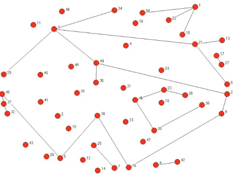
Padgett and Ansell [493] provide powerful evidence for this by documenting the network of marriages between some key families in Florence in the 1430’s. The following …gure provides the links between the key families in Florence at that time, where a link represents a marriage between members of the two linked families.2
As mentioned above, during this time period the Medici (with Cosimo de’ Medici playing the key role) rose in power and largely consolidated control of the business and politics of Florence. Previously Florence had been ruled by an oligarchy of elite families. If one examines wealth and political clout, however, the Medici did not stand out at this point and so one has to look at the structure of social relationships to understand why it was the Medici who rose in power. For instance, the Strozzi had
1See Kent [369] and Padgett and Ansell [493] for detailed analyses, as well as more discussion of
this example.
2The data here were originally collected by Kent [369], but were …rst coded by Padgett and Ansell
Figure 1.1: 15th Century Florentine Marriges Data from Padgett and Ansell [493] (drawn using UCINET)
both greater wealth and more seats in the local legislature, and yet the Medici rose to eclipse them. The key to understanding this, as Padgett and Ansell [493] detail, can be seen in the network structure.
If we do a rough calculation of importance in the network, simply by counting how many families a given family is linked to through marriages, then the Medici do come out on top. However, they only edge out the next highest families, the Strozzi and the Guadagni, by a ratio of 3 to 2. While this is suggestive, it is not so dramatic as to be telling. We need to look a bit closer at the network structure to get a better handle on a key to the success of the Medici. In particular, the following measure of betweenness is illuminating.
Let P(ij) denote the number of shortest paths connecting family i to family j. 3
Let Pk(ij) denote the number of these paths that family k lies on. For instance, the
shortest path between the Barbadori and Guadagni has three links in it. There are
3Formal de…nitions of path and some other terms used in this chapter appear in Chapter 2. The
two such paths: Barbadori Medici Albizzi Guadagni, and Barbadori Medici -Tournabouni - Guadagni. If we set i= Barbadori and j = Guadagni, then P(ij) = 2. As the Medici lie on both paths,Pk(ij) = 2when we setk=Medici, andi=Barbadori
and j = Guadagni. In contrast this number is 0 if we set k = Strozzi, and is 1 if we set k = Albizzi. Thus, in a sense, the Medici are the key family in connecting the Barbadori to the Guadagni.
In order to get a fuller feel for how central a family is, we can look at an average of this betweenness calculation. We can ask for each pair of other families, what fraction of the total number of shortest paths between the two the given family lies on. This would be 1 if we are looking at the fraction of the shortest paths the Medici lie on between the Barbadori and Guadagni, and 1/2 if we examine the corresponding fraction that the Albizzi lie on. Averaging across all pairs of other families gives us a sort of betweenness or power measure (due to Freeman [239]) for a given family. In particular, we can calculate
X
ij:i6=j;k =2fi;jg
Pk(ij)=P(ij)
(n 1)(n 2)=2 (1.1)
for each family k, where we set Pk(ij)
P(ij) = 0 if there are no paths connecting i and
j, and the denominator captures that a given family could lie on paths between up to (n 1)(n 2)=2 pairs of other families. This measure of betweenness for the Medici is .522. That means that if we look at all the shortest paths between various families (other than the Medici) in this network, the Medici lie on over half of them! In contrast, a similar calculation for the Strozzi comes out at .103, or just over ten percent. The second highest family in terms of betweenness after the Medici is the Guadagni with a betweenness of .255. To the extent that marriage relationships were keys to communicating information, brokering business deals, and reaching political decisions, the Medici were much better positioned than other families, at least according to this notion of betweenness.4 While aided by circumstance (for instance, …scal problems
resulting from wars), it was the Medici and not some other family that ended up consolidating power. As Padgett and Ansell [493] put it, “Medician political control was produced by network disjunctures within the elite, which the Medici alone spanned.”
4The calculations here are conducted on a subset of key families (a data set from Wasserman and
This analysis shows that network structure can provide important insights beyond those found in other political and economic characteristics. The example also illustrates that the network structure is important beyond a simple count of how many social ties each member has, and suggests that di¤erent measures of betweenness or centrality will capture di¤erent aspects of network structure.
This example also suggests a series of other questions that we will be addressing throughout this book. For instance, was it simply by chance that the Medici came to have such a special position in the network or was it by choice and careful plan-ning? As Padgett and Ansell [493] say (footnote 13), “The modern reader may need reminding that all of the elite marriages recorded here were arranged by patriarchs (or their equivalents) in the two families. Intra-elite marriages were conceived of partially in political alliance terms.” With this perspective in mind we then might ask why other families did not form more ties, or try to circumvent the central position of the Medici. We could also ask whether the resulting network was optimal from a variety of perspectives: was it optimal from the Medici’s perspective, was it optimal from the oligarchs’ perspective, and was it optimal for the functioning of local politics and the economy of 15th century Florence? These types of questions are ones that we can begin to answer through explicit models of the costs and bene…ts of networks, as well as models of how networks form.
1.2.2
Friendships Among High School Students
The next example comes from the The National Longitudinal Adolescent Health Data Set, known as “Add Health.”5 These data provide detailed social network information
for over ninety thousand high school students from U.S. high schools interviewed during the mid 1990s; together with various data on the students’ socio-economic background, behaviors and opinions. The data provide a number of insights and illustrate some features of networks that are discussed in more detail in the coming chapters.
Figure 1.2 shows a network of romantic relationships as found through surveys of
5Add Health is a program project designed by J. Richard Udry, Peter S. Bearman, and Kathleen
students in one of the high schools in the study. The students were asked to list the romantic liaisons that they had during the six months previous to the survey.
Figure 1.2: A Figure from Bearman, Moody and Stovel [47] based the Add Health Data Set. A Link Denotes a Romantic Relationship, and the Numbers by Some Components Indicate How Many Such Components Appear.
There are several things to remark about Figure 1.2. The network is nearly a
the giant component, and then a couple of smaller cycles present, but very few overall. The absence of many cycles means that as one walks along the links of the network until hitting a dead-end, most of the nodes that are met are new ones that have not been encountered before. This is important in navigation of networks. This feature is found in many random networks in cases where there are enough links so that a giant component is present, but there are also few enough links so that the network is not fully connected. This contrasts with what we see in the denser friendship network pictured in Figure 1.3, where there are many cycles, and a shorter distance between nodes.
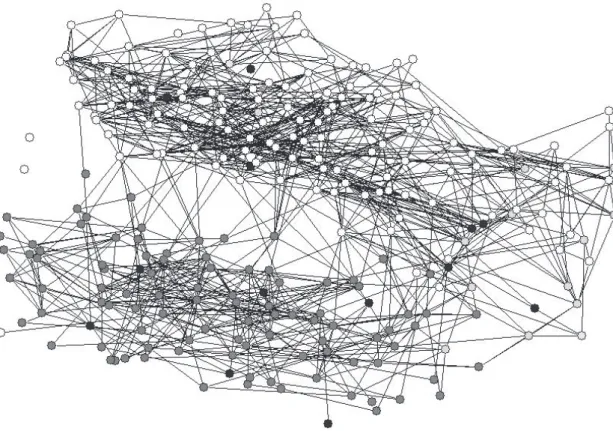
The network pictured in Figure 1.3 is also from the Add Health data set and con-nects a population of high school students.6 Here the nodes are coded by their race
rather than sex, and the relationships are friendships rather than romantic relation-ships. This is a much denser network than the romance network, and also exhibits some other features of interest.
A strong feature present in Figure 1.3 is what is known as “homophily,” a term due to Lazarsfeld and Merton [406]. That is, there is a bias in friendships towards similar individuals; in this case the homophily concerns the race of the individuals. This bias is above what one would expect due to the makeup of the population. In this school, 52 percent of the students are white and yet 86 percent of whites’ friendships are with other whites. Similarly, 38 percent of the students are black and yet 85 percent of blacks’ friendships are with other blacks. Hispanics are more integrated in this school, comprising 5 percent of the population, but having only 2 percent of their friendships with Hispanics.7 If friendships were formed without race being a factor,
then whites would have roughly 52 percent of their friendships with other whites rather than 85 percent.8 This bias is referred to as “inbreeding homophily” and has strong
consequences. As we can see in the …gure, it means that the students end up somewhat
6A link indicates that at least one of the two students named the other as a friend in the survey.
Not all friendships were reported by both students. For more detailed discussion of these particular data see Curarrini, Jackson and Pin [173].
7The Hispanics in this school are exceptional compared to what is generally observed in the larger
data set of 84 high schools. Most racial groups (including Hispanics in many of the other schools) tend to have a greater percentage of own-race friendships than the percentage their race in the population, regardless of their fraction of the population. See Currarini, Jackson and Pin [173] for details.
8There are a variety of possible reasons for the patterns observed, as it could be that race is
Figure 1.3: “Add Health” Friendships among High School Students Coded by Race: Hispanic=Black, White=White, Black=Grey, Asian and Other = Light Grey.
segregated by race, and this will impact the spread of information, learning, and the speed with which things propagate through the network; themes that are explored in detail in what follows.
1.2.3
Random Graphs and Networks
The examples of Florentine marriages and high school friendships suggest the need for models of how and why networks form as they do. The last two examples in this chapter illustrate two complementary approaches to modeling network formation.
mathematics, and has recently been extended in various directions by the computer science, statistical physics, and economics literatures (as will be examined in some of the following chapters). This is perhaps the most basic model of network formation that one could imagine: it simply supposes that a completely random process is responsible for the formation of the links in a network. The properties of such random networks provide some insight into the properties that some social and economic networks have. Some of the properties that have been extensively studied are how links are distributed across di¤erent nodes, how connected the network is in terms of being able to …nd paths from one node to another, what the average and maximal path lengths are, how many isolated nodes there are, and so forth. Such random networks will serve as a very useful benchmark against which we can contrast observed networks; as such comparisons help identify which elements of social structure are not the result of mere randomness, but must be traced to other factors.
Erdös and Rényi [213], [214], [215] provided seminal studies of purely random net-works.9 To describe one of the key models, …x a set of n nodes. Each link is formed
with a given probability p, and the formation is independent across links.10 Let us
examine this model in some detail, as it has an intuitive structure and has been a springboard for many recent models.
Consider a set of nodes N = f1; : : : ; ng, and let a link between any two nodes, i
andj, be formed with probability p, where 0< p <1. The formation of links is inde-pendent. This is a binomial model of link formation, which gives rise to a manageable set of calculations regarding the resulting network structure.11 For instance, if n = 3,
then a complete network forms with probability p3, any given network with two links (there are three such networks) forms with probability p2(1 p), any given network with one link forms with probability p(1 p)2, and the empty network that has no links forms with probability (1 p)3. More generally, any given network that has m
9See also Solomono¤ and Rapoport [578] and Rapoport [526], [527], [528], for related predecessors. 10Two closely related models that they explored are as follows. In one of the alternative models, a
precise numberM of links is formed out of then(n 1)=2possible links. Each di¤erent graph with
M links has an equal probability of being selected. In the second alternative model, the set of all possible networks on thennodes is considered and one is randomly picked uniformly at random. This can also be done according to some other probability distribution. While these models are clearly di¤erent, they turn out to have many properties in common. Note that the last model nests the other two (and any other random graph model on a …xed set of nodes) if one chooses the right probability distributions over all networks.
links onn nodes has a probability of
pm(1 p)n(n2 1) m (1.2)
of forming under this process.12
We can calculate some statistics that describe the network. For instance, we can …nd the degree distribution fairly easily. The degree of a node is the number of links that the node has. The degree distribution of a random network describes the probability that any given node will have a degree (number of links) ofd.13 The probability that
any given nodei has exactlydlinks is
n 1
d
!
pd(1 p)n 1 d: (1.3)
Note that even though links are formed independently, there will be some correlation in the degrees of various nodes, which will a¤ect the distribution of nodes that have a given degree. For instance, if n = 2, then it must be that both nodes have the same degree: the network either consists of two nodes of degree 0, or two nodes of degree 1. As n becomes large, however, the correlation of degree between any two nodes vanishes, as the possible link between them is only one out of the n 1 that each might have. Thus, asn becomes large, the fraction of nodes that havedlinks will approach the expression in (1.3). For large n and small p, this binomial expression is approximated by a Poisson distribution, so that the fraction of nodes that havedlinks is approximately14
e (n 1)p((n 1)p)d
d! : (1.4)
12Note here that there is a distinction between the probability of some speci…c network forming
and some network architecture forming. With four nodes the chance that a network forms with a link between nodes 1 and 2 and a link between nodes 2 and 3 is p2(1 p)4. However, the chance that a network forms which contains two links involving three nodes is 12p2(1 p)4, as there are 12 di¤erent networks we could draw that have this same shape. The di¤erence between these counts is whether we pay attention to the labels of the nodes in various positions.
13The degree distribution of a network is often given for an observed network, and thus is a frequency
distribution. Here, when dealing with a random network, one can talk about the degree distribution before the network has actually formed, and so we refer to probabilities of nodes having given degrees, rather than observed frequencies of nodes with given degrees.
14To see this, note that for largenand smallp,(1 p)n 1 d is roughly(1 p)n 1. Then, we write
(1 p)n 1= (1 (n 1)p n 1 )
n 1which, if (n 1)pis either constant or shrinking (if we allowpto vary with n), is approximately e (n 1)p. Then for …xed d, large n, and small p, n 1
d
!
is roughly
(n 1)d
Figure 1.4: A Randomly Generated Network with Probability .02 on each Link
Given the approximation of the degree distribution by a Poisson distribution, the class of random graphs where each link is formed independently with an identical probability is often referred to as the class of Poisson random networks, and I will use this terminology in what follows.
To provide a better feeling for the structure of such networks, I generated a couple of Poisson random networks for di¤erent p’s. I chose n = 50nodes as this produces a network that is easy to visualize. Let us start with an expected degree of 1 for each node. This is equivalent to setting p at roughly :02. Figure 1.4 pictures a network generated with these parameters.15 This network exhibits a number of features that
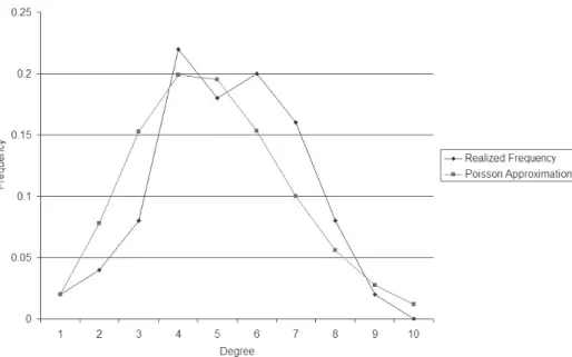
are common to this range of p and n. First, we should expect some isolated nodes. Based on the approximation of a Poisson distribution (1.4) withn= 50andp=:02, we should expect about 37.5 percent of the nodes to be isolated (i.e., have d= 0), which is roughly 18 or 19 nodes. There are 19 isolated nodes in the network, by chance. Figure 1.5 compares the realized frequency distribution of degrees with the Poisson approximation.
15The networks in Figures 1.4 and 1.6 were generated and drawn using the random network generator
The distributions match fairly closely. The network also has some other features that are common to random networks withp’s andn’s in this relative range. In graph theoretical terms, the network is a “forest,” or a collection of trees. That is, there are no cycles in the network (where a cycle is a sequence of links that lead from one node back to itself, as described in more detail in Section 2.1.3). The chance of there being a cycle is relatively low with such a small link probability. In addition, there are six components (maximal subnetworks such that every pair of nodes in the subnetwork is connected by a path or sequence of links) that involve more than one node. And one of the components is much larger than the others: involving 16 nodes, while the next largest component only has 5 nodes in it. As we shall discuss shortly, this is to be expected.
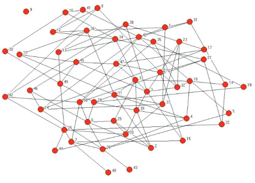
Next, let us start with the same number of nodes, but increase the probability of a link forming to p = log(50)=50 = :078, which is roughly the threshold where isolated nodes should start to disappear. (This threshold is discussed in more detail in Chapter 4.) Indeed, based on the approximation of a Poisson distribution (1.4) with n = 50
andp=:08, we should expect about 2 percent of the nodes to be isolated (with degree 0), or roughly 1 node out of 50. This is exactly what we see in the realized network in Figure 1.6 (again, by chance). With the exception of the single isolated node, the rest of the network is connected into one component.
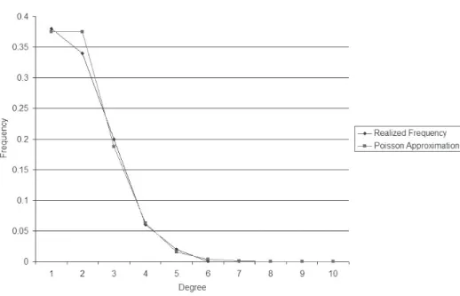
As shown in Figure 1.7, the realized frequency distribution of degrees is again similar to the Poisson approximation, although, as one should expect at this level of randomness, not a perfect match.
The degree distribution tells us a great deal about a network’s structure. Let us examine this in more detail, as it provides a …rst illustration of the concept of a phase transition, where the structure of a random network changes as we change the formation process.
Consider what fraction of nodes are completely isolated; i.e., what fraction of nodes have degree d = 0? From (1.4) it follows that this is approximated by e (n 1)p for
large networks, provided the average degree (n 1)p is not too large. To get a more precise expression, let us examine the threshold where this fraction is just such that we expect to have one isolated node on average. That is where e (n 1)p = 1
n. Solving
this yields p(n 1) = log(n), or right at the point where average degree (n 1)p is
Figure 1.6: A Randomly Generated Network with Probability .08 of each Link
4.2.2. If the average degree is substantially above log(n), then probability of having any isolated nodes goes to 0, while if the average degree is substantially below log(n), then the probability of having at least some isolated nodes goes to 1. In fact, as we shall see in Theorem 4.2.1, this is the threshold such that if the average degree is signi…cantly above this level then the network is path-connected with a probability converging to 1 asngrows (so that any node can be reached from any other via a path in the network), while below this level the network will consist of multiple components with a probability going to 1.
t t t
+ 2+ 3 c 2 + 2 2c
1 2 3 4
2 + 2 2c + 2+ 3 c
Figure 1.8: The utilities to the players in a three-link four-player network in the sym-metric connections model.
1.2.4
The Symmetric Connections Model
Although random network formation models give us some insight into the sorts of characteristics that networks might have, and exhibit some of the features that we see in the Add Health social network data, it does not provide as much insight into the Florentine marriage network. There, marriages were carefully arranged. The last example comes from the game-theoretic, economics literature and provides a basis for the analysis of networks that are formed when links are chosen by the agents in the network. Through this example, we can begin to look at the questions about which networks might be best for a society and which networks might arise if the players have discretion in choosing their links.
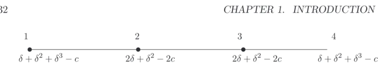
It is a simple model of social connections that was developed by Jackson and Wolin-sky [345]. In this model, links represent social relationships, for instance friendships, between players. These relationships o¤er bene…ts in terms of favors, information, etc., and also involve some costs. Moreover, players also bene…t from indirect relationships. A “friend of a friend” also results in some indirect bene…ts, although of a lesser value than the direct bene…ts that come from a “friend.” The same is true of “friends of a friend of a friend,” and so forth. The bene…t deteriorates with the “distance” of the relationship. This is represented by a factor that lies between 0 and 1, which indicates the bene…t from a direct relationship and is raised to higher powers for more distant relationships. For instance, in the network where player 1 is linked to 2, 2 is linked to 3, and 3 is linked to 4: player 1 gets a bene…t of from the direct connection with player 2, an indirect bene…t of 2 from the indirect connection with player 3, and an indirect bene…t of 3 from the indirect connection with player 4. The payo¤s to this four players in a three-link network is pictured in Figure 1.8.
For < 1 this leads to a lower bene…t from an indirect connection than a direct one. Players only pay costs, however, for maintaining their direct relationships.16
16In the most general version of the connections model the bene…ts and costs may be relation
Given a network g,17 the net utility or payo¤ u
i(g) that player i receives from a
network g is the sum of bene…ts that the player gets for his or her direct and indirect connections to other players less the cost of maintaining his or her links. In particular, it is
ui(g) =
X
j6=i: i and j are path connected in g
`ij(g) d
i(g)c;
where `ij(g) is the number of links in the shortest path between i and j, di(g) is the
number of links thatihas (i’s degree), andc > 0is the cost for a player of maintaining a link.
The highly stylized nature of the connections model allows us to begin to answer questions regarding which networks are “best” (most “e¢cient”) from society’s point of view, as well as which networks are likely to form when self-interested players choose their own links.
Let us de…ne a network to bee¢cientif it maximizes the total utility to all players in the society. That is, g is e¢cient if it maximizes Piui(g).18
It is clear that if costs are very low, it will be e¢cient to include all links in the network. In particular, if c < 2, then adding a link between any two agents i
andj will always increase total welfare. This follows because they are each getting at most 2 of value from having any sort of indirect connection between them, and since 2 < c, the extra value of a direct connection between them increases their utilities (and might also increase, and cannot decrease, the utilities of other agents).
When the cost rises above this level, so that c > 2 but c is not too high (see Exercise 1.3), it turns out that the unique e¢cient network structure is to have all players arranged in a “star” network. That is, there should be some central player who is connected to each other player, so that one player hasn 1links and each of the other players has 1 link. The idea behind why a star among all players is the unique e¢cient structure in this middle cost range, is as follows. A star involves the minimum number of links needed to ensure that all pairs of players are path connected, and it has each player within two links of every other player. The intuition behind this dominating
to some geography, so that linking with a given player depends on their physical proximity. That variation has been studied by Johnson and Gilles [351] and is discussed in Exercise 6.13.
17For complete de…nitions, see Chapter 2. For now, all that is important is that this tells us which
pairs of players are linked.
18This is just one of many possible measures of e¢ciency and societal welfare, which is a
1 4 2 3 t t t t
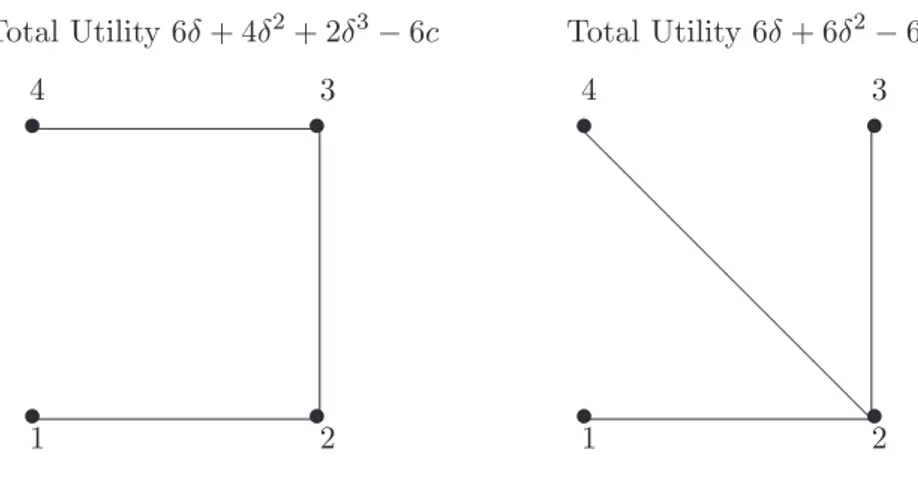
Total Utility 6 + 4 2+ 2 3 6c Total Utility 6 + 6 2 6c
1 4 2 3 @ @ @ @ @ @ @ @ @ @ t t t t
Figure 1.9: The Gain in Total Utility from Changing a “Line” into a “Star”.
other structures is then easy to see. Suppose for instance we have a network with links between 1 and 2, 2 and 3, and 3 and 4. If we change the link between 3 and 4 to be one between 2 and 4, we end up with a star network. The star network has the same number of links as our starting network, and thus the same cost and payo¤s from direct connections. However, now all agents are within two links of each other whereas before some of the indirect connections involved paths of length three. This is pictured in Figure 1.9.
As we shall see, this is the key to the set of e¢cient networks having a remarkably simple characterization: either costs are so low that it makes sense to add links, and then it makes sense to add all links, or costs are so high that no links make sense, or costs are in a middle range and the unique e¢cient architecture is a star network. This characterization of e¢cient networks being either stars, empty or complete, actually holds for a fairly general class of models where utilities depend on path length and decay with distance, as is shown in detail in Section 6.3.
relationship that he or she is involved in, then that link would be deleted; while if two individuals would each bene…t by forming a new relationship, then that link would be added.
In the case where costs are very lowc < 2, as we have already argued, the direct bene…t to the agents from adding or maintaining a link is positive, even if they are already indirectly connected. Thus, in that case the unique pairwise stable network will be the e¢cient one which is the complete network. The more interesting case comes when c > 2, but c is not too high, so that the star is the e¢cient network. If > c > 2, then a star network (that involves all agents) will be both pairwise stable and e¢cient. To see this we need only check that no player wants to delete a link, and no two agents both want to add a link. The marginal bene…t to the center player from any given link already in the network is c >0, and the marginal bene…t to a peripheral player is + (n 2) 2 c >0. Thus, neither player wants to delete a link. Adding a link between two peripheral players only shortens the distance between them from two links to one, and does not shorten any other paths - and sincec > 2
adding such a link would not bene…t either of the players. While the star is pairwise stable, in this cost range so are some other networks. For example if c < 3, then four players connected in a “circle” would also be pairwise stable. In fact, as we shall see in Section 6.3, many other (ine¢cient) networks can be pairwise stable.
If c > , then the e¢cient (star) network will not be pairwise stable, as the center player gets only a marginal bene…t of c <0from any of the links. This tells us that in this cost range there cannot exist any pairwise stable networks where there is some player who just has one link, as the other player involved in that link would bene…t by severing it. For various values of c > there will exist nonempty pairwise stable networks, but they will not be star networks: as just argued, they must be such that each player has at least two links.
This model makes it clear that there will be situations where individual incentives are not aligned with overall societal bene…ts. While this connections model is highly stylized, it still captures some basic insights about the payo¤s from networked relation-ships and it shows that we can model the incentives that underlie network formation and see when resulting networks are e¢cient.
endogenous to the network formation process (as is true in many market and partner-ship applications)? Uow does the relationpartner-ship between the e¢cient networks and those which form based on individual incentives depend on the underlying application and payo¤ structure?
1.3
Exercises
Exercise 1.1 A Weighted Betweenness Measure
Consider the following variation on the betweenness measure in (1.1). Any given shortest path between two families is weighted by inverse of the number of intermediate nodes on that path. For instance, the shortest path between the Ridol… and Albizzi involves two links and the Medici are the only family that lies between them on that path. In contrast, between the Ridol… and the Ginori the shortest path is three links and there are two families, the Medici and Albizzi, that lie between the Ridol… and Ginori on that path.
More speci…cally, let `ij be the length of the shortest path between nodes i andj
and let Wk(ij) =Pk(ij)=(`ij 1), (setting `ij = 1 and Wk(ij) = 0 if i and j are not
connected). Then the weighted betweenness measure for a given node k be de…ned by
W Bk =
X
ij:i6=j;k =2fi;jg
Wk(ij)=P(ij)
(n 1)(n 2)=2: (1.5)
where we take the convention that Wk(ij)
P(ij) = 0=0 = 0 if there are no paths connecting i andj.
Show that
W Bk > 0 if and only if k has more than one link in a network and some of k’s
neighbors are not linked to each other,
W Bk = 1 for the center node in a star network that includes all nodes (with
n 3), and
W Bk < 1unlessk is the center node in a star network that contains all nodes.
Calculate this measure for the the network pictured in Figure 1.10 for nodes 4 and 5.
Figure 1.10: Di¤erences in Betweenness measures.
Exercise 1.2 Random networks
Fix the probability of any given link forming in a Poisson random network to bep
where1> p >0. Fix some arbitrary network g on k nodes. Now, consider a sequence of random networks indexed by the number of nodes n, as n ! 1. Show that the probability that a copy of thek node networkgis a subnetwork of the random network on then nodes goes to 1 as ngoes to in…nity.
[Hint: partition the n nodes into as many separate groups of k nodes as possible (with some leftover nodes) and consider the subnetworks that end up forming on each of these groups. Using the expression in (1.2) and the independence of link formation, show that the probability that the none of these match the desired network goes to 0 as n grows.]
Exercise 1.3 The Upper Bound for a Star to be E¢cient
Exercise 1.4 The Connections Model with Low Decay
Consider the symmetric connections model in a setting where1> > c >0. Show that if is close enough to 1, so that there is “low decay” and n 1 is nearly , then in every pairwise stable network every pair of players have some path between them and that there are at mostn 1total links in the network.
In a case where is close enough to 1 so that any network that hasn 1links and connects all agents is pairwise stable, what fraction of the pairwise stable networks are also e¢cient networks?
How does that fraction behave as n grows (adjusting to be high enough as n
grows)?
Exercise 1.5 Homophily and Balance Across Groups
Consider a society of two groups, where the set N1 comprises the members of group 1 and the set N2 comprises the members of group 2, with cardinalities n1 and
n2, respectively. Suppose that n1 > n2. For an individual i, let di bei’s degree (total
number of friends) and letsidenote the number of friends thatihas that are within own
group. Let hk denote a simple homophily index for groupk, de…ned byhk =
P
i2Nksi
P
i2Nkdi.
![Figure 1.1: 15th Century Florentine Marriges Data from Padgett and Ansell [493]](https://thumb-eu.123doks.com/thumbv2/123dok_br/16390964.725076/3.892.135.710.203.546/figure-th-century-florentine-marriges-data-padgett-ansell.webp)
![Figure 1.2: A Figure from Bearman, Moody and Stovel [47] based the Add Health Data Set](https://thumb-eu.123doks.com/thumbv2/123dok_br/16390964.725076/6.892.212.678.299.627/figure-figure-bearman-moody-stovel-based-health-data.webp)