A Work Project, presented as part of the requirements for the Award of a Masters Degree in Finance from the NOVA - School of Business and Economics
AN EQUITY WEALTH PRESERVATION STRATEGY:
FOLLOWING THE MACRO TREND
GUILHERME GOMES PESTANA FERREIRA DE ALMEIDA – 880
A Project carried out on the Financial Markets major under the supervision of:
Professor Martijn Boons
AN EQUITY WEALTH PRESERVATION STRATEGY:
FOLLOWING THE MACRO TREND
Abstract
Financial crisis have happened in the past and will continue to do so in the future. In the most recent 2008 crisis, global equities (as measured by the MSCI ACWI index) lost a staggering 54.2% in USD, on the year. During those periods wealth preservation becomes at the top of most investor’s concerns. The purpose of this paper is to develop a strategy that protects the investment during bear markets and significant market corrections, generates capital appreciation, and that can support Millennium BCP’s Wealth Management Unit on their asset allocation procedures. This strategy extends the Dual Momentum approach introduced by Gary Antonacci (2014) in two ways. First, the investable set of securities in the equities space increases from two to four. Besides the US it will comprise the Japanese, European (excl. UK) and EM equity indices. Secondly, it adds a volatility filter as well as three indicators related to the business cycle and the state of the economy, which are relevant to decide on the strategy’s exposure to equities. Overall the results attest the resiliency of the strategy before, during and after historical financial crashes, as it drastically reduces the downside exposure and consistently outperforms the benchmark index by providing higher mean returns with lower variance.
I. Introduction
This paper aims to produce an equity strategy that simultaneously seeks capital preservation by avoiding significant market disruptions and generates long-term capital appreciation, outperforming the global equity index. It also intends to fulfil Millennium BCP’s Wealth Management Unit (WMU) needs for a quantitative and straight-forward model to assess the overall state of the equity markets and decide on the exposure of the clients’ portfolios to this asset class across geographies on a monthly basis1. Hence, the practicality of the strategy constructed was prioritized over complex and time-consuming methods.
The approach followed in this study expands that of the dual momentum model introduced by Gary Antonacci (2014). In his book, the investment portfolio switches between US stocks, non-US stocks and short-to-intermediate term bonds. The portfolio is either invested in non-US stocks or non-US stocks in accordance to relative momentum, and will hold bonds when equities are not in an uptrend, as determined by the absolute momentum rule.
As to the strategy introduced by this paper, the investment portfolio will move across US, European (excl. UK), Japanese and Emerging Market economies stocks according to the relative momentum component. The decision to hold an alternative debt security however, will not only depend on the existence of absolute momentum. Rather other indicators come into play, namely the realized volatility of the US stock market returns, the evolution of the trailing earnings per share linked to the US companies and the 10-year and the 3-month US Treasury yields. It will switch back and forth from equities depending on the signal produced by the majority of the indicators. If they suggest investing in equities, relative momentum selects the stronger equity
1
This work project has a directed research internship format (DRI), and was complemented by other assignments designed to provide a solid on-the-job training at Millennium BCP’s WMU. Millennium BCP is the largest privately owned bank in Portugal and currently run operations in Poland, Mozambique, Angola and Switzerland. The WMU is part of the Private Banking Division and has five main responsibilities: manage the portfolios on behalf of its private and institutional customers; analyze and monitor the financial markets; select investment funds; design structured products; provide advisory services. The WMU’s organogram is presented in the appendix (Figure 1).
index from the basket of four indices. The additional components included in this model are expected to help signaling a future deceleration of economic activity and to provide information that may not be captured by momentum. Whenever the current or future performance of equities is perceived as weak, the investment will be temporarily allocated in bonds until the equity markets recover. The fact that most of the time the strategy is fully invested in equities avoids the drag in real returns that a permanent bond allocation imposes over the long-run, due to inflation. This approach leads to a substantial outperformance relative to the benchmark defined by the MSCI ACWI index, while achieving a better risk-reward profile and reducing the overall drawdown relative to the dual momentum strategy. The Sharpe ratio improves from 0.85 for dual momentum to 0.97, and the Information ratio increases from 2.00 to 2.35. As to the maximum drawdown, it is -23.0% for dual momentum and -15.8% for the strategy, which is substantially lower than the 54.2% drawdown for the benchmark index. Compared to dual momentum, our results suggest the task of timing the market is more effective when additional information about the business cycle is taken into account, since our strategy captures more of the returns when global equities are up, and reduces downside exposure when stock returns are negative.
The transactions costs, they should be minimal given the strategy can be performed using ETFs, and because the portfolio is rebalanced less than four times a year, on average. The strategy presented in this paper compares most favorably to a buy-and-hold approach over a long-term investment horizon. Even though on a short-long-term basis, there is a potential for whipsaw losses due to false signals, the attractive risk-reward of the strategy and its significant outperformance during both up and down market environments brings confidence that the long-term net effect of avoiding emotionally based decisions is very positive. In the end, there are always going to be trade-offs and there is no strategy that guarantees an investor exits the stock market right at the top, nor get in right at the bottom.
The rest of the document is organized as follows. The next section presents the literature review. The data are discussed in Section III, while Section IV explains in detail each component of the model and develops alternative strategies that aggregate the different individual components. In Section V the key results are presented and discussed. Section VI concludes.
II. Literature Review
A. The Momentum Anomaly
Momentum is one of the most persistent and puzzling anomalies in the financial markets. The basic idea of trend following is an old concept, and goes back to as far as the 19th century, being attributed to David Ricardo the famous saying: “Cut short your losses, let your profits run”.
Literature on this topic has been steadily increasing since Jegadeesh and Titman (1993) result that buying winners and selling losers based on their past performance produces returns in excess to those of the market. A considerable number of studies show momentum exists within and across various asset classes and geographies and is robust with respect to time.
Although until today there is no consensus on what causes momentum and its abnormal profits, we can identify two distinct schools of thought. First there is the risk-based explanation, consistent with the idea of rational efficient markets, which assumes momentum profits are a compensation for bearing its risk. However, Jegadeesh and Titman (2001) argue against the hypothesis that momentum profitability is generated from cross-sectional variations in expected returns of individual stocks, and Grundy and Martin (2001) suggest that expected returns from time-varying risk factors also fail to explain momentum profitability. Several studies continued to
search for additional risk factors and construct risk-based models2, regardless of the risks of data mining and experiencing overfitting bias. The second type of explanations emanates from the behavioral finance field, which sees momentum profits not as a compensation for risk but rather irrationality and systematic biases displayed by investors. DeLong et al. (1990) suggest that when traders follow positive-feedback strategies, meaning they buy (sell) securities when prices rise (fall), prices tend to overreact and generate momentum. Subsequent studies have proceeded to debate the role of behavioral biases in causing momentum.3
One way or another, researchers recognize that momentum has persisted throughout time and in different asset classes. Fama and French (2008) called momentum “the center stage anomaly”.
It is important for the purpose of this paper to distinguish between two types of momentum. The first type is defined as relative momentum, also called cross-sectional momentum, which compares the past performance of different assets and then separates “winners” from “losers”. Strategies that exploit relative momentum are often tested on a market-neutral basis by simultaneously buying winners and selling short losers. Asness, Liew, and Stevens (1997) find momentum helps to explain the cross-section of expected country stock index returns and Bhojraj and Swaminathan (2006) provide evidence that winners outperform losers on the context of international stock market indices.
The second type is absolute momentum (also termed time-series momentum), and focuses on a security’s own performance over a given look-back period. Moskowitz, Ooi, and Pedersen (2012) show that absolute momentum profits are robust across different asset classes and markets, and are larger when stock market returns are the most extreme. Furthermore, Hurst, Ooi and Pedersen
2 Chordia and Shivakumar (2002) include lagged macroeconomic variables related to the business cycle. Liu and
Zhang (2008) apply the growth rate of industrial production.
3 Barberis, Shleifer, and Vishny (1998) argue that investors initially underreact to news due to conservatism and
subsequently overreact over longer periods due to representativeness. Daniel, Hirshleifer, and Subrahmanyam (1998) suggest investors are subject to overconfidence.
(2012) show absolute momentum is just as robust and universal as relative momentum, arguing that it has been profitable since 1903 and across 59 markets including in country stock indices.
Gary Antonacci (2014) when comparing absolute and relative momentum says the following: “It is possible for an asset to display positive relative momentum if it is strong relative its peers and to have negative absolute momentum if its own trend has been down. It can also have positive absolute momentum if its trend has been positive and negative relative momentum if another asset has been going up more”. He shows that by using them together investors can benefit from the higher risk-premium of equities, while reducing volatility and the likelihood of large drawdowns by holding bonds when the upward trend in equities is weakening. In his book, he looks at an investment portfolio composed by US stocks (S&P500 Index), non-US stocks (MSCI ACWI ex-US) and an US bond index (Barclays US Aggregate Bond Index). First, Antonacci uses relative momentum to select the best-performing asset between US and non-US stocks over the preceding year. After identifying which asset displays the stronger trend, he compares the excess returns of the selected index over the T-bill rate in the previous 12-month period to determine if the absolute momentum is positive or negative. If it has been positive, that means the strategy will invest in best performing stock index on a relative basis. If absolute momentum is negative, then the strategy‘s investment will move to the bond instrument (the Barclays US Aggregate Bond Index) until the trend in equities turns positive again. During bear markets bonds will serve as a safe harbor, while in bull markets the strategy is in harmony with the trend of the stock market. Antonacci’s dual momentum strategy doubles the annual rate of return over the MSCI ACWI, reduces volatility by 200bps, and achieves a 0.87 Sharpe ratio, from 1974 until 2013. Moreover, the combination of both momentum components results in a major outperformance during down market environments, averaging a +2.2% annual return during S&P500 bear years and lowering the maximum drawdown by nearly two-thirds.
While previous literature has focused predominantly on relative momentum, its applicability is challenging as it encompasses a very high exposure to risk and do not protect investors against extreme losses. Gary Antonacci (2014) argues that although relative momentum boosts annual returns in up market environments, it offers no advantage over the market when the trend in equities is collapsing, and helps little to reduce volatility and downside exposure. Daniel and Moskowitz (2012) find that the distribution of returns associated to relative strength strategies has a very pronounced left tail, suggesting that if a crash occurs it can erode returns substantially. Santa-Clara and Barroso (2012) show that the strategy of buying past winners and selling past losers in the US stock market would have delivered extremely negative (cumulative) returns during very short periods of time in 1932 (-91.59%) and 2009 (-73.42%). To solve this, they construct a “risk-managed momentum” strategy that after incorporating a volatility target, practically avoids crash risk (reduces kurtosis and left skew), lowers standard deviation, and enhances returns compared to the original relative momentum approach.
This paper develops a strategy that combines the two types of momentum, being greatly inspired by the powerful evidence presented by Gary Antonacci (2014), and adds a volatility component applied at the aggregate stock market to limit the occurrence of large drawdowns.
B. Equity returns and the Business Cycle
The exact relationship between macroeconomic shocks and the stock market remains unclear today. McQueen and Roley (1993), for instance, suggest stock prices react differently to the release of economic indicators depending on the actual stage of the business cycle. Li and Hu (1998) validate this hypothesis but show that the impact of many macroeconomic announcements on stock prices varies depending on how they proceed to classify the actual economic state. Their study demonstrates how difficult it has been to provide significant and reliable conclusions
regarding the influence of fundamental information about the economy on stock prices. The lack of solid empirical evidence increases the probability that investors misinterpret or overlook the general market sentiment about macroeconomic news, and make poor investment decisions.
This perhaps partially explains why academics have focused on other proxies for the business cycle when trying to estimate future stock returns. In particular, earlier work has investigated the impact of interest rates and corporate earnings on equity returns.
Starting by short-term interest rates, they are relevant because short-term bonds are frequently seen as an alternative close to a safe investment relative to equities. In addition, short-term rates serve as proxy for the rates used to discount future profits, at least in the short-run. A negative correlation between short-term interest rates and future stock market returns is documented by Fama and Schwert (1977). They also show that this variable serves as a proxy for expectations of future economic activity. This interpretation is consistent with that of Breen, Glosten, and Jagannathan (1989) who attribute the forecasting ability of short-term interest rates over stock returns to its economic significance. More recently, Bordo and Wheelock (2006) argue that past stock market booms typically have arisen when short-term rates were low and/or falling, and have ended with tighter monetary policy conditions reflected in increasing interest rates.
Past literature also covered the relationship between the yield spread and equity returns. The yield spread is the difference between a long-term interest rate (e.g. 10-year Treasury bond) and a short-term interest rate (e.g. 3-month Treasury bill). Fama and French (1989) document the predictive power of the yield spread to forecast excess stock returns and show that this variable is closely related to short-term business cycles. The same authors (Fama and French (1993)) include the yield spread to explain stocks and bond returns using common risk factors.
Although the yield spread is in essence a financial variable, it is widely understood as a leading economic indicator because it reflects the stance of the monetary policy which in turn
impacts future economic activity. In a scenario where monetary policy tightens, short-term interest rates in principle increase more than long-term interest rates. If the movement is strong enough long-term rates may display a lower yield than short-term rates, a phenomenon called inverted yield curve. This is perceived as signaling the end of the expansionary stage of the economic cycle, because in general a more restrictive monetary policy reduces spending and investment, causes economic growth to slow down and increases the probability of a recession. This is especially relevant because according to Conover, Jensen, and Johnson (1999) equity returns are considerably higher during periods of expansionary monetary policy and much lower when monetary policy is more restrictive.
Lastly, despite many studies have avoided the use of earnings data mainly due to complicated and time-changing accounting procedures and definitions, corporate earnings continue to be a convenient measure for investors to evaluate the fundamental value of companies and predict future cash-flows. At the aggregate level, because earnings growth proxies for corporate profits growth, it conveys information about the economy given corporate profits is a component of GDP. Regarding this, Konchitchki and Patatoukas (2014) argue that aggregate accounting earnings growth is a leading indicator of the US economy.
Yet the link between stock returns and earnings is more controversial. In 1968, Ball and Brown documented a positive association between stock returns and earnings growth at the individual firm level. Contrary to existing evidence at the firm level, Kothari, Lewellen, and Warner (2006) show that in the US, aggregate stock market returns are negatively related with aggregate earnings changes. They attribute this to a positive association between earnings and interest rates, and thus discount rates. However, He and Hu (2014) argue that US is an unique phenomenon and find a positive association between stock market returns and aggregate earnings growth in international markets.
Overall we expect these macro-related indicators to help signal a future deceleration of economic activity that eventually may drag down stock market performance. By providing additional information which may not be captured by momentum, we anticipate the investor will be warned on a timely manner when there is a latent bear equity market ahead.
III. Data
Monthly data for the stock indices was collected from Bloomberg covering the period from 1990 to 2015. The individual series on the MSCI ACWI, MSCI USA, MSCI Europe excl. UK, and MSCI Emerging Markets are total returns gross of dividends measured in US dollars. The MSCI indices are composed by the largest and the most liquid stocks and those which have most information available to investors.
The choice of the MSCI ACWI index as the benchmark for a global equity strategy replicates the procedures from Millennium BCP WMU when evaluating the relative performance of their portfolio on the equities space. Moreover, in this paper we restrict the investable set of equity indices to the US, Europe (excluding UK), Japan, and Emerging Markets because the strategy should reproduce the most likely exposures that the portfolio of a given client may face depending on the general asset allocation decisions.
The historical monthly data from 1990 until 2015 on the one-month US T-bill rate was retrieved from Kenneth French’s online library. This paper will also present the results obtained when the strategy replaces the one-month T-bill by an US bond index to determine absolute momentum and to serve as the safe investment alternative to equities. This index will be the Barclays U.S. Aggregate Bond Index which historically has been stable in terms of composition, selecting high-quality, investment grade bonds with an average maturity under five years. The respective monthly total return series measured in US dollars was retrieved from Bloomberg.
Monthly data on the yields associated to the ten-year US Treasury bond and the three-month US Treasury bill was also retrieved from Bloomberg. In this paper, the yield spread is defined by the difference between those two yields.
The 12-month trailing earnings per share (EPS) series from the MSCI USA index was gathered from Datastream and comprises monthly data from January 1990 to February 2015. Trailing EPS are preferred over a similar forward looking measure because the strategy is designed to include only past information. This way, the power of the signal to be included in the strategy will not be mistaken by the superior forecast accuracy from analysts regarding earnings growth and captures information only about actual data. Moreover, although it is true that changes in aggregate EPS are not directly translated into changes in aggregate earnings because of the dilution effect associated to capital increases that weigh down EPS growth, the strategy’s key priority is to identify the future direction of the business cycle which ultimately should be validated by the trend in profits.
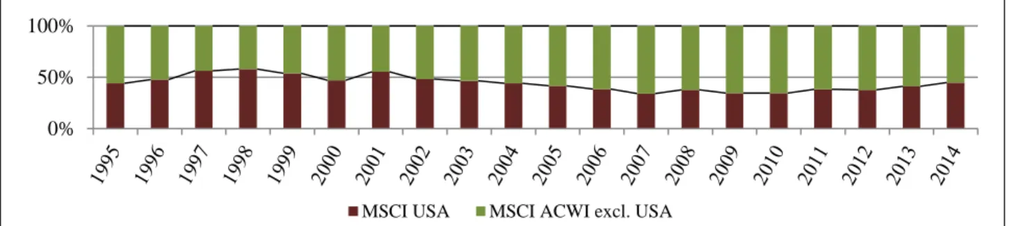
One relevant topic is our emphasis on variables linked to the US. Currently, the US economy remains the largest economy in the world and exerts huge influence on several other open economies. Through bilateral trade we expect shocks on the US economy to have some impact on other developed and developing countries. Moreover, we observe that the US economic supremacy finds a parallel in financial markets. Figure 2 shows US equities have been by far dominating the global equity market in market-cap terms. The weight that the MSCI ACWI index, which is a well-known and accepted gauge of global stock market performance, attributes to US stocks (approximately 53% as at September 2015) also illustrates this idea. On top of this, Rapach, Strauss, and Zhou (2013) argue that returns in the US stock market lead those in non-US equity markets.
IV. Strategy Construction
The following section starts by explaining the two momentum components. Then it proceeds to describe the additional indicators to be included in the model, and ends up explaining how the different strategies were built and in what way they should be implemented.
A. Momentum Components
This paper exploits the momentum anomaly by using the dual momentum approach introduced by Gary Antonacci (2014) who combines absolute with relative momentum.
Both components do essentially the same thing, which is to identify price strength that is likely to persist. The relative momentum component is built after comparing the average return in the past twelve months of the MSCI stock indices the strategy is able to invest in: USA, Europe excluding UK, Japan and EM. The equity index with the stronger performance over the previous year is said to display relative momentum. Absolute momentum is determined by comparing the last twelve-month average returns of the MSCI USA to those of an alternative safe asset. The MSCI USA index is in an uptrend if the excess return in the preceding year was positive.
We use momentum as a technical trading rule in accordance to the findings of Zakamulin (2015), who shows that momentum gives better results than moving average rules regardless of the length of the investment horizon. The formation (or look-back) period for momentum will be 12 months, which is in agreement with past literature on this topic4. When dealing with individual stocks, most studies suggest skipping one month between the formation period and the implementation of the momentum strategy due to a short-term reversal effect attributed to liquidity or microstructure issues. By incorporating ETFs that track the performance of stock indices, however, this issue is less relevant, and thus that procedure is not taken into account.
B. Additional Components
A volatility indicator is constructed based on the standard deviation of the last 12-month returns of the MSCI USA index. We choose an annualized volatility target of 10%. This is below the annualized volatility target of 12% picked by Santa-Clara and Barroso (2012) in the strategy they called “risk-managed momentum”, and also stands below the annualized volatilities of returns of the MSCI ACWI index (15.6%) and the popular size (11.4%), value (10.8%) and momentum (17.4%) factors from January 1990 to September 2015. 5
Therefore, a 10% target seems reasonable from an investor standpoint, and is in line with a key element of the strategy that is to preserve capital and avoid significant downside exposure. Moreover, this component is also expected to balance the risks incurred by momentum, based on the evidence presented by Tang and Mu (2012) that momentum profits are negatively related to volatility. The rule associated to this indicator is the following: If the variability of the returns of the MSCI USA index over the past year, as measured by the annualized standard deviation, is higher than 10%, the strategy should not invest in equities in the current month and exit to the safety of the alternative debt security; otherwise it generates a buy signal towards equities.
Two indicators related to the US interest rates are also considered. The first is linked to the US yield curve. When the yield curve inverts, meaning the yield on the short-term 3-month Treasury bill rises above the yield on the long-term 10-year Treasury bond, the strategy receives a signal to exit out of equities in the following month and seek safety in the alternative safe security. This is because an inverted yield curve generally reflects that investors are expecting short-term interest rates to fall in the future, reacting to monetary policy loosening by the Fed to counter a potential economic slowdown. This in turn feeds investors willingness to hold long-term bonds, pushing
long-term yields down. Providing the yield spread is positive, expectations for a recession over the near term are low. This implies the indicator favors equity exposure.
The second indicator is only linked to the 3-month T-bill yield, and tracks its past two year’s performance as well as the direction of its monthly changes. If the yield on the previous month is lower than the two-year moving average and at the same time it has decreased from the preceding month, then a signal to invest in equities in the current month is delivered. If one or both conditions are not met, meaning that the 3-month yield is quoting higher than the historical two-year average and/or it has increased over the previous month, the strategy is advised to exit equities and seek protection in the alternative debt security.
The fourth and final additional indicator to be included in the strategy refers to corporate earnings. Earnings provide information about current and expected future profitability and from the equity holders standpoint it conveys data of current and expected future dividends, which in theory are directly related to stock prices. Assuming the discount rate is unchanged, earnings growth suggest an increase in cash-flows which in principle does lead to higher stock prices. However, and as mentioned before, recent literature has suggested that aggregate earnings are negatively related to US stock market returns, due to an increase in discount rates that dominates the positive effect from cash-flows. As the discount rate effect is already included in the strategy through the interest rates components, the role for the earnings indicator will be to inform about the evolution in cash-flows and hint about the current stage of the business cycle from the firms’ standpoint. This paper uses the MSCI USA 12-month trailing EPS to evaluate the overall earnings trend in the US stock market. The indicator will give a buy signal towards equities on the current month if the yearly change of the 12-month trailing EPS recorded on the previous month was positive and the previous month value is higher than the 1-year average. Meaning the
strategy will invest in equities if earnings have been increasing and are at relatively high levels. Otherwise, the indicator hints to move away from equities.
C. Different Strategies’ Specifications
Momentum is a central bloc of the strategies developed in this paper. As such, the first three strategies constructed are based on absolute momentum, relative momentum and a combination of both (Dual Momentum strategy).
A strategy that looks exclusively at absolute momentum will be applied as following. If the MSCI USA shows a positive excess return (return less that of the alternative safe asset) during the past 12 months, the strategy invests in a portfolio composed by the MSCI indices covering US, European excluding UK, Japanese and EM stocks. The weight of each stock market index is fixed and remains unchanged throughout the investment period. As presented in Table 1, these indices will have the same relative weights as in the MSCI ACWI, which serves as the benchmark for all strategies. If the prior 12-month excess return of the MSCI USA is negative, the strategy exits the equity index it was invested in and holds the safe asset instead. It will reinvest in equities when the MSCI USA excess return is again positive.
The relative momentum strategy implies we will switch the portfolio across the MSCI indices based on their relative performance on the previous year. Each month, it will select the index that has displayed the highest returns in the preceding 12 months, even if all the stock markets are trending down. This happens because we do not diversify away from equities.
For a strategy that pools together the two types of momentum the first step is to compare the recent performances of the MSCI USA index to the alternative safe asset, applying the absolute momentum rule. If US stocks exhibit absolute momentum the strategy will invest in the equity index that has displayed the stronger performance in the last 12-months based on relative strength
momentum. If the 12-month excess return of the aggregate US stock market is negative, the strategy will exit its position in equities and hold the alternative safe investment.
This procedure is conducted every month. It is expected that dual momentum benefits from the particularities of both momentum components, and as a result it can improve the overall performance of the strategy against the benchmark index.
It is worth noting that the application of dual momentum described in Gary Antonacci book (2014) differs from the one presented in this paper in three ways. First, he applies the relative momentum rule to the index that over the preceding year has performed better. In other words, he first selects the strongest equity index based on the relative momentum rule, and then checks if this selected index has done better than the alternative debt security in accordance with the idea of absolute momentum. If it has, he invests in that index, if not he seeks protection by investing in the alternative debt security. This is in contrast to the procedure applied in this paper. On the one hand, our absolute momentum signals are taken from the comparison between the historical performance of the US stock market and the alternative safe harbor. On the other hand, we use absolute momentum as a first filter to define if an investor should or not invest in equities and only then (if the signal is positive) we proceed to examine which equity index has a performed better in the past 12 months. Finally, we select and invest in the best equity index among the options available. The third major modification is the following. Under Antonacci’s framework, an investor will look at the excess return of a given equity index over the US Treasury bills to define absolute momentum, but then will hold the Barclays US Aggregate Bond Index instead when that excess return is negative. In this paper, we examine two alternative versions. The first version is similar to Antonacci procedure in the sense the MSCI USA exhibits absolute momentum if it shows a positive excess return (return less the one month Treasury bill rate). However in this version, if the excess return is negative (i.e. no momentum in the US stock
market) the investor will invest in the one month Treasury bill. The second version follows the same procedure, but substitutes the Treasury bill by the Barclays Bond Index in both steps: 1) absolute momentum will now be conditional on the return of the MSCI USA Index in excess of the Barclays Bond Index, and 2) the investor will hold the Barclays Bond Index during a bear stock market in the US. In either case, the investor is able to diversify away from equities when market conditions are not favorable.
As to the next set of strategies, we combine momentum with other variables by extending the criteria used to decide when to invest or not in equities in a given month. If previously, a strategy would rely only on the absolute momentum rule to provide a buy (or sell) signal concerning a potential investment on a given equity index, now the decision also depends on the signals transmitted by the other indicators, using the rules defined above. Only when the majority of indicators are in favor of an equity investment should the strategies take on that position in the subsequent month. Figure 3 illustrates the logic behind a strategy that aggregates absolute momentum, relative momentum and the four additional indicators.
V. Results
The results of the aforementioned strategies are examined in this section. Each strategy has two versions depending on the alternative security that serves as the safe harbor from equities and to which the performance of the MSCI USA index is compared to (to check if absolute momentum exists). This will be either the one month Treasury bill or the Barclays US Aggregate Bond Index. Overall, it is expected the latter enhances returns while still providing a relatively safe place to park capital, thus making it more attractive from an investor’s perspective.
Table 2 summarizes the overall performance of the strategies associated to the Treasury bill (version 1) and Table 3 presents the same indicators for those same strategies that use the
Barcalys Index instead (version 2). The risk-adjusted performance is evaluated by three popular ratios: Sharpe ratio, Sortino ratio and Information ratio. Each one will produce a different result, depending on how they measure the risk that had to be taken to realize the profit. This procedure is intended to bring more transparency when comparing strategies and to analyze through different angles the robustness and consistency of each strategy. Nonetheless, they share a common principle: the higher the value of the ratio the better.
First, the performance of the absolute momentum strategy is evaluated. The benefits from employing this simple strategy become immediately clear. The average annual return increases by more than 300bps (+350bps in V1 and +430bps in V2) over the benchmark, while the annual standard deviation falls by more than 500bps (-570bps in V1 and -630bps in V2). Consequently, absolute momentum improves substantially risk-adjusted returns, all while still being invested in equities more than 90% of the time and demanding, on average, around one trade per year. The maximum drawdown is cut by a more than three-quarters, and the percentage of profitable months rises to around 70% from 61% in the case of the benchmark. It is also worth mentioning the performance of the absolute momentum strategy during down years for the MSCI ACWI. In 8 bear market years for global equities, absolute momentum outperforms the benchmark every year when considering version 1, and in 7 years according to version 2. During those 8 years the average annual return is -0.6% and +3.2%, respectively for versions 1 and 2, which compare to a return of -18% for the benchmark.
The performance of relative momentum differs greatly from absolute momentum. Overall, it improves the average annual return by 500bps in relation to the benchmark, but it comes with an increase of 430bps in volatility and a surge in the maximum drawdown from -54.2% to -62.3, which is recorded in 2008. Unlike absolute momentum, relative momentum boosts the yearly maximum return by 520bps to 35.5% in relation to the benchmark. Moreover, relative
momentum beats the benchmark in 15 out of 18 bull market years for global equities, achieving an average annual return of +23.1% versus +16.8% during up market environments.
Next, the performance of the dual momentum strategy is examined. The previous results show relative momentum alone has done little to reduce downside exposure during bear markets, despite boosting annual returns in up market environments. On the other hand, absolute momentum reduces volatility and downside exposure substantially and it serves as a buffer against negative events in the equities space. As expected dual momentum has a better risk-reward profile than the single absolute and relative momentum strategies. All three risk-adjusted performance measures improve, as the strategy achieves an annual average return of 14.2% and 14.8% with an annual volatility of 15.1% and 14%, respectively for V1 and V2. To implement this strategy an investor would have to make 2.2 (2.7) changes per year considering the version 1 (version 2), while spending above 70% of the months in equities. Dual momentum boosts the maximum annualized return to 43.1% achieved in 1999, surpassing a 30.3% return realized by the benchmark in 2009. The maximum drawdown in a year is virtually slashed by half comparing with the benchmark, and stands at -23%, which is higher than in the absolute momentum but considerably lower than the loss inflicted by the individual relative momentum strategy. From 1990 to 2015, dual momentum has provided a higher return in relation to the global equity market in 19 and 18 years, respectively under version 1 and version 2 frameworks. In 8 bear markets for the MSCI ACWI index dual momentum outperforms the benchmark in 6 and boosts considerably returns, highlighting one of its core features which is to keep capital relatively safe following severe market corrections and during protracted bear markets.
As shown in Table 2 and Table 3, by combining the dual momentum components with a few additional variables to decide when to entry or exit the equity markets, an investor could have also obtained interesting results and achieved a considerable outperformance over the benchmark
index. However, the strategy that brings together momentum, volatility, EPS and Treasury yields components (hereafter “Strategy All Variables”) stands out for two reasons. First, and unlike the two other strategies that are presented, it is invested in equities 70% of the time which is more in line with the goal of this paper, that is to construct an equity investment strategy. Second and more importantly, the strategy all variables perfects dual momentum in nearly all performance-related indicators, and therefore beats the benchmark by an even larger margin.
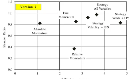
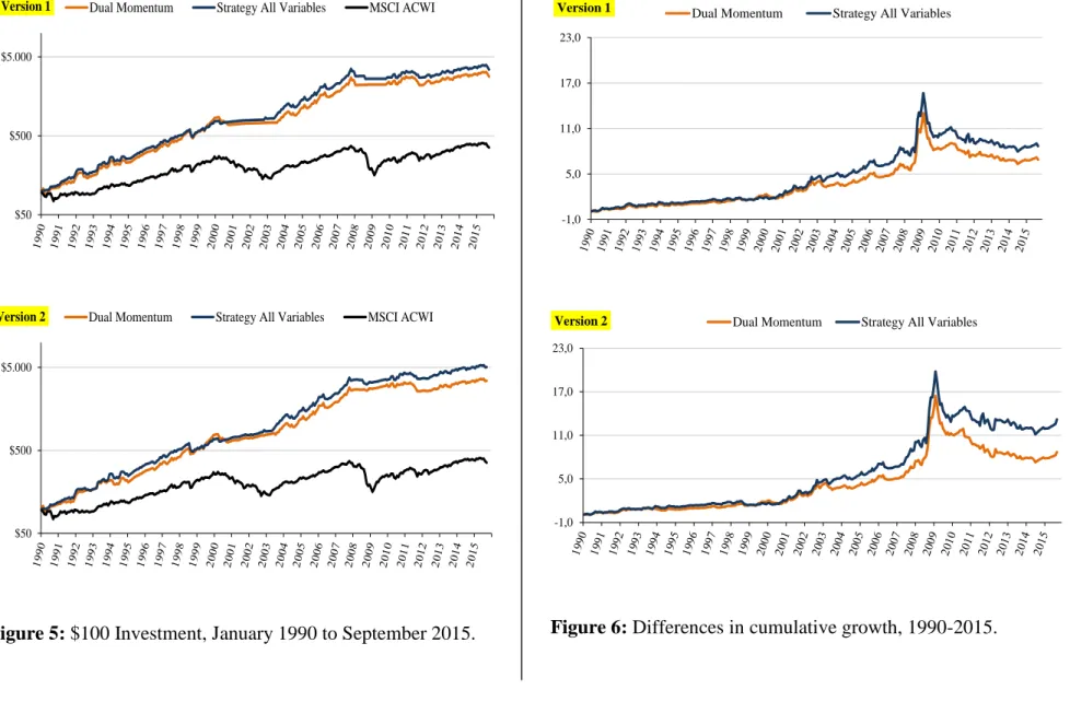
Figure 4 shows that this strategy produces a more attractive performance and has the best risk-reward profile, with approximately just one more switch per year on average in relation to dual momentum. This outperformance is corroborated by the Sortino and the Information ratios, in both versions. In dollar terms, if an investor had invested $100 in January 1990, he would have obtained $3450 ($5056) if he had performed the strategy all variables, $2822 ($3454) if he had opted by the dual momentum approach and only $356 if instead he had simply decided to buy-and-hold the MSCI ACWI index, considering version 1 (version 2) setup. Figure 5 presents graphically those results on a log-scale and Figure 6 illustrates the ratios of the cumulative returns of dual momentum and the strategy all variables to the benchmark.
The relative outperformance is consistent across the two versions. Taking version 2 for instance, the strategy all variables manages to stay above dual momentum most of the years providing an increase in the average annual return of 150bps to 16.3%, which is well above the 6.2% offered by the MSCI ACWI during the past 25 years. Annual volatility actually drops 30bps in relation to the dual momentum strategy and stands at 13.7%, which compares to the 15.6% of the benchmark. The end result is an improvement in all the three risk-adjusted measures of performance as highlighted in Tables 2 and 3. The Sharpe ratio increases from 0.85 in dual momentum to 0.97 in the strategy all variables, the Sortino ratio rises from 1.56 to 1.91
emphasizing a better protection against downside risks and the Information ratio surges from a very high value of 2.00 in dual momentum to 2.35.
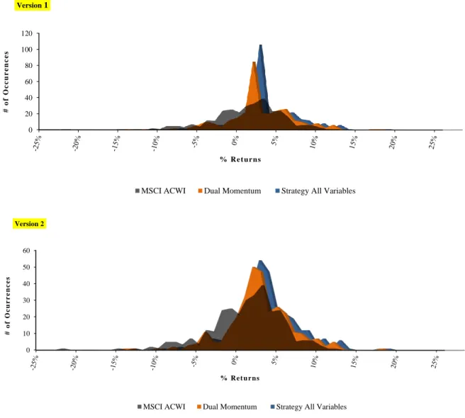
Figure 9 presents the distribution of monthly returns. Dual momentum and the strategy all variables have fewer occurrences of returns below zero, with a large portion of the returns being concentrated between 0% and 5%. Also, they display higher occurrences of large gains, and most importantly, they avoid far left tail of big negative losses. Another perspective is offered by Figures 10 and 11, which show the drawdowns and returns associated to the strategy all variables compared to those of the MSCI ACWI index and the dual momentum. During bear market environments, the ability to preserve wealth that is displayed both by the strategy and dual momentum is remarkable. For different time-horizons up to one year, the maximum drawdown inflicted to the investor is reduced by 28% in an one-month rolling basis, and by more than 60% when considering a six-month period. In the second version, the strategy all variables cuts the rolling 12-month maximum drawdown by 72% to -18%, and offers a positive return of 4.4% during down years for the MSCI ACWI which compares to +2.7% of dual momentum and a loss of 18% in the case of the benchmark index.
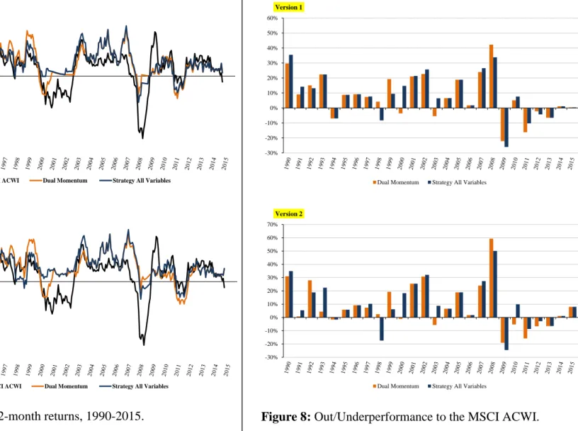
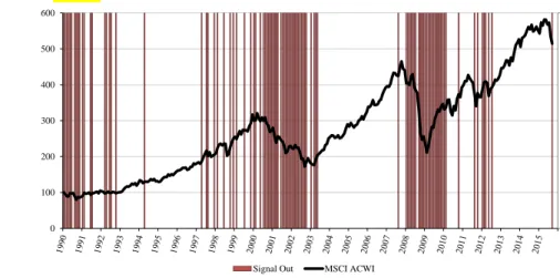
Figure 12 illustrates the effectiveness of the aggregate signal triggered by the indicators included in the strategy all variables. The most impressive improvement occurs in bear market environments and during large financial crashes. The strategy anticipates the 2000, 2001, 2002 and the 2008 severe losses, achieving an outperformance relative to the benchmark of 18.3%, 25.4%, 32.1% and 50.1% respectively, under version 2 setup. This reveals the flexibility of adjustment of the strategy, which switches from an 81% exposure to equities during bull markets to a 38% exposure as global equities trend down.
Still considering version 2 approach, we proceed to investigate to what extent does the historical outperformance of the strategy all variables over dual momentum depends on the
inclusion of the four additional indicators. Starting with the correlations between indicators, Table 5 shows that absolute momentum, which is the central component in the dual momentum model, displays a positive but low correlation (30% to 40%) with volatility and trailing EPS indicators. Moreover, momentum is negatively related to the signals of the variables linked to the interest rates, specifically -32.9% with the 3-month T-Bill yield and -6.4% with the yield spread. Between 1990 and 2015, the aggregate signal which combines all the five indicators recorded a 61.3% correlation with the absolute momentum component, 60.6% with EPS, 50.5% with volatility, 3.5% with the yield spread and -1.7% with the 3-month T-Bill.
Table 6 clarifies the degree of assertiveness of the individual indicators and of the aggregate signal. Interestingly, we find that three indicators (volatility, EPS and 3-month T-Bill) are more effective than absolute momentum in preventing the investor from being long in equities when the market is down, and thus helping to preserve wealth. Actually, absolute momentum gives more buy/hold signals then exit signals when the subsequent returns in the global stock market are negative. The ability of absolute momentum in timing the market is felt more when equity returns are positive, as it suggests staying long in approximately 74% of those months. Overall, we see that the aggregate signal ranks first in terms of effectiveness, because in 61% of the months it makes the right call about whether the investor should be invested or not in equities. The yield spread (58%), absolute momentum (57%), EPS (56%), volatility (52%) and the variable linked to the 3-month T-Bill (45%) follow.
When translating these results into the actual stock market performance, we can see the aggregate signal compares favorably to the absolute momentum rule. This suggests that the strategy all variables which relies on the aggregate signal, beats dual momentum which incorporates only the absolute momentum rule, in terms of their ability to time the market. Table 7 breaks down the returns of the MSCI ACWI index from January 1990 until September 2015
into four different scenarios, depending on the degree of exposure to equities that is determined by the absolute momentum rule versus the position implied by the aggregate signal. In the 19 months (6%) the aggregate signal supports a long position in equities in contrast to absolute momentum, the annualized average return of the MSCI ACWI is +24.95%. Conversely, when the aggregate signal agrees in exiting equities, but absolute momentum backs an investment in equities, the annualized average return of the MSCI ACWI is -8.55%, which is worse than the average loss of 6.40% when both the aggregate signal and momentum agree to sidestep equities.
Given that the aggregate signal determines how the strategy all variables performs and the absolute momentum rule defines the investment decisions under the dual momentum approach, we can stablish a relationship between the power of the signals and the performance of the strategies. Based on the evidence presented we can definitely argue the outperformance of the strategy all variables over dual momentum is attributed to the combination of momentum, volatility and the indicators connected to the business cycle.
The contribution of each individual indicator to the aggregate signal is shown in Table 8. Even though absolute momentum incorporates the aggregate signal in more than 80% of the months, most of its contribution occurs when the strategy is long on equities. In contrast, both volatility and earnings are more proactive than momentum in keeping the strategy away from equities.
Furthermore, Table 9 shows how the strategy all variables compares to the dual momentum strategy in terms of the exposure to equities during the 20th largest monthly drawdowns for the MSCI ACWI index from 1990 throughout 2015. Considering Version 2, the strategy all variables manages to preserve capital by staying aside from equities in 16, or 80%, of those months while dual momentum do not incur on 14, or 70%, of the largest monthly losses. However this improvement in terms of downside exposure (which is more pronounced in the strategy that relies on other indicators besides momentum to invest in equities), entails a trade-off. When examining
the 20th highest monthly returns between 1990 and 2015, we see that if an investor has followed the dual momentum approach or the strategy all variables it would have only captured 8 (40%) and 7 (35%) of those gains, respectively. This drawback is revealed in Table 10. However, if we carefully observe the five largest returns in their right historical context, we can argue that the inability of the strategies to seize those large gains is associated with their longer-term investment horizon and their emphasis on capital preservation.
The nature of this timing model is linked to a preference over a more conservative investment profile (with lower downside risk), which is attained by moving to a lower-volatility asset class when equities are in an apparent down market environment and/or the economy is heading into a recession. Essentially, both strategies avoid short term volatility in the stock market, such as lengthy bear markets with only sporadic rebounds. For instance, the largest monthly return of the MSCI ACWI index occurs in April 2009, on the back of all the events related to the 2008 financial crisis. During the previous months global stock market returns were especially volatile: in January -8.90%, February -10.24%, March +7.97%. Similarly, the second and the third largest monthly return (October 2011 and May 1990) are consistent with the idea of strong market rebounds, given they took place after at least four consecutive negative months. If we compute the cumulative return of the MSCI ACWI index over those five months (June 2011 to October 2011 and January 1990 to May 1990) the performance of global equities was still very negative (10.37% and -6.69%).
VI. Conclusions
The strategy developed in this paper shows that to some extent market timing can be effectively performed when just a few indicators are taken into consideration.
Furthermore, the results show that simple and easy to implement rules may help the investor to dynamically adjust his portfolio’s exposure across different geographies and between equities and bonds. This paper also confirms that the momentum profitability has persisted throughout time which supports the idea that it is the “premier anomaly” from the modern financial markets.
Our strategy comfortably outperforms the most popular proxy of global equities over a long-term investment horizon. It achieves higher average returns, reduces volatility and lowers drawdowns, and provides a large upgrade on a risk-to-reward basis relative to a buy-and-hold strategy. Moreover, it improves the dual momentum approach in nearly all performance-related indicators, and therefore beats the benchmark by an even larger margin.
In addition, the strategy offers four main advantages. Firstly, it can be implemented in real-time without constraints related to data availability because it depends only on ex-ante information. Secondly, the costs to implement and manage the strategy should be minimal due to the low turnover of the model (on average, three to four trades a year) and because it can be performed using ETFs, which in principle are as liquid as stocks6 and have lower operating expenses and a better tax treatment over actively managed funds. Thirdly, because the indicators are simple and were not subject to any optimization procedures, the strategy minimizes data mining and overfitting bias. Finally, its quantitative nature protects the investor from common behavioral biases and mental traps, as the binary nature of the indicators (invest/do not invest in
6
According to BlackRock Inc., ETFs attracted a record amount of $347 billion globally in 2015, with investors using them to replace derivatives (including futures and swaps). The ETF industry is now worth close to $3 trillion.
equities) forestalls discretionary decisions. Actually, the strategy helps an investor to take advantage of emotional and behavioral biases displayed by others.
From an investor standpoint, we can recognize this strategy may appear less attractive for two reasons. Firstly, in contrast to the traditional sense of diversification, the strategy is diversified across market cycles more than across asset classes. In fact, each month we are invested in only one asset according to the signals of the model. Secondly, it may be difficult for an investor to ignore emotions and drastically change from an all stock to an all bond portfolio, based on a systematic set of rules. However, the main caveat of this and all investment strategies is that any performance metric is based on historical data, which tells only what has happened in the past and thus it does not predict nor guarantee future returns. Indeed, investors should keep in mind that nothing will work all the time and in every circumstance. For instance, Table 4 shows that the outperformance of the strategy over the benchmark seen in the most recent years falls short to that of previous years.
Nevertheless, past performance suggests that an investor can be relatively confident in terms of downside exposure and capital protection when executing this strategy. Its effectiveness in maximizing long-term wealth is remarkable taking into consideration that was a very dynamic and volatile period: economic expansions and steep recessions, speculative bubbles, market crashes, financial scandals, bail-outs, the sovereign debt crisis, exponential growth of new asset classes, decisive monetary policy actions, ascendancy of China as world financial power, commodities prices boom and slump.
References
Antonacci, Gary. 2014. Dual momentum investing: an innovative strategy for higher returns with lower risk. McGraw-Hill Education.
Asness, Cliff, John Liew, and Ross Stevens. 1997. “Parallels between the cross-sectional predictability of stock and country returns.” Journal of Portfolio Management, 23 (3), pp. 79-87.
Asness, Cliff, Tobias Moskowtiz, and Lasse H. Pedersen. 2013. “Value and momentum everywhere.” Journal of Finance, 68 (3), pp. 929-985.
Ball, Ray, and Philip Brown. 1968. “An empirical evaluation of accounting income numbers.” Journal of Accounting Research, 6 (2), pp. 159-178.
Barberis, Nicholas, Andrei Shleifer, and Robert Vishny. 1998. “A model of investor sentiment.” Journal of Financial Economics, 49 (3), pp. 307-343.
Barroso, Pedro, and Pedro Santa-Clara. 2012. “Momentum has its moments.” Working Paper. Bhojraj, Sanjeev, and Bhaskaran Swaminathan. 2006. “Macromomentum: Returns predictability
in international equity indices.” Journal of Business, 79 (1), pp. 429-451.
Bordo, Michael, and David Wheelock. 2006. “When do stock market booms occur? The macroeconomic and policy environments of 20th century booms.” Federal Reserve Bank of St. Louis Working Paper Series.
Breen, William, Lawrence Glosten, and Ravi Jagannathan. 1989. “Economic significance of predictable variations in stock index returns.” Journal of Finance, 44 (5), pp. 1177-1189. Chabot, Benjamin, Eric Ghysels, and Ravi Jagannathan. 2009. “Momentum cycles and limits to
arbitrage evidence from Victorian England and post-depression US stock markets.” NBER Working Paper, 15591.
Chordia, Tarun, and Lakshmanan Shivakumar. 2002. “Momentum, business cycle, and time-varying expected returns.” Journal of Finance, 57 (2), pp. 985-1019.
Conover, Mitchell, Gerald Jensen, and Robert Johnson. 1999. “Monetary environments and international stock returns.” Journal of Banking and Finance, 23, pp. 1357-1381.
Conrad, Jennifer, and Gautam Kaul. 1998. “An anatomy of trading strategies.” Review of Financial Studies, 11, pp. 489-519.
Daniel, Kent, David Hirshleifer, and Avanidhar Subrahmanyam. 1998. “Investor psychology and security market under-and overreactions.” Journal of Finance, 53 (6), pp. 1839-1885.
Daniel, Kent, and Tobias Moskowitz. 2012. “Momentum crashes”. Working Paper.
De Long, J. Bradford, Andrei Shleifer, Lawrence H. Summers, and Robert J. Waldmann. 1990. “Noise trader risk in financial markets.” Journal of Political Economy, 98 (4), pp. 703-738. Fama, Eugene, and G. William Schwert. 1977. “Asset returns and inflation.” Journal of
Financial Economics, 5, pp. 115-146.
Fama, Eugene, and Kenneth French. 1989. “Business conditions and expected returns on stocks and bonds.” Journal of Financial Economics, 25 (1), pp. 23-49.
Fama, Eugene, and Kenneth French. 1993. “Common risk factors in the returns on stocks and bonds.” Journal of Financial Economics, 33 (1), pp. 3-56.
Fama, Eugene, and Kenneth French. 2008. “Dissecting Anomalies.” Journal of Finance, 63 (4), pp. 1653-1678.
Faber, Mebane T. 2013. “A quantitative approach to tactical asset allocation.” Working Paper. Grundy, Bruce D., and J. Spencer Martin. 2001. “Understanding the nature of the risks and the
source of the rewards to momentum investing” Review of Financial Studies, 14 (1), pp. 29-78. He, Wen, and Maggie Hu. 2014. “Aggregate earnings and market returns: International
Hong, Harrison, and Jeremy C. Stein. 1999. “A unified theory of underreaction, momentum trading and overreaction in asset markets.” Journal of Finance, 54 (6), pp. 2143-2184
Hurst, Brian, Yao Hua Ooi, and Lasse H. Pedersen. 2012. “A century of evidence on trend-following investing.” AQR Capital Management, LLC.
Jegadeesh, Narasimhan, and Sheridan Titman. 1993. “Returns to buying winners and selling losers: Implications for stock market efficiency.” Journal of Finance, 48 (1), pp. 65-91.
Jegadeesh, Narasimhan, and Sheridan Titman. 2001. “Profitability of momentum strategies: An evaluation of alternative explanations.” Journal of Finance, 56 (2), pp. 699-720.
Konchitchki, Yaniv, and Panos Patatoukas. 2014. “Accounting Earnings and Gross Domestic Product.” Journal of Accounting and Economics, 57, pp. 76-88.
Kothari, S.P., Jonathan Lewellen, and Jerold Warner. 2006. “Stock returns, aggregate earnings surprises, and behavioral finance.” Journal of Financial Economics, 79, pp. 537-568.
Li, Li, and Zuliu F. Hu. 1998. “Responses of the stock market to macroeconomic announcements across economic states.” IMF Working Paper, 98/79.
Liu, Laura X., and Lu Zhang. 2008. “Momentum profits, factor pricing, and macroeconomic risk.” Review of Financial Studies, 21 (6), pp. 2417-2448.
McQueen, Grant, and V. Vance Roley. 1993. “Stock prices, news, and business conditions.” Review of Financial Studies, 6 (3), pp. 683-707.
Moskowitz, Tobias, Yao Hua Ooi, and Lasse H. Pedersen. 2012. “Time series momentum.” Journal of Financial Economics, 104 (2), pp. 228-250.
Rapach, David, Jack Strauss, and Guofu Zhou. 2013. “International stock market return predictability: What is the role of the US?” Journal of Finance, 68 (4), pp. 1633-1662.
Appendix I
Figure 1: Organogram of Millennium BCP’s WMU.
Figure 2: Comparison between US and the Rest of the World in terms stock market capitalization, from 1995 to 2014.
Table 1: Distribution of weights by geography in the MSCI All-Country World Index (as at 30th September 2015) versus those of the absolute momentum strategy. The weights in the latter are derived from those in the former, by calculating the relative proportions.
Wealth Management Unit Strategy Structured Products Funds Selection Risk Control 0% 50% 100%
MSCI USA MSCI ACWI excl. USA
USA Japan Europe Excl UK EM Total %
MSCI ACWI 55% 8% 16% 10% 89%
Absolute Momentum 62% 9% 18% 11% 100%
Wealth Management Advisory Unit
Figure 3: The logic behind the Strategy All Variables.
II
I
Each Month Look at These 5 conditions
Absolute Momentum : MSCI USA > 1-month T-Bill
: MSCI USA > Barclays Agg. Bond Index
Yield Curve Not Inverted
Volatility MSCI USA < 10% 3-month T-Bill Low and Declining
EPS High and Rising
: Buy/Hold 1-month T-Bill
: Buy/Hold Barclays Agg. Bond Index Buy/Hold the Best Equity Index
(based on Relative Momentum)
MSCI USA MSCI Europe (excl. UK)
MSCI Japan MSCI EM If at Least 3 of These 5 Conditions Are True
Table 2: Performance overview, January 1990 to September 2015.
Table 3: Performance overview, January 1990 to September 2015.
Absolute Momentum 9,7% 9,9% 0,69 1,21 1,11 $1.076 -8,5% 23,9% 73% 0,8 93% Relative Momentum 10,2% 19,9% 0,37 0,58 1,17 $819 -62,3% 35,5% 63% 2,7 100% Dual Momentum 14,2% 15,1% 0,74 1,34 1,90 $2.822 -23,3% 44,6% 74% 2,2 79% MSCI ACWI 6,2% 15,6% 0,21 0,33 - $356 -54,2% 30,3% 61% - 100% Apr-90 Strategy All Variables 14,8% 14,3% 0,83 1,54 2,04 $3.450 -20,3% 44,6% 78% 3,5 70% Strategy Volatility + EPS 12,0% 12,7% 0,71 1,36 1,34 $1.770 -17,4% 44,6% 80% 3,5 Strategy Yields + EPS 13,6% 13,6% 0,78 1,48 1,74 $2.584 -17,4% 42,2% 81% 4,5 $100 becomes Maximum Drawdown, Year Maximum Return, Year % Profit, Months Trades per year Information Ratio Sortino Ratio Sharpe Ratio Annual Std Dev Annual Return 61% 59% % of Time in Equities Version 1 Absolute Momentum 9,7% 9,9% 0,69 1,21 1,11 $1.076 -12,4% 25,8% 70% 1,1 91% Relative Momentum 10,2% 19,9% 0,37 0,58 1,17 $819 -62,3% 35,5% 63% 2,7 100% Dual Momentum 14,8% 14,0% 0,85 1,56 2,00 $3.454 -23,0% 43,1% 68% 2,7 72% MSCI ACWI 6,2% 15,6% 0,21 0,33 - $356 -54,2% 30,3% 61% - 100% 0,97 1,91 1,82 $3.146 1,86 Strategy All Variables Strategy Volatility + EPS 14,2% 12,3% 0,92 Strategy Yields + EPS Information Ratio Annual Return Annual Std Dev Sharpe Ratio Sortino Ratio 1,75 $2.693 0,83 1,58 13,7% 13,0% -15,8% 44,6% 69% 3,7 -15,8% 38,5% 67% 4,7 -15,8% 46,0% 69% 3,3 68% % of Time in Equities 57% 56% Maximum Drawdown, Year Maximum Return, Year % Profit, Months Trades per year 2,35 $5.056 $100 becomes 16,3% 13,7% Version 2
Absolute Momentum
Relative Momentum Dual
Momentum Yields + EPSStrategy Strategy Volatility + EPS Strategy All Variables 0,0 0,2 0,4 0,6 0,8 1,0 1,2 0 1 2 3 4 5 S h a rp e R a ti o # Tra d e s p e r y e a r Ve r s i on 2
Figure 4: Strategies’ Sharpe ratio versus the number of trades required, on average, per year, 1990-2015. Absolute Momentum Relative Momentum Dual Momentum Strategy Yields + EPS Strategy Volatility + EPS Strategy All Variables 0,0 0,2 0,4 0,6 0,8 1,0 1,2 0 1 2 3 4 5 S h a rp e R a ti o # Tra d e s p e r y e a r Ve r s i on 1
Figure 5: $100 Investment, January 1990 to September 2015. Figure 6: Differences in cumulative growth, 1990-2015.
$50 $500 $5.000
Version 1 Dual Momentum Strategy All Variables MSCI ACWI
$50 $500 $5.000
Version 2 Dual Momentum Strategy All Variables MSCI ACWI
-1,0 5,0 11,0 17,0 23,0
Version 1 Dual Momentum Strategy All Variables
-1,0 5,0 11,0 17,0 23,0
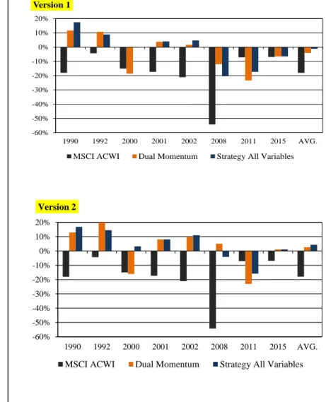
Figure 7: Rolling 12-month returns, 1990-2015. Figure 8: Out/Underperformance to the MSCI ACWI. -80% -60% -40% -20% 0% 20% 40% 60% Version 1
MSCI ACWI Dual Momentum Strategy All Variables
-80% -60% -40% -20% 0% 20% 40% 60% Version 2
MSCI ACWI Dual Momentum Strategy All Variables
-30% -20% -10% 0% 10% 20% 30% 40% 50% 60% Version 1
Dual Momentum Strategy All Variables
-30% -20% -10% 0% 10% 20% 30% 40% 50% 60% 70% Version 2
0 10 20 30 40 50 60 # o f O c u r r e n c e s % R e t u r n s Version 2
MSCI ACWI Dual Momentum Strategy All Variables
Figure 9: Distribution of monthly returns, from January 1990 to September 2015. 0 20 40 60 80 100 120 # o f O c c u r e n c e s % R e t u r n s Version1
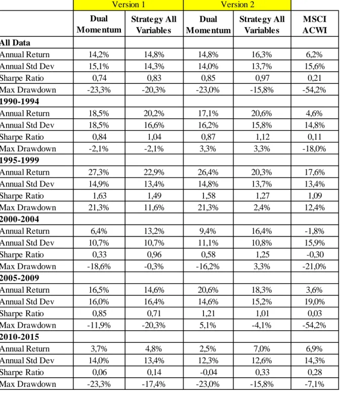
Table 4: Performance break down by sub-periods, from January 1990 to September 2015. Dual Momentum Strategy All Variables Dual Momentum Strategy All Variables MSCI ACWI All Data Annual Return 14,2% 14,8% 14,8% 16,3% 6,2% Annual Std Dev 15,1% 14,3% 14,0% 13,7% 15,6% Sharpe Ratio 0,74 0,83 0,85 0,97 0,21 Max Drawdown -23,3% -20,3% -23,0% -15,8% -54,2% 1990-1994 Annual Return 18,5% 20,2% 17,1% 20,6% 4,6% Annual Std Dev 18,5% 16,6% 16,2% 15,8% 14,8% Sharpe Ratio 0,84 1,04 0,87 1,12 0,11 Max Drawdown -2,1% -2,1% 3,3% 3,3% -18,0% 1995-1999 Annual Return 27,3% 22,9% 26,4% 20,3% 17,6% Annual Std Dev 14,9% 13,4% 14,8% 13,7% 13,4% Sharpe Ratio 1,63 1,49 1,58 1,27 1,09 Max Drawdown 21,3% 11,6% 21,3% 2,4% 12,4% 2000-2004 Annual Return 6,4% 13,2% 9,4% 16,4% -1,8% Annual Std Dev 10,7% 10,7% 11,1% 10,8% 15,9% Sharpe Ratio 0,33 0,96 0,58 1,25 -0,30 Max Drawdown -18,6% -0,3% -16,2% 3,3% -21,0% 2005-2009 Annual Return 16,5% 14,6% 20,6% 18,3% 3,6% Annual Std Dev 16,0% 16,4% 14,6% 15,2% 19,0% Sharpe Ratio 0,85 0,71 1,21 1,01 0,03 Max Drawdown -11,9% -20,3% 5,1% -4,1% -54,2% 2010-2015 Annual Return 3,7% 4,8% 2,5% 7,0% 6,9% Annual Std Dev 14,0% 13,4% 12,3% 12,6% 14,3% Sharpe Ratio 0,06 0,14 -0,04 0,33 0,28 Max Drawdown -23,3% -17,4% -23,0% -15,8% -7,1% Version 1 Version 2
Figure 10: Maximum drawdowns, 1990-2015. Figure 11: Drawdowns during MSCI ACWI down years. -70% -60% -50% -40% -30% -20% -10% 0%
1-month 3-month 6-month 12-month
Version 1
MSCI ACWI Dual Momentum Strategy All Variables
-70% -60% -50% -40% -30% -20% -10% 0%
1-month 3-month 6-month 12-month
Version 2
MSCI ACWI Dual Momentum Strategy All Variables
-60% -50% -40% -30% -20% -10% 0% 10% 20% 1990 1992 2000 2001 2002 2008 2011 2015 AVG. Version 1
MSCI ACWI Dual Momentum Strategy All Variables
-60% -50% -40% -30% -20% -10% 0% 10% 20% 1990 1992 2000 2001 2002 2008 2011 2015 AVG. Version 2
0 100 200 300 400 500 600 Version 2
Signal Out MSCI ACWI
Figure 12: MSCI ACWI performance and months when the Strategy All Variables is out of equities based on the aggregate signal.
Table 5: Correlations between indicators.
0 100 200 300 400 500 600 Version 1
Signal Out MSCI ACWI
Version 2 Abs Mom Volatility Trailing EPS 3-month T-Bill Yield Spread Aggregate
Abs Mom 1 Volatility 37,7% 1 Trailing EPS 33,0% 28,3% 1 3-month T-Bill -32,9% -25,0% -26,3% 1 Yield Spread -6,4% -14,4% -12,5% 20,2% 1 Aggregate 61,3% 50,5% 60,6% -1,7% 3,5% 1
Table 6: Effectiveness of the individual indicators vs Effectiveness of the aggregate signal.
Table 7: Market timing ability.
Table 8: Percent of the months the individual indicators coincide with the aggregate signal.
Version 2 Abs Mom Volatility Trailing EPS 3-month T-Bill Yield Spread Aggregate
56% 45%
Sell Signal and Positive Returns Buy Signal and Negative Returns
Sell Signal and Negative Returns
Correct Signal Buy Signal and
Positive Returns 45% 26% 35% 23% 57% 52% 56% 45% 27% 13% 18% 17% 58% 61% 12% 27% 21% 22% 2% 17% 38% 23% 16% 35% 26% 38% 4% 16%
Version 2 # Months % of Months
Absolute Momentum = Sell and
Aggregate Signal = Buy Absolute Momentum = Buy and
Aggregate Signal = Buy Absolute Momentum = Sell and
Aggregate Signal = Sell Absolute Momentum = Buy and
Aggregate Signal = Sell
32 10%
19 6%
11,29% 190 61%
-6,40% 68 22%
Average Return MSCI ACWI (annualized)
24,95%
-8,55%
Version 2
Contribution to Aggregate Signal Buy Sell Buy/Sell
61% 22% 83% 50% 29% 79% 38% 31% 69% Yield Spread 64% 2% 66% 27% 19% 46% Absolute Momentum Volatility Trailing EPS 3-month T-Bill