365
Selection of grids for weed mapping1 Recebido para publicação em 7.9.2014 e aprovado em 1.12.2014.
2 UNIOESTE, Cascavel-PR, Brasil, <ricardo_camicia@hotmail.com>; 3 UNICENTRO, Departamento de Agronomia, Guarapuava-PR, Brasil; 4 UTFPR, Medianeira-PR, Brasil.
S
ELECTION OFG
RIDS FORW
EEDM
APPING1Seleção de Grades para Mapeamento de Plantas Daninhas
CAMICIA, R.F.M.2, MAGGI, M.F.2, SOUZA, E.G.2, JADOSKI, S.O.3, CAMICIA, R.G.M.4,and MENECHINI, W.2
ABSTRACT - Thisstudy aimed to assessthe degree of similaritypresentedbythematic maps
generated by different sampling grids of weed plants in a commercial agricultural area of 7.95 hectares. Monocotyledons and dicotyledons were counted on the 2012/2013 and
2013/2014 harvests, before soybean planting, in the fallow period after wheat harvest, in both years. A regular gridof10 x 10 m was produced to sample the invasive plants,used as reference,and the counting was donein 1 m² of eachsample point, totaling795 samples in each year, compared toregulargridsof 30 and 50m, generated from thedata exclusion of thestandard grid. Twenty-two compositesoil sampleswere takenat a depth of0-20 cm to correlate soil properties with weeds occurrence. For the generation of the thematic maps,
the Inverse Distance Weighting (IDW)for interpolation was used; when comparing the maps generated from each grid with the reference map, the kappa coefficient was used to assess theloss of qualityof the mapsasthe number of sample points was reduced. It was observed that the map quality losswas lowerin 2013compared to2012 whenthe sampling densityof the points was reduced. The 30x30 m grids have satisfactorily described the infestation data of the dicotyledonsandthe 50 x 50mgridshave adequatelydescribed the monocotyledon weeds infestation,comparedto the standard10 x 10 m grids.
Keywords: precision agriculture, sample grids, weeds.
RESUMO - Este trabalho objetivou avaliar o grau de semelhança apresentado pelos mapas temáticos gerados por diferentes grades amostrais de plantas espontâneas em uma área agrícola comercial com 7,95 hectares. Realizou-se a contagem de monocotiledôneas e dicotiledôneas nas safras 2012/ 2013 e 2013/2014, antes do plantio da soja, período de pousio após a colheita de trigo de ambos os anos. Foi gerada uma grade regular de 10x10 m para amostragem das invasoras, utilizada como referência, sendo feita a contagem em 1m² de cada ponto amostral, totalizando 795amostras em cada ano, comparadas com grades regulares de 30 e 50m, geradas a partir da exclusão de dados da grade padrão. Foram retiradas 22amostras compostas de solo a profundidade de 0-20 cm para correlacionar atributos do solo com plantas espontâneas. Para a geração dos mapas temáticos, utilizou-se o interpolador inverso do quadrado da distância; na comparação dos mapas gerados a partir de cada grade com o mapa de referência, utilizou-se o índice kappa para avaliar a perda de qualidade dos mapas ao se diminuir o número de pontos amostrais. Observou-se que as perdas de qualidade dos mapas foram menores em 2013, em relação a 2012, quando reduzida a densidade amostral de pontos. As grades de 30x 30m descreveram de forma satisfatória os dados de infestação das dicotiledôneas, e as grades de 50x50 m descreveram adequadamente as infestações de plantas espontâneas de monocotiledôneas, quando comparadas com a grade padrão de 10x10m.
INTRODUCTION
Precision agriculture (PA) has as a key element the spatial variability of production and related factors, while traditional systems treat the soil of farms evenly, based on the average conditions of extensive cultivation areas to plan the corrective actions of the factors limiting production (Molin, 2001).
Ortiz (2010) reports that the spatial distribution analysis of the variables allows the distinction of regions with lower and higher variability and the generation of maps of a differentiated application of agricultural inputs, taking into account the amount of nutrients necessary for optimal development of the crop and the amount available in the areas of the field, providing maximum productivity, improved standardization of production and increased efficacy of the resources used.
The interference of the also called weeds is one of the main factors that lead to a reduced productivity in crops. It is known that the competition between crops and weeds causes losses averaging 15% of the world production of grains, besides the fact that they can be hosts for pests and diseases (Embrapa, 2009).
Shiratsuch et al. (2005) have described the spatial continuity structure of the population of weeds and of the seed bank, establishing a correlation between them, which has made it possible to make inferences about future infestations. Nordmeyer et al. (1997) suggest that this contagious distribution is mainly due to aspects of the weeds biology, such as soil moisture, topography, soil types, crop productivity and others. Therefore, as most weeds infest agricultural areas in “coppices”, the idea of mapping their distribution in the field has occurred, for the purpose of treatments at variable rates, such as spatial variability studies of weeds.
Geostatistical studies of the distribution of weeds allow their mapping (Cardina et al., 1996; Schaffrabthi et al., 2007) and even the adoption of localized management practices (Milani et al., 2006; Souza et al., 2008), which can reduce the amount of herbicides applied (Balastreire & Baio, 2001).
As for using PA in controlling weeds, Moraes et al. (2008) have reported that the future prospects in Brazil are promising. These authors have observed that, as studies are done incorporating the various fields of knowledge involved, there are cheaper equipment and technology compatible with the imported ones, thus ensuring lower costs.
The ability to describe and map the spatial distribution of weeds is the first step in determining the best method for the localized application of herbicides (Balastreire & Baio, 2001; Garibay et al., 2001). The decision to control weeds is based on the assessment of the real need for control (Voll et al., 2003).
In this context, this study aimed to verify the spatial distribution of spontaneous monocotyledon and dicotyledon plants in different sampling grids in commercial farming areas, comparing the loss of quality of the maps of weeds with the reduction of sample points and the existence of a spatial correlation between the physical and chemical attributes of the soil and the weeds.
MATERIALS AND METHODS
The data used in this study were collected on a farm. This area was chosen at random and was not influenced in management techniques applied by the producer as to the items to be assessed: occurrence of dicotyledon and monocotyledon weeds. Selection took into account only features such as access, the area size and the cultivation system, in order to facilitate soil and weeds samples, as they were done in 2012 and 2013. The assessments were conducted in the Brazilian post-harvest winter crop and pre-drying summer crop periods (October-November).
The sample area is 7.95 ha (hectares) wide, located in the Brazilian municipality of Realeza-PR, with central geographical coordinates of longitude of 53o 33' 00" W and latitude of 25o 42' 17" S and an average elevation of 455 m.
months and there is not a well defined dry season. The average temperature is above 22 oC in the summer and around 18 oC in the winter. The average rainfall is 2,300 mm year-1 (data from the weather station in the Salto Caxias plant – Nova Prata do Iguaçu, PR).
The sampling area, referred to as area “A”, is 7.95 ha (hectares) wide. It is located in the Brazilian municipality of Royalty, PR, with central geographical coordinates of longitude of 53o 33' 00" W and latitude of 25o 42' 17" S and an average elevation of 455 m. Wheat (Triticum aestivum) was sown in the study area, with a physiological cycle of about 120 days, on May 25, 2012. For weed management of the winter crop, was used metsulfuron-methyl post-emergence (4 g ha-1). The harvest was done on September 28, 2012.
From October 12 to 14, 2012, weed sampling was carried out (15 days after harvest). Subsequently, on October 18, 2012, the producer did the desiccation with 2 L ha-1 of glyphosate + 1 L ha-1 of 2.4 D before sowing of summer crops, soybean (Glycine max) with a physiological cycle of approximately 130 days, which was sown on October 28, 2012 (10 days after desiccation). After the soybean crop, the area was desiccated on May 15, 2013 with 2 L ha-1 of glyphosate + 1.5 L ha-1 of 2,4 D. On July 20, 2013, white oat (Avena sativa) was sown, with a physiological cycle of about 120 days for the purpose of green manure. The oatmeal was desiccated with 2 L ha-1 of glyphosate in an early grain filling phase. Samples of weeds were performed on October 14, 2013.
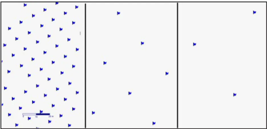
The area was measured and georeferenced with a GPS Garmim 76CSx, with an approximate precision of 2 m. Later, a regular grid of 10 x 10 m was established in the TrackMaker PRO software, which was used as a basis for the generation of other grids: an intermediate grid of 30 x 30 m and the maximum grid of 50 x 50 m for the samplings of the invasive plants. The same data were used for both grids, only the exclusion of the intermediate data was done to generate the grids of 30 m and 50 m (Figure 1). Thus, maps with lower sampling densities were obtained. The study area has 795 sample points for the grid of 10 x 10 m. For the grid of 30 x 30 m, 76 sampling points; the grid of 50 x 50 m contains 22 sample points.
Four samplings with a 0.5 x 0.5 m metal frame were randomly performed in a radius of 5 m around each sample point in an infestation level count in 1 m² for georeferenced sample, totaling 795 sampling points of invasive plants count in each year.
To interpret the results and prepare the maps, the data were tabulated and ranked in infestation levels in three classes: low, average and high, for monocotyledons and dicotyledons, according to the number of weeds found in a sample (1 m²) (Table 1). For the class ranges was used information from Vidal et al. (2010) and Patel et al. (2010), which suggest that efforts should be concentrated on estimating the impact of weeds when present in densities between 1 and 20 plants m-2, because in this range are most of the economic damage levels caused by various species of weeds.
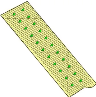
Soil samples were collected at the crossing points of a regular grid of 50 x 50 m, georeferenced and collected with an auger to a depth of 20 cm (Molin, 2001; Souza, 2008). Twenty-two 22 composite soil samples were taken with a Dutch auger to a depth of 20 cm (Figure 2).
Spatial correlation tests were performed using the program SDUM at 5% to verify the correlation between monocotyledon and dicotyledon infestations of each year with the chemical attributes (copper, zinc, iron, manganese, boron, carbon, aluminum, calcium magnesium, phosphorus, potassium and pH), also of each year; and physical attributes (sand, silt and clay) of the soil to verify the existence of an interaction between them (Bazzi et al., 2013).
To generate the thematic maps the Inverse Distance Weighting (IDW) for interpolation was used in the second power, using the interpolation window for 10 neighbors (Bazzi et al., 2013) in the SURFER 8.0 software. As better sampling quality is expected the higher the number of points, the grid of 10 m was selected for having the largest sample density as a reference to calculate the loss of quality of the maps by the kappa coefficient.
According to Carvalho et al. (2001), the kappa coefficient ranges from 0 to 1 (0 indicates that the results happen completely at random and 1 indicates complete compliance), being defined by Equation 1 (Spezia et al., 2012):
K
=
{
n
∑
i−¿1
r
x
ii−
∑
i=1
r
(
x
i+. .
x
+i)
}
{
n
2−
∑
i=1
r
(
x
i+..
x
+i)
}
(eq. 1)where: r = number of rows in a cross-classification table; xii = number of combinations diagonally; xi = total observations in row i; x+i = total observations in column j; and n = total number of observations.
Landis & Koch (1977) have suggested the following interpretation to the values of the kappa coefficient (Table 2).
The kappa coefficient is one of the most used and effective parameters to quantify the precision of land-use surveys (Spezia et al., 2012). The justification is that the goal was to estimate clearances of thematic maps using other interpolators, such as the Inverse Distance Weighting (IDW).
Table 1 - Rating of the infestation levels for monocotyledons and dicotyledons
Source: Adapted from Vidal et al. (2010) and Patel et al. (2010).
Figure 2 - Soil sampling points defined in a grid of 50 x 50 m in the study area.
Table 2 - Level of compliance of the kappa coefficient (k)
RESULTS AND DISCUSSION
The average of broad-leaves for the area in 2012 was of 5.35 plants m-2; in 2013 it was of 1.98 plant m-2. There was an average reduction in broad-leaved plants, which was probably due to the use of more efficient herbicides to control broadleaf plants such as 2.4 D and metsulfuron-methyl, as suggested by Agostinetto et al. (2008). For the narrow leaves attribute, the average values were 5.92 and 1.62 plants m-2 in the years 2012 and 2013, respectively.
In 2012, a large amount of weeds emerging from wheat was observed in the three areas studied, originating from the culture previously installed there. Thus, the reduction in the average of narrow-leaved plants is due to the use of efficient herbicides to control narrow-leaved plants like glyphosate, and also to the fact that in 2012 there was frost in the region during the reproductive phase of the wheat crop. Lower density grains were not able to be harvested and were lost during the track phase of harvesters, remaining in the studied sites, providing highest averages for that year.
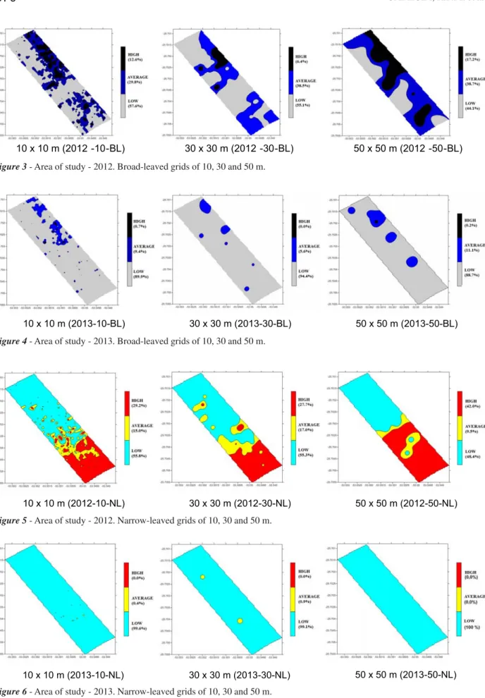
The maps representing the three levels of infestation of the years 2012 and 2013 of the area studied for broad-leaved plants (BL) and narrow-leaved (NL) for grids 10, 30 and 50 meters are shown in Figures 3 to 6.
In 2013, an increase in the areas of low infestation was observed compared to 2012 for broad-leaves (32.3%), comparing maps 2012-10-BL and 2013-2012-10-BL (Figures 3 and 4), and for narrow-leaves (43.8%), comparing maps 2012-10-NL and 2013-10-NL (Figures 5 and 6 – 50 x 50 m).
Figure 3 is the representation of map 2012-10-BL, in which is possible to see a low infestation (less than 5 plants m-2) in 57,6%, average infestation (5 to 10 plants m-2) in 29.8% and high infestation (over 10 plants m-2) in 12,6%, in relation to the total area, representing, respectively, 4.58, 2.37 and 1.0 hectares, in area measurement. This map is visually similar to 2012-30-BL (Figure 3 – 30 x 30 m), with low, average and high infestation of 55.1% (4.38 ha), 38.5% (3.06 ha) and 6.4% (0.51 ha), respectively. As for map 2012-50-BL (Figure 4), it is possible to see low
infestation levels of 44.1% (3.51 ha); average 38.7% (3.07 ha); and high 17.2% (1.37 ha). Visually maps 2012-10-BL and 2012-30-BL are similar, but a kappa coefficient of 0.32 can be seen (Table 3), ranked as partial compliance. The comparison of maps 2012-10-BL and 2012-50-BL does not present a good visual compliance, which was confirmed by the kappa coefficient value of 0.30, ranked as partial compliance, in which the overall precision was of 55.7%, meaning that only 55.7% of the ranking of map 2012-10-BL was repeated in map 2012-50-BL, which is due to the reduction of the sampling density.
In 2013 the best comparison for the BL maps was seen for the grids of 10 and 30 m in the broad-leaved plants (maps 2013-10-BL and 2013-30-BL), which have obtained an overall precision of 90.0%, with a kappa coefficient of 0.52 (moderate compliance). The difference between the kappa coefficient and the overall precision results from the elimination of the compliance due to the randomness for the calculation of the kappa coefficient. Similar results were found by Vilela et al. (2005) in mapping the spatial distribution of weeds in soybean culture by means of remote sensing, which had a kappa coefficient of 48.04% and overall precision of 70.90%.
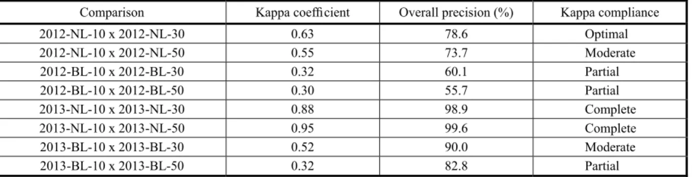
In Table 3 are shown the values of the kappa coefficient and overall precision for the classification, according to Landis & Koch (1977), for comparisons of the maps generated with different grids (10, 30 and 50 m) for the study area.
Figure 3 - Area of study - 2012. Broad-leaved grids of 10, 30 and 50 m.
Figure 4 - Area of study - 2013. Broad-leaved grids of 10, 30 and 50 m.
Figure 5 - Area of study - 2012. Narrow-leaved grids of 10, 30 and 50 m.
were similar to the ones by Normeyer et al. (1997), who have mapped weeds by sampling methods in 13 ha, using a grid of 30 x 30 m, which was considered adequate for the analysis of the data.
In the study area in years 2012 and 2013 a reduction in the amount of details in the maps generated with different grids was observed, proportional to the increase in the size of the sampling grid, due to the lower density of samples and also to the fact that weeds are distributed in an aggregated basis, allowing their mapping. These results were similar to those found by Chiba et al. (2010) when mapping the spatial variability of weeds using precision farming tools using 10 x 10 m cells, divided into three classes of infestation, who concluded that there was a defined spatial dependency structure for plants separated according to the type of leaf and for their total number. The maps obtained in this study show the aggregated pattern of spatial distribution of weeds. It was possible to define management zones with differences of infestation that were five to ten times the total number of weeds, confirming the hypothesis that the geostatistical analysis can be used as an auxiliary tool in the management.
In 2013, there was an increase in the areas of low infestation compared to 2012 for the two factors studied (narrow-leaved and broad-leaved), which occurs due to the more efficient use of herbicides in controlling weeds such as glyphosate for narrow leaves and 2.4 D and metsulfuron-methyl for broad-leaves (Agostinetto et al., 2008; Patel et al., 2010;
Maciel, 2011). Hence, these factors together have possibly reduced the average levels of infestation throughout the two years of study in the area.
The results, according to Coelho et al. (2009) and Spezia (2012) confirm the study of the work, in which the IDW was satisfactory in the interpolation for weeds, but this can be difficult in areas where infestation levels are low, leading to an underestimation, since it has a set of data with low amplitude. Thus, by reducing the sample density, the interpolator could generate maps underestimating values and neglecting areas or foci of average and high infestation, leading to failures in field control, which would entail losses in the management of invasive plants.
The results of this study indicate that the use of larger grids for description of broad-and narrow-leaves is possible. According to Balastreire & Baio (2001), the localized application, depending on the mapping of the spatial distribution of weeds, can result in savings of up to 32% related to the acquisition of herbicides.
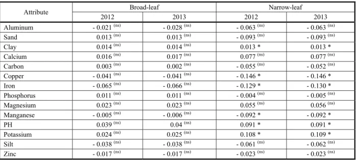
Table 4 presents the spatial correlation values for narrow- and broad-leaves with attributes aluminum, sand, clay, calcium, carbon, copper, iron, phosphorus, magnesium, manganese, pH, potassium, silt and zinc.
According to the data in years 2012 and 2013, the broadleaf parameter showed no correlation with the soil attributes for the study area. Regarding narrow-leaves, in both years there was a significant correlation
Table 3 - Kappa coefficient and overall precision of the comparisons of the different grids
for six of the soil attributes (clay, copper, iron, manganese, pH and potassium). The repetitions of the significance of the correlations for the two years was due to the fact that the soil and invasive plants samples were taken at the same sampling points set up in the two years and also because there was no agricultural lime applications in the study area, which confirms the existence of a spatial dependence of the weeds.
Monocotyledon roots develop mainly in the surface layer with a high degree of root branching and formation of secondary roots, which allows the roots to exploit a greater volume of soil, making them more sensitive and explaining the correlation with more attributes of the soil than the dicotyledons (Richart et al., 2005).
Considering the conditions in which the experiments were performed, the mapping was adequate and feasible to be done due to the aggregated distribution structure of the weeds. The grids that best described the information from the reduction of sampling points were of 50 x 50 m for the monocotyledons and of 30 x 30 m for the dicotyledons. Only the monocotyledons have shown correlations with the soil attributes. Due to possible variations of the data found in studies of weeds, it is
suggested that, for each sampling area studied, be done a sampling in an area that is representative of the land to verify the behavior of the infestation data regarding the distribution of these plants and to determine the technical and economically most feasible grid to apply in every situation, so that no invasive plant is neglected in the process of preparing the maps.
ACKNOWLEDGMENT
To Coordenação de Aperfeiçoamento de Pessoal de Nível Superior (Coordination of Improvement of Higher Education) (CAPES) for granting a scholarship to the first author and for the important financial support for the development of this work.
LITERATURE CITED
AGOSTINETTO, D. et al. Período crítico de competição de plantas daninhas com a cultura do trigo. Planta Daninha, v. 26, n. 2, p. 271-278, 2008.
BALASTREIRE, L. A.; BAIO, F. H. R. Avaliação de uma metodologia prática para o mapeamento de plantas daninhas. R. Bras. Eng. Agríc. Amb., v. 5, n. 2, p. 349-352, 2001.
BAZZI, C. L. et al. Management zones definition using soil chemical and physical attributes in a soybean area. Eng. Agríc., v. 33, n. 3, p. 1-14, 2013.
Table 4 - Spatial correlation between broad-leaf and narrow-leaf and soil attributes during the years under study, in different areas of analysis
CARDINA, J.; SPARROW, D. H.; McCOY, E. L. Spatial relationships between seedbank and seedling populations of common lambsquarters (Chenopodium album) and annual
grasses. Weed Sci., v. 44, n. 3, p. 298-308, 1996.
CARVALHO, J. R. P.; VIEIRA, S. R.; MORAN, R. C. C. P. Análise de correspondência – uma ferramenta útil na comparação de mapas de produtividade. Campinas: Empresa Brasileira de Pesquisa e Agropecuária, 2001. 4 p. (Comunicado Técnico, v. 14)
CHIBA, M. K.; GUEDES FILHO, O.; VIEIRA, S. R. Variabilidade espacial e temporal de plantas daninhas em Latossolo Vermelho argiloso sob semeadura direta. Acta Sci. Agron., v. 32, n. 4, p. 735-742, 2010.
COELHO, E. C. et al. Influência da densidade amostral e do tipo de interpolador na elaboração de mapas temático. Acta Sci. Agron.,v. 31, n. 1, p. 165-174, 2009.
EMPRESA BRASILEIRA DE PESQUISA
AGROPECUÁRIA – EMBRAPA. Plantas daninhas causam danos evitáveis. Agosto 2009. Disponível em: <http://www.embrapa.br/imprensa/noticias/2009/agosto/3a-semana/plantas daninhascausam-danos-evitaveis>. Acesso em: 10 mar. 2013.
GARIBAY, S. V. et al. Extent and implications of weed spatial variability in arable crop fields. Plant Produc. Sci., v. 4, n. 4, p. 259-269, 2001.
INSTITUTO BRASILEIRO DE GEOGRAFIA E ESTATÍSTICA – IBGE. Base Pública de Dados. Caderno estatístico do município de Realeza. 2012. p. 1-30. Disponível em: <http://www.educadores.diaadia.pr.gov.br/ arquivos/File/cadernos_municipios/realeza2012.pdf>. Acesso em: 6 abr. 2013.
LANDIS, J. R.; KOCH, G. G. The measurement of observer agreement for categorical data. Biometrics, v. 33, n. 1, p. 159-174, 1977.
MACIEL, C. D. G. et al. Eficiência e qualidade da aplicação de glyphosate + carfentrazone no controle de Commelina diffusa em função da ponta de pulverização e ação do
adjuvante triunfo Flex®. In: SIMPÓSIO INTERNACIONAL SOBRE GLYPHOSATE, 3., Botucatu, 2011. Anais... Botucatu: FEPAF, 2011. p. 388-391.
MILANI, L. et al. Unidades de manejo a partir de dados de produtividade. Acta Sci. Agron., v. 28, n. 4, p. 591-598, 2006.
MOLIN, J. P. Agricultura de precisão – o gerenciamento da variabilidade. Piracicaba: 2001. 83 p.
MORAES, P. V. D.; AGOSTINETTO, D.; GALON, L.; PIESANTI, R. Agricultura de precisão no controle de plantas daninhas. Revista da FZVA, v. 15, n. 1, p. 1-14, 2008.
NORDMEYER, H.; HÄUSLER, A.; NIEMANN, P. Patchy weed control as an approach in precision farming. In: EUROPEN CONFERENCE ON PRECISION
AGRICULTURE 97, 1., 1997, Warwick. Proceedings… London: BIOS Scientific Publications, 1997. p. 307-314.
ORTIZ, B. V. et al. Geostatistical modeling of the spatial variability and risk areas of Southern root-knot nematodes in relation in soil properties. Geoderma, Author manuscript, 2010. p. 19.
PATEL, F. et al. Nível de dano econômico de buva (Conyza bonariensis) na cultura da soja. In: CONGRESSO
BRASILEIRO DA CIÊNCIA DAS PLANTAS DANINHAS, 27., Ribeirão Preto, 2010. Resumos... Ribeirão Preto: FUNEP, 2010. p. 1670-1673.
RICHART, A. et al. Compactação do solo: causas e efeitos.
Semina: Ci. Agr., v. 26, n. 3, p. 321-344, 2005.
SCHAFFRATHI, V. R. et al. Variabilidade espacial de plantas daninhas em dois sistemas de manejo de solos. R.Bras. Eng. Agríc. Amb., v. 11, n. 1, p. 53-60, 2007.
SHIRATSUCHI, L. S.; FONTES, J. R. A.; RESENDE, A. V. Correlação da distribuição espacial do banco de sementes de plantas daninhas com a fertilidade dos solos.
Planta Daninha, v. 23, n. 3, p. 429-436, 2005.
SOUZA, G. S. et al. Variabilidade espacial de atributos químicos em um Argissolo sob pastagem. Acta Sci. Agron., v. 30, n. 4, p. 589-596, 2008.
SPEZIA, G. R. et al. Model to estimate the sampling density for establishment of yield mapping. R. Bras. Eng. Agríc. Amb., v. 16, n. 4, p. 449-457, 2012.
VIDAL, R. A. et al. Nível crítico de dano de infestantes em culturas anuais. Porto Alegre: Evangraf, 2010. 133 p.
VILELA, M. F.; FONTES, J. R. A.; SHIRATSUCHI, L. S. Mapeamento da distribuição espacial de plantas daninhas na cultura de soja por meio de sensoriamento remoto. Planaltina: Embrapa Cerrados, 2005. 26 p.(Boletim de Pesquisa e Desenvolvimento).
VOLL, E.; ADEGAS, F. S GAZZIERO, D. L. P.;