http://dx.doi.org/10.12988/ams.2015.54339
Ageing Living Individuals from Longitudinal Data
of Dental and Skeletal Maturation: A First Attempt
Marina A. P. Andrade
Departamento de Matem´atica, University Institute of Lisbon (ISCTE - IUL) BRU-IUL, Portugal
Hugo F. V. Cardoso
Department of Archaeology, Simon Fraser University, Burnaby, British Columbia, Canada
Copyright c 2015 Marina A. P. Andrade and Hugo F. V. Cardoso. This article is distributed under the Creative Commons Attribution License, which permits unrestricted use, distribution, and reproduction in any medium, provided the original work is properly cited.
Abstract
The current need in the forensic community to provide accurate age estimates for living individuals stimulates the testing and development of new approaches. The purposed guidelines suggest that a dental and skeletal age estimate should be provided, but the expert usually has to rely on two estimates obtained from different methods that cannot be combined, and the final judgment is based on a more subjective assessment of which age is more reliable or how the two estimates can be combined.
The purpose of this study is to discuss the use of panel data models to develop age estimation methods that rely on a combination of dental and skeletal maturation in a longitudinal sample of French-Canadian children between the ages of 7 and 15 years old, for legal purposes. It is intended to find out if some conjectures about possible models are true and which variables are more important in the models that perform well.
It is presented and discussed the use of random-effects models which was proven to be the correct choice for the problem in study. In the search for the best combination of variables that allows to obtain a
model to estimate the age young males around 16 years two were se-lected. For the model with better results it is evaluated how much percentage of variability explained is lost when the number of variables is reduced.
In what concerns the determinant variables in the model to estimate the age of juveniles, for the bones variables it was demonstrated that ulna is fundamental in the model as opposed to radius, which proved to be much less important. Equivalently, the third molar is a primacy variable to consider in any model for the age estimation. For the score index variables the results are either much inferior to the chosen models or, surprisingly, without any interest.
Keywords: Age estimation, panel data, fixed effects, random effects
1
Introduction
For over a decade, European forensic experts have been faced with the need to estimate the age of living individuals, due to the increase numbers of illegal cross-border crossings that involve immigrants with no identification docu-ments or proof of birth date. Very early on in 2000 this resulted in the cre-ation of the Study Group on Forensic Diagnostics of the German Associcre-ation of Forensic Medicine. The members of this group comprise forensic physicians, dentists, radiologists and anthropologists who have developed guidelines to support expert opinion and harmonization of the different approaches, to as-sure the quality of the forensic age reports.
In criminal proceedings involving illegal immigrants of doubtful age the issue involved is that of criminal liability and the age threshold of criminal responsibility differs from country to country. Regardless of the age threshold the guidelines developed by the Study Group on Forensic Diagnostics have been adopted across Europe and recommend that an age estimated based on dental maturation and another age estimate based on skeletal maturation must be provided. The expert report should present the most probable age of the individual under examination, or the probability that the stated age is the correct age or even that the individuals age is either above or below the penal age limit. However, the dental and skeletal ages cannot currently be combined because they are derived from different sources and one cannot be determined to be more accurate than the other. Consequently, the age estimation is often reported based on all the partial diagnoses and a critical discussion of the individual case. Generally each case is different from any other but the experts need to issue an evaluation of the most likely age in each case.
The central question around the most suitable examination methods for forensic application in living individuals, relies on the reference studies that can
be used to develop forensic age estimation methods, particularly those that can provide empirical evidence for combining dental and skeletal age assessment, which are currently lacking or are inexistent.
In this study we wish to examine how to proceed with statistics and the presentation of results in a legal context, particularly on how to proceed and present the age estimation for an individual using a panel data models ap-proach. From an original data set of several individuals, male and female, observed through several years in different variables – stature, skeletal and dental, and some score indexes computed for the skeletal and the dental vari-ables – a data set, which will be presented in detail in section 2, was defined to use in this work.
Here it is important to discuss the use of panel data models to determine on how to proceed in a matter of age estimation in living male individuals. The most common applications using panel data are in the domain of economic, econometric, finance, marketing and several others social sciences. In this work the observations respect human measurements in a set of male juveniles. The interest is to analyze how longitudinal observations on the stature, dental and skeletal indicators may contribute to the age estimation of an individual.
The main objective is to decide which model can be used to determine if a boy is under or over a certain age, here will be considered 16 years, consider-ing the observed values for the most informative bone and dental indicators. Together with the main purpose some conjectures will be evaluated, about the possible models and which variables are more important and interesting, to decide if an individual is 16 year old or more. Also, for the case of some lack of information; i.e., the use of a restricted number of variables, what would be an interesting alternative model and the results that may be obtained.
Still there is no scientific approach acceptable that makes use of a combina-tion of methods for age estimacombina-tion using stature, dental and skeletal indicators. There are studies on which data collected on either dental and skeletal indi-cators, see [1], [2] and [3], but there is not yet a study where all the required features for a reference population have been combined. In [4] the authors essayed an initial approach to do it but only in preliminary studies. Here it is intended to proceed further on this subject.
As mentioned in section 2 is presented the data set to be used and pointed out the decisions and conditionalities of the data set. Section 3 describes the methodology adopted to approach the problem. The results and models are exhibited in section 4. Finally, section 5 a discussion on the results obtained and some references.
2
The Data
The sample utilized comprises 25 French-Canadian boys between the age of 7 and 15 years old, derived from the Electronic Encycolpedia on Maxillo-Facial, Dental and Skeletal Development, developed at the University of Montreal by Dr. Arto Demirjian, see [5]. Each boy was assessed annually and several developmental measures were recorded. For the purpose of this study, only chronological age, height, scores of dental maturation (Demirjian-s method, for which one of eight stages of development was assigned), and scores of hand-wrist skeletal maturation (TW2 method, for which one of nine stages of development was assigned), were retained and analyzed. Since the sample is longitudinal, a total of 220 annual observations were used.
In original data set some of the individuals or the variables have non ob-served values. Thus it was necessary to make some decisions in order to reduce and solve the problem of missing observations. Also the original data set was not a sample randomly drawn in the population of young juveniles. Though the individuals biological development and consequently the variables states observations may be admitted to be random in what concerns the individuals’ insertion in the data set.
From a biological and practical point of view there are some variables com-bination that are more reasonable and interesting to explore, as models and models comparison. To overcome the problem of non observed values it was decided to replace the values of some variables by the mean value of that variable for each age of the individuals, except for the variable third molar de-velopment (M3). Being so, its non observation may be biologically explained. Thus for the third molar, it was decided not replace for the mean age of the variable when it was not observed, in a first moment and also to replace when the individual exhibits a previous observation in a previous age.
In the 25 individuals there are 6 for which M3 has not any observation, in other 5 cases there were observation in the previous age and the replace-ment was made with the aim of comparing the results with those obtained for the recorded observations of M3. For the variable M2 (second molar) there were 5 replacements and again the computations were made with and without replacements, for comparison.
For the stature variables – Height and Weight – all the individuals have complete observations, as well as the skeletal variables – Radius and Ulna. In the remaining variables, the dental and skeletal score indexes and ages – variables TW2 Age, Rus Age, TW2 Score, Rus Score, Demirjian Age and Demirjian Score – it was made 1 replacement in Tw2 Score and 12 replace-ments in Demirjian Age and Demirjian Score. For each individual there is also a variable named ID referring the individuals identification during the 9 years of observation - the panel variable.
3
Methodology: Panel Data Models
Panel (or longitudinal) data are cross-sectional and time-series data sets with multiple entities, each of which has repeated measurements at different time periods. Panel data may have group effects, time effects, or the both, which are analyzed by fixed effect and random effect models. A panel data set contains n entities or subjects, such as firms and states or individuals, each of which includes T observations measured at 1 through t time period. Therefore, the total number of observations is nT . Generally, panel data are measured at regular time intervals – year, quarter, and month. Panel data have a cross-section (entity or subject) variable and a time-series variable, thus panel data models study fixed and/or random effects of individual or time.
The central difference between fixed and random effect models is based on the role of dummy variables. In a fixed effect model a parameter estimate of a dummy variable is a part of the intercept whereas it is an error component in a random effect model. The slopes remain the same across group or time period in either fixed or random effect model. Thus, the functional form of a panel data regression model may be written as:
yit= α + Xit0β + uit i = 1, ...n, t = 1, ..., T . (1)
with uit= µi+ νit
Where i denotes the cross-section dimension, t denotes denotes the time-series dimension, α is a scalar, β is a K × 1 and Xit is the it-th observation on K
explanatory variables.
The use of panel data models is presented mainly in applications of Econo-metric data sets. The spread of this models use has been done with examples referring econometric problems involving measurements over time of compa-nies, countries and when referring individuals mots of the time measuring their wage and salaries, income from self-employment, etc. Here the variables ob-servation refer to obob-servations of human stadiums with respect to skeletal or dental development in young males. This will have significance in the choice of the models to use.
The fixed effect model examines group differences in intercepts, assuming the same slopes and constant variance, across subjects. Since a group (indi-vidual specific) effect is time invariant and considered a part of the intercept, µi is allowed to be correlated to other regressors. Fixed effect models use least
squares dummy variable (LSDV) and within effect estimation methods. Or-dinary least squares (OLS) regressions with dummies, in fact, are fixed effect models. In the fixed effect model there are too many parameters to estimate and consequently a loss of degrees of freedom in the model.
The random effect model estimates variance components for groups (or time) and error, assuming the same intercept and slopes, µi is a component of
the errors and consequently should not be correlated to any regressor; other-wise, a core OLS assumption is violated. The difference among groups stays in their variance of the error term and not in their intercepts. The random effect model is estimated by generalized least squares (GLS) when the vari-ance structure matrix, among groups, is known. When the varivari-ance structure matrix is not known the feasible generalized least squares (FGLS) method is used to its estimate. Compared to fixed effect models, random effect models are relatively difficult to estimate. A random effect model examines how group and/or time affect error variances. This model is appropriate for n individuals who were drawn randomly from a large population.
The use of fixed effects or random effects model is of no importance when T is large, because both the LSDV estimator and FGLS estimator become the same estimator. However, if T is finite and n is large to threat the effects as fixed or random is not an easy decision.
As it is stated in [6] the advantage of fixed-effects inference is that there is no need to assume that the effects are independent of xi. The
disadvan-tage is that it introduces the issue of incidental parameters. The advandisadvan-tage of random-effects inference is that the number of parameters is fixed and effi-cient estimation methods can be derived. The disadvantage is that one has to make specific assumptions about the pattern of correlation (or no correlation) between the effects and the included explanatory variables.
3.1
A Random-Effects Model Choice
A random-effects model assume that the individual’s (or entity’s) error term is not correlated with the predictors which allows for time-invariant variables to play a role as explanatory variables. In random-effects it is necessary to specify the characteristics that may or may not influence the predictor vari-ables. A problem that may arises is that some variables may not be available, consequently leading to omitted variables bias in the model. An advantage of the random-effects model use is that it allows to generalize the inferences beyond the sample used in the model.
In this paper the option has focused on using the random effects model, essentially supported by biological criteria. For the problem concerned the existing data are measurements in human units, young males. Thus, in ac-cordance with what is considered biological measurements, both in continuous scale like height, weight and scale of stages - qualitative converted to discrete values, the effects are random. It is assumed that the errors ui are not
corre-lated with the regressors.
de-cision supported more on biological considerations and justifications, it can be evaluated if the decision was according with the presumptions considered above. Thus, to decide between fixed-effects and random-effects one can use the Hausman test to decide. So, the null hypothesis is that the preferred model is random-effects versus the alternative hypothesis of fixed-effects. The test mainly intends to find out whether the unique errors are correlated with the regressors. In the null hypothesis they are not. If individual effects are correlated with any other regressor, the random-effects model violates a Gaus-Markov assumption and is no longer Best Linear Unbiased Estimate (BLUE). This is why individual effects are parts of the error term in the random-effects model. If the null hypothesis is not rejected, a random-effects model is favored over the fixed-effects models1
It was significative to check about the considerations made and conse-quently on cross-sectional and time-series variables to determine if it was the right decision. For the different models tested and compared (presented and discussed in the following section) there was a suspicion, biologically sustained, that some specific ones should present better results. The results and discus-sion are presented in the following section.
3.1.1 Testing for Random-Effects
The Breusch-Pagan Lagrange Multiplier (LM) test helps to decide between a random effects regression and a simple ordinary least squares (OLS) re-gression models. Again, the use of one other diagnostic test was taken to corroborate the expectations about the problem in study. The null hypoth-esis is that individual-specific or time-specific error variance components are zero: H0 : σ2u = 0. For this, variances across entities is zero meaning that no
significant difference across units (i.e. no panel effect). If the null hypothesis is rejected the pooled OLS is preferred; otherwise, the random-effect model is the adequate model to use. Once again the results and discussion are in the next section.
4
Models Results
A purpose in this work was also to find out if some conjectures about possible models were true. If some, or any, of the score indexes variables are important as part in models that perform well. Within the more interesting models which is the better. And for an alternative model – with a shorter number of variables – which is the loss for the percentage of variability explained.
1In a fixed-effects model, the individuals effects are parts of the intercept and the
corre-lation between the intercept and regressors does not violate any Gaus-Markov assumption – a fixed-effects model is still BLUE.
In the next section are presented the results for the best models that may be used for male age estimation, using the data set described above, between the several tried models. Based on the chosen model was then tested the random-effects model using the Breusch-Pagan Lagrange Multiplier (LM) test.
4.1
The Random-Effects Model for Age Estimation
Re-sults
Among several models that were thought appropriate, some others were also considered (not shown here). From a developmental perspective it was clear that radius and ulna bones would have a contribution in the models as well as the second and third molars. Also of interest was to determine if score index variables and if so, which ones, might give a contribution for the age estimation models.
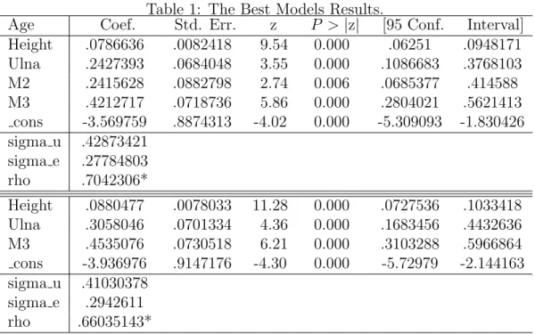
In the search for the best combination of variables that allows to obtain a model to estimate the age young males around 16 years two were selected. In the table below, table 1, are presented the models that catch the highest percentage of variability explained by the model. For all the tested models the results were obtained with the use of Stata software, as well as the tests performed to analyse and decide the models choice.
Table 1: The Best Models Results.
Age Coef. Std. Err. z P > |z| [95 Conf. Interval] Height .0786636 .0082418 9.54 0.000 .06251 .0948171 Ulna .2427393 .0684048 3.55 0.000 .1086683 .3768103 M2 .2415628 .0882798 2.74 0.006 .0685377 .414588 M3 .4212717 .0718736 5.86 0.000 .2804021 .5621413 cons -3.569759 .8874313 -4.02 0.000 -5.309093 -1.830426 sigma u .42873421 sigma e .27784803 rho .7042306* Height .0880477 .0078033 11.28 0.000 .0727536 .1033418 Ulna .3058046 .0701334 4.36 0.000 .1683456 .4432636 M3 .4535076 .0730518 6.21 0.000 .3103288 .5966864 cons -3.936976 .9147176 -4.30 0.000 -5.72979 -2.144163 sigma u .41030378 sigma e .2942611 rho .66035143*
∗ (fraction of variance due to u i)
total error variance, as it is expressed in the results output where the * indicates the fraction of variance due to u i. A large ratio means that individual specific errors account for large proportion of the composite error variance.
It is possible to notice that the model with the variables Height, Ulna, M2 and M3 exhibits about 70% of variability explained by the model. In the case the individual specific error can explain about 70 percent of the entire error variance, and can be interpreted as a goodness–of–fit of random effect model, which can be obtained as follows:
0.7042306 = 0.42873421
2
0.428734212+ 0.277848032.
The second best model may be considered a partial model of the previous one (with the variables Height, Ulna and M3). For this other model the per-centage of variability explained by the model is about 66%. As it can also be observed all the coefficients are significative, the P > |z| is zero or very close to zero for all the coefficients.
4.2
A Random-Effects Model Choice Results
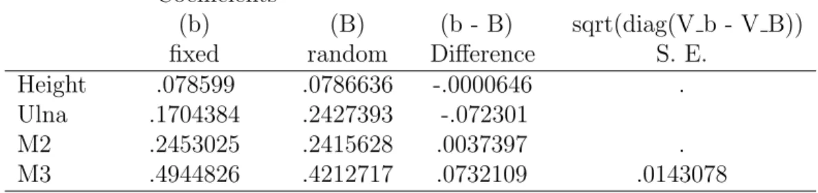
Here is presented the result of Hausman test, described in section 3.1, for model that performed better (section 4.1). To perform the Hausman test it is required that both fixed and random-effects models are fitted and stored. After run the test the result is obtained, and presented below in table 2:
Table 2: Hausman Test random-effects versus fixed-effects. — Coefficients —
(b) (B) (b - B) sqrt(diag(V b - V B))
fixed random Difference S. E.
Height .078599 .0786636 -.0000646 .
Ulna .1704384 .2427393 -.072301
M2 .2453025 .2415628 .0037397 .
M3 .4944826 .4212717 .0732109 .0143078
b = consistent under H0 and Ha;
B inconsistent under Ha, efficient under H0;
Test: H0: difference in coefficients not systematic
chi2(4) = (b - B)0[(V b - V B)ˆ(−1)](b - B) = 4.46 Prob > chi2 = 0.3471 (V b - V B is not positive definite)
As it can be seen the intuition, i.e. the origin argument in the decision of the problem, was pointing the right decision. The Prob > chi2 = 0.3471 then random-effects should be used.
4.2.1 Testing for Random-Effects Results
The estimated results of Breusch-Pagan LM test, for the model mentioned in 4.1, are presented below in table 3:
Table 3: Breusch and Pagan Lagrangian multiplier test for random effects Age[ID,t] = Xb + u[ID] + e[ID,t]
Var sd=sqrt(Var) Age 3.31293 1.820145 e .0771995 .277848 u .183813 .4287342 Test: Var(u)= 0 chibar2(01) = 87.53 Prob > chibar2 = 0.0000
With a large chi-squared of 87.53 the null hypothesis is rejected. The random-effects model is the appropriate choice (Prob > chibar2 = 0.0000). 4.2.2 The Age Estimated Results
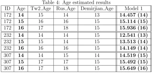
For the model with variables Height, Ulna, M2 and M3 (Model 1) are presented in table 4, for 3 individuals - 172, 232 and 307. In the table are presented also the age estimated given by the index variables Tw2 Age, Rus Age and Demirjian Age allowing to compare the age estimate results obtained by the model with the ones computed for the biological index.
For individuals with ID 172 and ID 307 the model underestimate the age, but the estimate is near the real age of the individual. Individual with ID 232 obtains real underestimated values for the age. The score indexes variables, as it can be noticed, present significative differences, though tend to overestimate the individuals’ age. So only for individual 232 the score index estimate are equal or near, but underestimate, the individual age. It is recognized that these score indexes generally overestimate the age of an individual, which raises some problems in what concerns individuals’ risk of being assigned with a higher age. On the other models that were tried, their biological interest or fundament and the results obtained is a matter to approach in the discussion section.
Table 4: Age estimated results
ID Age Tw2 Age Rus Age Demirjian Age Model 1
172 14 15 14 13 14.457 (14) 172 15 16 16 15 15.114 (15) 172 16 17 18 15 15.936 (16) 232 14 14 14 15 12.541 (13) 232 15 15 14 15 13.513 (14) 232 16 16 16 15 14.149 (14) 307 14 14 15 14 14.519 (15) 307 15 17 17 15 15.492 (15) 307 16 17 18 15 15.649 (16)
5
Discussion
As already pointed out in 4.1 the model with the variables Height, Ulna, M2 and M3 exhibits about 70% of variability explained by the model and the second best model about 66%. Clearly, variable M3 is fundamental in any model for the age estimation. As it can be noticed if variable M2 is not considered the percentage of variability explained by the model is about 66%. A loss of about 4%.
Within the bone variable, Radius proved to be the least interesting. Ap-parently, for the boys the Ulna bone is more informative in age estimation model. For the score indexes variables the results are either much inferior to the presented models or, surprisingly, without any interest. In some cases the variability explained by the model is zero, i.e. the variability present in the data is totally random error, when those variables are used in the model. This may be a consequence of the variables construction, since the index that are determined as combination of observations made on individuals, the bones in the case of Tw2 Score, Tw2 Age, Rus Score and Rus Age and and the teeth for Demirjian Score and Demirjian Age. The variability of individuals is masked and ends up working as random error.
Also important to notice, is that the results for the estimation of age pre-sented in the table 4 show that, in general, the age is underestimated for the panel data model obtained. This may be considered a conservative result that benefits the individual in the sense that it protects individuals from an age overestimation appreciation. Though, for the data available, more realistic than the estimates given by the Tw Age, Rus Age and Demirjian Age which is of major importance in legal age decisions, and works in the interest of the individuals under examination.
References
[1] A. Demish and P. Wartman, Calcification of the Mandibular Third Molar and its Relation to Skeletal and Chronological Age in Children, Child Development, 27 (1956), 459 - 473. http://dx.doi.org/10.2307/1125899 [2] K. A. Lacey, Relationship Between Bone Age and Dental
Develop-ment Lancet, 302 (1973), 736 - 737. http://dx.doi.org/10.1016/s0140-6736(73)92569-5
[3] F. F. Lamons and S. W. Gray, A Study of the Relationship Between Tooth Eruption Age, Skeletal Development Age, and Chronological Age in Sixtyone Atlanta Children, American Journal of Orthodonty, 44 (1958), 687 - 691. http://dx.doi.org/10.1016/0002-9416(58)90146-5
[4] M. Andrade and H. Cardoso, The Problem of Age Determination in Living Individuals, AIP Conference Proceedings, 1558 (2013), 1889. http://dx.doi.org/10.1063/1.4825900
[5] K. J. Reichs and A. Demirjian, A Multimedia Tool for the Assessment of Age in Immature Remains: The Electronic Encyclopedia for Maxilo-Facial, Dental and Skeletal Development. In: Reichs, K. J. Ed., Forensic Osteology Advances in the Identification of Human Remains, Charles C. Thomas Publisher, Springfield, IL, (1998), 253 - 267.
[6] C. Hsiao, Analysis of Panel Data, Cambridge University Press. Cam-bridge, 2003. http://dx.doi.org/10.1017/cbo9780511754203
[7] H. B. Baltagi, A Companion to Econometric Analysis of Panel Data, Wiley, John & Sons, England, 2001.
[8] H. M. Park, Practical Guides to Panel Data Modeling: A Step by Step Analysis Using Stata, Tutorail Working Paper, Graduate School of Inter-national Relations, InterInter-national University of Japan, (2011).
[9] A. Demirjian, H. Goldstein and J. M. Tanner, A New System of Dental Age Assessment, Human Biology, 45(2) (1973), 211 - 227.
[10] J. M. Tanner and R. H. Whitehouse, Assessment of Skeletal Maturity and Prediction of Adult Height (TW2 Method), London, U.K.: Academic Press, 1975.