Clouds and convection in the tropics and subtropics:models, observations, and parameterizations

Faculdade de Ciências

Departamento de Engenharia Geográfica, Geofísica e Energia

Clouds and Convection in the Tropics and Subtropics: Models,

Observations, and Parameterizations

Sambingo da Silva Cardoso

Doutoramento em Ciências Geofísicas e da Geoinformação

(Meteorologia)

Faculdade de Ciências

Departamento de Engenharia Geográfica, Geofísica e Energia

Clouds and Convection in the Tropics and Subtropics: Models,

Observations, and Parameterizations

Sambingo da Silva Cardoso

Tese orientada pelo Prof. Doutor Pedro Manuel Alberto de Miranda e

pelo Doutor Andrew Gettelman, especialmente elaborada para a

obtenção do grau de doutor em Ciências Geofísicas e da

Geoinformação (Meteorologia)

“Everything that is really great and inspiring is created by the individual who can labor in freedom.”

Preamble

This thesis is the result of work done by Sambingo da Silva Cardoso during his doctoral studies in Meteorology at the University of Lisbon (UL, Portugal). The investigation, performed in the framework of the GPCI (Global energy and water cycle experiment cloud system study / working group on numerical experimentation Pacific Cross-section Intercomparison) project, was carried out both in Portugal and in the United States of America (U.S.A.), respectively, at the Center of Geophysics of the University of Lisbon (CGUL), and at the National Center for Atmospheric Research (NCAR). The work was supervised by Professor Pedro Miranda (UL), and by Doctor Phil Rasch (NCAR, now at Pacific Northwest National Laboratory [PNNL, U.S.A.]), later substituted by Doctor Andrew Gettelman (NCAR). Short-term visits to the Joint Institute for Regional Earth System Science and Engineering (JIFRESSE, University of California, U.S.A.), and to the Jet Propulsion Laboratory (JPL, U.S.A.) were hosted by Doctor João Teixeira (JPL), GPCI project coordinator. GPCI was funded by the National Aeronautics and Space Administration (NASA, U.S.A.) grant X06AB74G. CGUL is funded by the Portuguese Science and Technology Foundation (FCT, Portugal). NCAR is supported by the National Science Foundation (NSF, U.S.A.). The work presented here was supported from February 2008 to February 2012 by a Doctoral Grant from FCT (SFRH/BD/37214/2007).

Scientific Articles Published in Refereed Journals

Teixeira, J., S. Cardoso, M. Bonazzola, J. Cole, A. DelGenio, C. DeMott, C. Franklin, C. Hannay, C. Jakob, Y. Jiao, J. Karlsson, H. Kitagawa, M. Köhler, A. Kuwano-Yoshida, C. LeDrian, J. Li, A. Lock, M. J. Miller, P. Marquet, J. Martins, C. R. Mechoso, E. van Meijgaard, I. Meinke, P. M. A. Miranda, D. Mironov, R. Neggers, H. L. Pan, D. A. Randall, P. J. Rasch, B. Rockel, W. B. Rossow, B. Ritter, A. P. Siebesma, P. M. M. Soares, F. J. Turk, P. A. Vaillancourt, A. Von Engeln, and M. Zhao, 2011: Tropical and Subtropical Cloud Transitions in Weather and Climate Prediction Models: The GCSS/WGNE Pacific Cross-Section Intercomparison (GPCI). J. Climate, 24, 5223–5256. Karlsson, J., G. Svensson, S. Cardoso, J. Teixeira, and S. Paradise, 2010: Subtropical cloud

regime transitions: Boundary layer depth and cloud-top height evolution. J. Appl. Meteor. Climatol., 49, 1845–1858.

Other Publications

Cardoso, S., J. Teixeira, 2009: Preliminary results from the GPCI project. Available online at: http://gcss-dime.giss.nasa.gov/gpci/modsim_gpci.html

http://gcss-dime.giss.nasa.gov/gpci/modsim_gpci_models.html

http://gcss-dime.giss.nasa.gov/gpci/GPCI-results-to-GCSS_DIME_CMAI-012008.pdf Teixeira, J., S. Cardoso, A. P. Siebesma, and the GPCI Team, 2008: Results from the First 2

Years of the GCSS Pacific Cross Section Intercomparison. GEWEX News, No. 18(4), International GEWEX Project Office, Silver Spring, MD, 1–4.

Acknowledgements

During my long doctoral journey I had the honor of meeting and interacting with a large number of people to whom I am grateful. There is not enough space here to list all of them and the ways they have helped me. From the administrative personnel at the various institutions I visited (most notably, Christina Book, at NCAR in Boulder [U.S.A.], a friend for life!), to the graduate and undergraduate students I met at some of those research centers, not forgetting the roommates and landladies I had during my stays abroad (especially, 91 years young Louise Adams, a dear friend!), or even the, always amicable, NCAR shuttle drivers, I truly believe that every single person I met during this, not always easy, journey deserves my profound appreciation.

To Professor Pedro Miranda, from the University of Lisbon (UL), I am indebted for the continued support and guidance (muito obrigado Professor!). Doctor João Teixeira, the coordinator of the GPCI project, has been crucial in helping to define the context for my doctoral work. I here acknowledge all the support and research opportunities he offered me (muito obrigado João!). Doctor Pedro Soares from the Center of Geophysics of the University of Lisbon has always been available, and provided significant guidance at important stages of my work. Doctor Pedro Viterbo, from then Portuguese Meteorological Institute, offered helpful comments on work developed during the first doctoral year. It was with great pleasure that I worked under the supervision of both Doctor Phil Rasch, and Doctor Andrew Gettelman, while at NCAR. Their friendly and informal ways gave me with much needed confidence in my research work. I additionally thank Professor José Teixeira da Silva (UL), and Professor Fernando Santos (UL), for providing me with letters of recommendation.

Many thanks go to all the GPCI collaborators, whose model simulations and observational data are the raw material for my doctoral investigation. I am especially appreciative of the interaction with Doctors Cecile Hannay and Jennifer Kay, from NCAR, Doctor Roel Neggers from the Royal Netherlands Meteorological Institute (KNMI), Doctor Johannes Karlsson from the Department of Meteorology of the Stockholm University (MISU), and Doctor Yuying Zhang from the Lawrence Livermore National Laboratory (LLNL, U.S.A.).

A few unstructured one-on-one meetings were very insightful and provided me with interesting ideas and suggestions, namely, the meetings in Boulder with Doctor George Kiladis, at the National Oceanic and Atmospheric Administration (U.S.A.), and with Doctor Gunilla Svensson (MISU), at NCAR; the meetings in Pasadena, at the Jet Propulsion Laboratory

(U.S.A.), with Doctors Edward Olsen, Eric Fetzer, and Brian Kahn; and a more recent meeting at NCAR with Doctor Peter Caldwell (LLNL / Program For Climate Model Diagnosis and Intercomparison [PCMDI], U.S.A.).

Finally, to my parents and sister, an infinite thank you for all the support and love, and, last but not least, to Doctor Sylvain Dupont: thank you for always being there (merci Vain!).

Abstract

The GPCI (GCSS / working group on numerical experimentation Pacific Cross-section Intercomparison) project offers a new approach for the intercomparison of models, by focusing the analysis on a single cross section in the NE Pacific ocean. It is targeted at the stratocumulus, shallow cumulus, and deep convection regimes, as well as the respective transitions. Three-hourly satellite observations and model simulations were prepared for GPCI for the JJA season. The seasonal mean results for variables such as total cloud cover, liquid water path, and outgoing longwave radiation show high scatter among models. Mean vertical velocity, and relative humidity, suggest good, overall, representation of the Hadley circulation. Still, differences exist between models (e.g., in the intensity of the deep convection, or humidity content in the boundary layer). The main cloud types are represented differently (e.g., too low stratocumulus clouds). The transitions between stratocumulus and shallow cumulus show two distinct behaviours (smooth versus abrupt with bimodal nature) reflecting distinct cloud parameterization approaches. None of them reproduces well the observations. Following GEPAT (Grade-based Empirical Pattern Analysis Technique), different cloud patterns were analyzed in terms of the means of associated parameters. Model relative humidity has negative biases in the boundary layer and subtropical mid troposphere. sBLT (sequential Boundary-Layer-Top determination scheme) offered a more thorough characterization of the boundary layer (top). Mean BLT height and strength show big spread among models. Models disagree in the time of the diurnal maxima of relative humidity, cloud fraction, and liquid water content. Precipitation lacks in diurnal amplitude in the deep convection area. The “Scinertia” concept was introduced, based on the analysis of diurnal cycle results for cloud cover and low tropospheric stability. GPCI proved useful for the work presented below, both in the characterization of model shortcomings, and in helping envision avenues for future investigation using models and observations.

Resumo

Apesar dos consideráveis avanços dos últimos 20 anos ao nível da parametrização de nuvens, a representação de nuvens ainda é um desfio para as comunidades de modelação do tempo e do clima. A urgência do desenvolvimento de parametrizações de nuvens para modelos de circulação geral (GCM) é reforçada pelo facto de a quantidade de nuvens gerada pelos modelos ter um impacto significativo no comportamento do sistema climático previsto pelos modelos. Em particular, os atuais modelos de clima tendem a responder de forma diferente em experiências de sensibilidade das mudanças climáticas. Deficiências nas parametrizações resultam igualmente numa representação inconsistente do ciclo hidrológico ao nível termodinâmico, o que acarreta importantes consequências para a simulação da circulação atmosférica tropical e subtropical. Estes tópicos são investigados por diferentes grupos do GCSS (Global energy and water cycle experiment Cloud System Study), cuja estratégia tem sido bem sucedida na definição e compreensão de regimes de nuvens fundamentais, e no desenvolvimento e melhoramento de parametrizações de nuvens. No entanto, o uso exclusivo de versões unidimensionais dos modelos atmosféricos, tradicionalmente feito no GCSS, não permite uma compreensão profunda do papel fundamental das nuvens no clima, o que implica que as parametrizações têm de ser testadas nas versões completas (tridimensionais) dos GCMs. Essa é uma tarefa que pode ter que envolver a análise de enormes quantidades de dados de simulações numéricas.

Neste contexto, o projeto GPCI (GCSS / working group on numerical experimentation Pacific Cross-section Intercomparison) oferece uma nova (e menos pesada) abordagem para a intercomparação de GCMs, focando a análise num número reduzido de localizações ao longo de uma secção, e permitindo uma integração de dados de modelos e de observações relativamente simples. GPCI tem estado centrado nos (sub)trópicos do sector NE do oceano Pacífico, e desenvolveu um programa especificamente dedicado à investigação de regimes de nuvens fundamentais que tipicamente ocorrem nas fronteiras orientais dos oceanos (sub)tropicais, nomeadamente, estratocúmulos, cúmulos pouco profundos, torres de convecção profunda, e as transições entre eles. O conhecimento ganho a partir de uma análise detalhada do comportamento destes sistemas de nuvens e dos ambientes dinâmicos e termodinâmicos a eles associados, recorrendo a dados de alta resolução temporal obtidos de observações e de modelos de previsão do tempo e do clima, deverá oferecer pistas para o desenvolvimento e melhoramento de novas parametrizações de nuvens, camada limite e convecção. Tendo sido

desenvolvida em estreita ligação com o projeto GPCI, a investigação apresentada nesta tese foi orientada segundo as linhas dos principais objetivos e questões científicas do projeto.

GPCI pode ser visto como um projeto de intercomparação de nível 2, em que todos os modelos participantes têm de seguir um conjunto comum de especificações e protocolos predefinidos. A condição básica imposta foi a de que os modelos deveriam correr em modo de clima, usando temperatura da superfície do mar (SST) prescrita como condição fronteira. O período de interesse corresponde a junho-julho-agosto (JJA). A região geográfica a estudar esta compreendida entre -5ºN a 45ºN e 160ºE a 240ºE, e inclui 13 localizações ao longo de uma secção. Os resultados das simulações numéricas foram pedidos numa resolução temporal de 3 horas para variáveis na forma de perfis verticais e para variáveis a um nível fixo. Mais de vinte instituições de previsão do tempo e do clima aderiram ao projeto e extensas quantidades de dados de satélite foram preparados para uso no GPCI. A análise de dados de modelos e de reanálises sugere que é possível estudar os principais aspetos da fenomenologia das nuvens, recorrendo apenas a uma secção individual alinhada com a circulação atmosférica associada à circulação da célula de Hadley na região em causa.

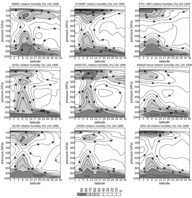
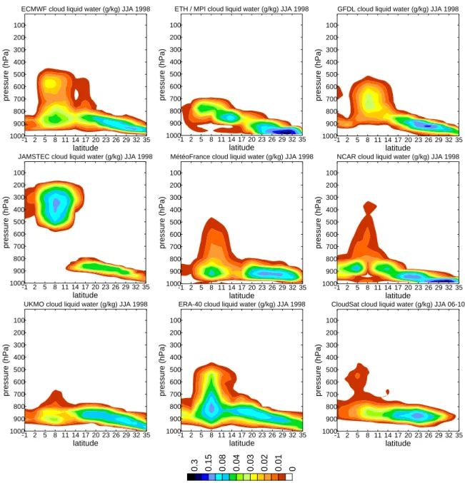
Uma análise preliminar de dados de modelos e de observações, com o objetivo de se obter uma visão geral das caraterísticas médias do ciclo hidrológico durante o verão na região GPCI, foi feita com particular enfase na distribuição vertical das nuvens, e nos processos que envolvem fatores dinâmicos e ambientais que têm um papel na manutenção dos campos de nuvens. As médias sazonais da maior parte das variáveis (e.g., cobertura nebulosa total [TCC], conteúdo de água líquida integrado na vertical [LWP], e radiação emergente de longo comprimento de onda [OLR]) são caracterizadas por um elevado grau de dispersão entre os vários modelos, que raramente mostram uma boa concordância com as observações em todos os pontos da secção. Perfis médios de velocidade vertical (w) e de humidade relativa (RH), sugerem que as características básicas da circulação atmosférica regional imposta pela célula de Hadley são, de um modo geral, bem representadas, apesar de, em detalhe, existirem diferenças substanciais entre os vários modelos (e.g., na intensidade da convecção profunda, ou no conteúdo em humidade na camada limite). Uma comparação da distribuição vertical de cobertura nebulosa (CF) nos vários modelos, mostrou bem os desafios da parametrização e simulação de nuvens em GCMs, com as simulações a mostrarem uma variedade de comportamentos ao nível da representação dos diferentes tipos de nuvens (e.g., estratocúmulos demasiado baixos) e das transições entre eles (e.g., presença de mais do que uma camada de nuvens nas áreas de transição). Estes resultados foram validados com observações da ocorrência de nuvens obtidas

com os satélites CloudSat e CALIPSO (Cloud-Aerosol Lidar and Infrared Pathfinder Satellite Observations). Um estudo ao nível dos processos físicos relevantes para as nuvens, revelou que, de um modo geral, existe uma resposta notória da circulação de larga escala a mudanças na SST prescrita nos modelos. As respostas de outras variáveis, tais como, balanço da radiação de pequeno comprimento de onda no topo da atmosfera (NSRTOA) e TCC, são ainda mais pronunciadas e variam de modelo para modelo. O facto de, na maior parte dos modelos, a resposta ao aumento da SST nem sempre ser coerente entre as diferentes variáveis, aponta para a necessidade de um melhor controlo do comportamento da simulação de importantes parâmetros relacionados com as nuvens, incluindo aqueles cruciais para a avaliação do forçamento radiativo das nuvens. Não foi encontrada (nos dados de 3-em-3 horas das simulações para JJA 1998) nenhuma relação óbvia entre as nuvens baixas (dos regimes de cúmulos pouco profundos e de estratocúmulos) a subsidência e a SST (ou mesmo a estabilidade estática da baixa troposfera [LTS]).

Foi feita uma análise de fundo da transição entre regimes convectivos, baseada no comportamento espaciotemporal das nuvens em simulações dos modelos, em reanálises e em observações de satélite. Com esse objetivo em mente, foram desenvolvidas várias técnicas para detetar transições de regime de nuvens, e ou, caracterizar a sua estrutura sazonal. Funções de distribuição de probabilidade, obtidas para TCC nas várias posições ao longo da secção GPCI, a partir de dados de 3-em-3 horas para a estação JJA 1998, mostram diferenças de modelo para modelo e apresentam importantes disparidades mesmo em posições onde os modelos mostram praticamente o mesmo valor na TCC média. Dois comportamentos distintos foram identificados ao nível da transição entre os estratocúmulos e os cúmulos dos ventos alísios: uma transição relativamente gradual da TCC; e uma variação mais abrupta, com carácter bimodal. Estes dois tipos de comportamentos são, provavelmente, um resultado da maneira como as nuvens são parametrizadas nos respetivos modelos. De qualquer maneira, nenhum destes comportamentos coincide com a forma como as transições se dão em dados correspondentes a observações da TCC do ISCCP (International Satellite Cloud Climatology Project). Estatísticas da cobertura nebulosa obtidas segundo uma metodologia desenvolvida para a deteção de fortes gradientes de TCC ao longo da secção, mostram uma diversidade de comportamentos entre os modelos, por exemplo, no valor médio do decréscimo de TCC, na sua frequência de ocorrência, ou nos histogramas da localização dessas transições em TCC (as reanálises também diferem do ISCCP). Adicionalmente, foi também efetuada uma análise espectral preliminar da série temporal correspondente a variações da localização das transições

abruptas em TCC ao longo da secção. Não tendo sido detetados picos importantes nos respetivos espectros, foi na forma da evolução temporal nas correspondentes séries, que os modelos mais se distinguiram (e.g., uma tendência, num dos modelos, para as transições ocorrerem mais para norte na secção no período final da estação JJA; ou a relativamente pequena amplitude das oscilações de localização encontradas num outro modelo). Em termos da evolução espacial da altura do topo das nuvens vista ao longo da secção, a média dos modelos está próxima dos dados de análise, apesar de, especialmente a sul das áreas de estratocúmulos, todos os resultados diferirem de observações MISR (Multiangle Imaging Spectroradiometer). Ainda no contexto da transição de regime de nuvens, foi desenvolvida uma nova abordagem de análise de padrões espaciais (GEPAT [Grade-based Empirical Pattern Analysis Technique]) com objetivo de se analisarem as condições ambientais associadas a diferentes estruturas espaciais da TCC identificadas pela nova técnica durante a estação JJA 1998. Foram assim encontrados seis diferentes padrões espaciais de cobertura nebulosa típicos da estação (cada um com diferente representatividade de ocorrência temporal). As correspondentes médias em termos de outras variáveis, tais como w aos 700 hPa, LWP, SST, LTS, e direção e intensidade do vento, foram analisadas, tendo sido encontradas diferenças, especialmente ao nível dos campos de w aos 700 hPa e LWP. Algumas ideias da aplicação futura da técnica incluem: a análise de outras estações e anos (separada ou conjuntamente); uma comparação de resultados para diferentes regiões; e o uso de dados puramente observacionais.

Foi dada especial atenção à estrutura da humidade na região GPCI, com o objetivo de uma maior compreensão do seu papel como um dos principais parâmetros no contexto do ciclo hidrológico, particularmente através da sua influência na formação e evolução das nuvens. Para esse fim, foram analisadas ao longo da secção, observações de satélite (AIRS [Atmospheric InfraRed Sounder]), simulações numéricas e análises da atmosfera, referentes a perfis de RH, obtidos para JJA (2003) na forma de médias sazonais, variância e evolução temporal. A comparação dos modelos com os dados AIRS mostrou diferenças significativas (e.g., valores bastante inferiores de RH nos níveis mais baixos da camada limite nas simulações, valores mais elevados do que as observações na tropopausa, e maior secura aos níveis médios da atmosfera nas regiões subtropicais nos modelos). No que diz respeito ao desvio padrão, ainda que, de um modo geral, os modelos apresentem maior variabilidade de RH, existem nas simulações, valores mais baixos na camada limite ao longo de toda a secção. Pensa-se que os valores mais elevados de desvio padrão apresentados pelos modelos imediatamente acima da

camada limite a norte da região dos cúmulos pouco profundos devam estar associados primariamente à relativamente fraca resolução vertical dos dados AIRS usados (mais do que serem uma consequência de deficiências nos modelos). A evolução temporal da distribuição vertical de RH parece apontar para a necessidade de se incluir na investigação das transições entre os estratocúmulos e os cúmulos dos ventos alísios, a influência, não apenas da estrutura da humidade nas camadas da troposfera logo acima da camada limite, mas também do perfil de humidade até às camadas superiores da troposfera. Mais especificamente em relação à estrutura da humidade na baixa troposfera, foi apresentada uma nova metodologia para a determinação do topo da camada limite sobre o oceano (sBLT [sequential Boundary-Layer-Top determination scheme]). Os resultados preliminares parecem promissores, especialmente pela sua abrangente aplicabilidade, e dado que a técnica permite uma maior caracterização da camada limite (e do seu topo) que outros métodos relacionados. Médias sazonais para a altura e a intensidade do topo da camada limite foram analisadas para modelos e análises ao longo da secção GPCI, e mostram dispersão considerável, exceto em termos da (praticamente comum) taxa de subida do topo da camada limite de norte para sul entre a área dos estratocúmulos e a dos cúmulos pouco profundos. As áreas de convecção profunda e dos estratocúmulos apresentam, respetivamente, o maior e o menor grau de definição (intensidade) do topo da camada limite. Segundo a classificação sBLT, foram encontradas nos modelos, e para as várias localizações na secção, diferenças na distribuição sazonal da representatividade dos vários tipos de camada limite. A esse respeito, apenas dois dos modelos se assemelham às observações AIRS. Foi ainda desenvolvida uma versão atualizada da técnica para deteção de mudanças abruptas na cobertura nebulosa ao longo da secção. A nova metodologia pareceu apresentar maior robustez no constrangimento dos resultados dos modelos para aquelas situações que efetivamente correspondem a transições espacialmente consistentes com a definição dos regimes de nuvens característicos dos estratocúmulos e dos cúmulos dos ventos alísios. Os valores da ocorrência das transições baixou drasticamente na maior parte dos modelos, e permitiu, uma melhor identificação dos impactos que diferentes filosofias de parametrização de nuvens têm no comportamento dos modelos a este nível. Por último, foram obtidos os perfis médios de RH correspondentes a cada um dos dois regimes de nuvens identificados, tendo sido verificadas importantes diferenças entre os dois regimes, para um determinado modelo, mas também entre os modelos, principalmente na forma como diferem os seus perfis de estratocúmulos e de cúmulos pouco profundos na média e alta troposfera. Foram propostas formas concretas de se estender a investigação dos potenciais impactos da estrutura da humidade da troposfera na transição entre os regimes de nuvens.

Um dos principais tópicos para o projeto GPCI é a representação, em modelos de previsão do tempo e do clima, de variações diurnas das nuvens e de parâmetros relacionados. Essas variações foram analisadas com base em dados de 3-em-3 horas obtidos dos modelos e de observações. O ciclo diurno médio na estação JJA foi descrito para diferentes localizações na secção GPCI. Foram apresentados resultados para: circulação atmosférica associada com a dinâmica de larga escala na região do Pacífico NE dominada pela célula de Hadley; perfis verticais de vários parâmetros de interesse para as nuvens; e anomalias médias do ciclo diurno em três posições da secção, representativas dos principais regimes de nuvens/convecção que caracterizam a região. A velocidade vertical aos 700 hPa apresenta, em geral, nos modelos e análises, um ciclo diurno marcado na zona de convergência inter-tropical (ITCZ). Nalguns modelos variações diurnas mais fracas foram também encontradas na região dos ventos alísios e nas regiões subtropicais. Num dos modelos o ciclo diurno de w aos 700 hPa é praticamente inexistente em qualquer das posições ao longo da secção. A intensidade e direção do vento na baixa troposfera mostrou variações diurnas características. A distribuição vertical de RH, CF, e conteúdo em água líquida das nuvens (CLW), mostrou alguma variabilidade diurna em todos os modelos analisados, especialmente abaixo dos 600 hPa na área de convecção profunda. Os modelos não concordam na altura do ciclo diurno em que simulam os valores máximos destas variáveis. Verificou-se, em geral, uma melhor concordância entre a variação diurna de CF e CLW nos estratocúmulos e nos cúmulos pouco profundos do que na ITCZ. Há, na região subtropical num dos modelos, CF simulada sem CLW associada. Em relação às anomalias médias diurnas de LTS, TCC, e precipitação (observações deste parâmetro foram obtidas de dados TRMM [Tropical Rainfall Measuring Mission]), os modelos tendem a concordar no primeiro parâmetro, mas diferem uns dos outros, e em relação às observações, nos outros dois.(e.g., na ITCZ, a TCC do ISCCP apresenta dois máximos relativos, sendo o mais pronunciado o que ocorre cerca das 16:00h locais, enquanto que nos modelos e análises, o pico de TCC mais importante dá-se tipicamente de madrugada). Nos estratocúmulos o ISCCP (TCC) tem a menor variação diurna, sendo a esse respeito, ultrapassado pelos modelos. De qualquer maneira, é nessa região que se verifica uma maior concordância entre modelos, análises e observações na altura do ciclo diurno em que se dá o máximo de TCC. No que diz respeito à taxa de precipitação, a maior parte dos resultados mostra um pico relativamente bem definido em todas as localizações ao longo da secção, mas apresentam, para os modelos, uma fraca amplitude diurna na ITCZ comparativamente aos dados TRMM. Finalmente, foi investigada a ligação, durante o ciclo diurno, entre a LTS e a cobertura nebulosa nos estratocúmulos para o caso particular de um modelo com um esquema de parametrização que

associa os dois, tendo-se argumentado sobre a existência de um certo grau de “inércia” na resposta da cobertura nebulosa subtropical em relação às variações diurnas de LTS. Do mesmo modo, e uma vez que a resposta (positiva) das nuvens à estabilidade estática do ambiente pareceu ser mais eficaz para a altura do ciclo diurno em que o valor de TCC era o mais baixo, inferiu-se qualitativamente sobre uma possível dependência dessa resposta no valor apresentado pela cobertura nebulosa. Até que ponto estará a “Scinércia” (ou “inércia dos estratocúmulos [Sc]” em relação à LTS) relacionada com a estrutura da humidade da (média) troposfera, foi uma questão deixada para investigação futura.

Dois pontos, para concluir. Primeiro, este trabalho mostra bem como os atuais modelos de previsão numérica do tempo e do clima ainda apresentam uma deficiente representação das nuvens e de processos relacionados. Segundo, a abordagem proposta pelo projeto GPCI provou ser útil na caracterização dos principais problemas dos modelos, e na definição de possíveis linhas de investigação futura, quer ao nível da modelação, quer na frente observacional.

List of Figures

Figure 2.1 - Annual mean global distribution of low stratiform clouds (stratus, stratocumulus, and fog) obtained from surface observations (from Klein and Hartmann 1993). ... 8 -Figure 2.2 - Illustration of the main cloud regimes associated with thermally direct circulations between the

tropics, and the subtropics of the eastern boundaries of the main oceanic basins (EQ for equator) (from Stevens 2005). ... 9 -Figure 2.3 - Schematic representation of the physical and dynamical processes that affect the cloud-topped

maritime boundary layer (adapted from Garratt 1992). ... 13 -Figure 3.1 - Representation of the GCSS/WGNE Pacific cross section (black diagonal line), and ISCCP low cloud

cover (%) climatology for the JuneJulyAugust season (courtesy Dr. Cecile Hannay)... 21 -Figure 3.2 - Histograms of wind direction at 1000 hPa for six points along the GPCI transect from ERA-40 for

JuneJulyAugust (JJA) 1998... 26 -Figure 3.3 - Histograms of precipitation from the NCAR and GFDL models for one GPCI point (5°N, 195°E) and

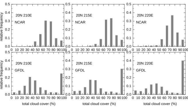
two adjacent (5° to the east and west along the same latitude) points for JuneJulyAugust 1998... 27 -Figure 3.4 - Histograms of total cloud cover from the NCAR and GFDL models for one GPCI point (20°N,

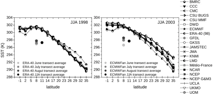
215°E) and two adjacent (5° to the east and west along the same latitude) points for June-July-August 1998. ... 28 -Figure 4.1 - Mean sea surface temperature (SST) along the GPCI transect for June-July-August (JJA) 1998 (left)

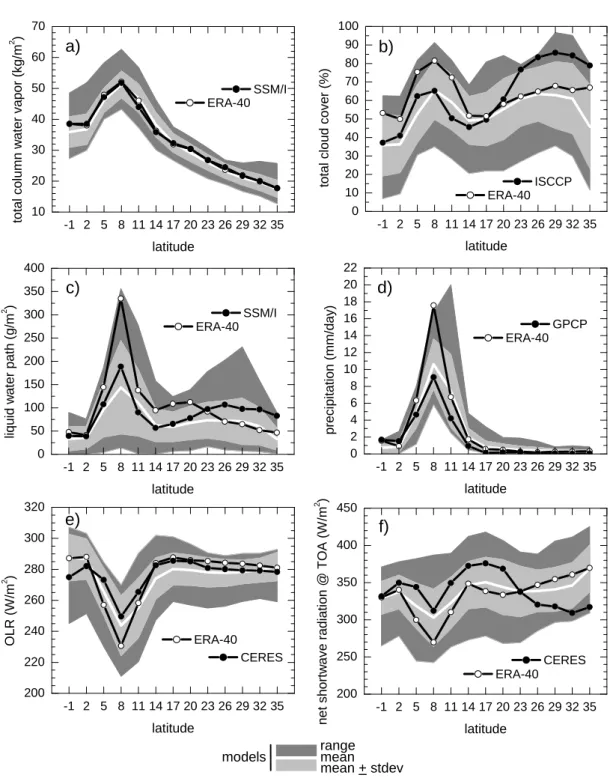
and 2003 (right) from the participating models and ECMWF analysis. ... 29 -Figure 4.2 - (a) Total column water vapor from the models along GPCI for June-July-August 1998 together with

ERA-40 and SSM/I, (b) as in (a) but for total cloud cover and ISCCP observations, (c) as in (a) but for liquid water path, (d) as in (a) but for precipitation and GPCP observations, (e) as in (a) but for outgoing longwave radiation (OLR) and CERES observations, and (f) as in (a) but for net shortwave radiation at the top of the atmosphere (TOA) and CERES observations. Results from the different models are shown as ensemble mean results, the mean plus or minus the standard deviation, and the maximum and minimum values attained by any model for a particular point (referred to as range). ... 31 -Figure 4.3 - Vertical cross sections of subsidence along the GPCI transect for June-July-August (JJA) 1998 from

models and ERA40... 35 -Figure 4.4 - Vertical cross sections of relative humidity along the GPCI transect for June-July-August (JJA) 1998

from models and ERA40. ... 36 -Figure 4.5 - Vertical cross sections of liquid water (content) along the GPCI transect for June-July-August (JJA)

1998 from models and ERA40, and for JJA 200610 for CloudSat observations. ... 38 -Figure 4.6 - Vertical cross sections of cloud occurrence along the GPCI transect for June-July-August 2006 from

CloudSat (left), CALIPSO (center), and a combination of both (right) (see text for details). ... 39 -Figure 4.7 - Vertical cross sections of cloud fraction along the GPCI transect for June-July-August (JJA) 1998

from models and ERA40. ... 40 -Figure 4.8 - Vertical velocity at 700 hPa (w700hPa), total cloud cover (TCC), liquid water path (LWP),

precipitation (P), outgoing longwave radiation (OLR), and net shortwave radiation at the top of the atmosphere (NSRTOA) along GPCI from models and ECMWF analysis (ECMWFan) composited for the months with the coolest (spatially averaged) monthly mean SST (COOL [squares]) and warmest (spatially averaged) monthly mean SST (WARM [stars]) among June, July, and August from 1998 and 2003. ... 42 -Figure 4.9 - Mean low cloud cover for jointly binned classes of vertical velocity at 700 hPa (mb) and: sea surface

temperature (left column), and low tropospheric stability (right column) along the GPCI transect (14°N to 35°N) for JuneJulyAugust (JJA) 1998 for two models and ERA40. ... 48 -Figure 5.1 - June-July-August (JJA) 1998 mean total cloud cover along GPCI from each one of the participating

models, ERA40 reanalysis, and ISCCP observations... 51 -Figure 5.2 - June-July-August (JJA) 1998 histograms of total cloud cover along the GPCI transect for some of the

-Figure 5.3 - June-July-August (JJA) 1998 ISCCP and ERA-40 cloud cover statistics obtained from a methodology based on the identification of large gradients of total cloud cover (tcc drop > 30 %) along the GPCI transect (see text for details): (left) seasonal mean values, and (right) histograms of the locations of the abrupt changes in total cloud cover (occ stands for occurrence [in percent]). ... 56 Figure 5.4 Similar to Fig. 5.3, but for some of the GPCI models... 57 -Figure 5.5 - Boundary layer height estimate based on the pressure at the top of low clouds, obtained along the

GPCI transect for June-July-August 2003, for models, ECMWF analysis [dashed line], and MISR observations [solid black line]. The solid dark-gray line represents the median of the model ensemble, the light-gray envelope represents the interquartile model range, and the dark-gray envelope represents the range of model values: (a) mean values, (b) mean values for the models individually [gray lines], and (c) temporal variability (one standard deviation). (Figure taken from Karlsson et al. 2010). ... 60 -Figure 5.6 - June-July-August (JJA) 1998 time series of the location (relative to the seasonal mean position) of

sharp gradients in total cloud cover (see text for details) for ISCCP observations, ERA-40 reanalysis, and some of the GPCI models (in the abscissa axis, minor ticks correspond to days, and labels, located at the beginning of each week during the season, indicate number of 3hourly records up to that time). ... 63 -Figure 5.7 - Frequency spectra of the June-July-August 1998 time series presented in Fig. 5.6 for ISCCP

observations, ERA40 reanalysis, and some of the GPCI models (MétéoFrance is not shown in Fig. 5.6). 65 -Figure 5.8 - ERA-40 June-July-August (JJA) 1998 seasonal mean fields of vertical velocity at 700 hPa

(W700mb), liquid water path (LWP), sea surface temperature (SST), and low tropospheric stability (LTS) along the GPCI transect, together with section-averaged wind direction (direc) and speed, composited for each one of six clustering partitions of corresponding ERA-40 GEPAT results for total cloud cover. The bottom plot shows the means for the season as a whole (this figure is analyzed in Appendix A.4). ... 67 -Figure 6.1 - Daily Atmospheric InfraRed Sounder (AIRS) relative humidity (RH) profiles along the GPCI cross

section (black diagonal line), together with 12 UTC GOES10 satellite infrared snapshots for August 7 (top row), 26 (mid row), and 30 (bottom row), 2003 (see text for details). ... 74 -Figure 6.2 - Top row: June-July-August (JJA) 2003 mean total cloud cover (red line with triangles) along the

GPCI cross section for four of the participating models (the horizontal green line marks the 70 % total cloud cover value), together with the respective percentages of occurrence of total cloud cover less than or equal to 70 % (gray columns). Bottom row: difference between constrained and unconstrained seasonal mean relative humidity (RH) (see text for details). ... 78 -Figure 6.3 - June-July-August 2003 vertical structure of relative humidity (RH) along the GPCI cross section as

seen in the mean (left plot) and standard deviation (right plot) taken from AIRS observations... 80 -Figure 6.4 - For the same four GPCI models presented in Fig. 6.2, June-July-August 2003 cross sections of

seasonal mean relative humidity (RH) (left column), RH standard deviation (std dev, in the third column from the left), and the corresponding biases versus the respective AIRS results (model - AIRS, in the second and fourth columns from the left, respectively)... 82 -Figure 6.5 - June-July-August (JJA) 2003 5-day running means of the vertical distribution of relative humidity

(RH evolution) at three different locations along the GPCI cross section (8°N, 20°N, and 32°N), for AIRS observations (top row) and two participating models (mid and bottom rows)... 84 -Figure 6.6 - Four vertical profiles of relative humidity (RH, black lines with open circles [at profile levels]), and

respective profiles of the vertical gradient of relative humidity (RH grad., gray lines with black crosses [at the mid levels of the RH profiles]). The thick solid horizontal color lines indicate particular levels in the RH grad. profiles associated with the S# indexes with the same colors (the color shown is the one for the highest S# whenever different S#s fall in the same level). The thick black solid and dash lines indicate, respectively, the 700 hPa and 650 hPa levels (see text for details)... 96 -Figure 6.7 - Mean June-July-August (JJA) 2003 boundary layer top (BLT) pressure (left plot) and strength (right

plot) along GPCI for eight participating models and ECMWF analysis (ECMWFan), determined using the sBLT methodology applied to relative humidity data (see text for details). ... 98 -Figure 6.8 - June-July-August 2003 sS# Distribution (BLT S hist.) and not7.S1 (BLT vs. 7S1) statistics along

GPCI for eight participating models and ECMWF analysis (ECMWFan), determined using the sBLT methodology applied to relative humidity data (see text for details). ... 99 -Figure 6.9 - Mean June-July-August (JJA) 2003 boundary layer top (BLT) pressure (top row left plot) and

statistics determined along GPCI using the sBLT methodology applied to AIRS relative humidity data (see text for details)... 102 -Figure 6.10 - June-July-August 2003 (jja03) statistics of total cloud cover transition (frequency of occurrence

[occ.], location histograms [histogr.], means for location and north and south averages [black line]), together with mean profiles of relative humidity (RH) averaged to the north and to the south of the transition locations found during the season between 14°N and 35°N along the GPCI cross section (see text for details). 106 -Figure 7.1 - For four of the participating models and ERA-40 reanalysis, June-July-August 1998 mean diurnal

cycle of vertical velocity at 700 hPa (w700, top row), and horizontal wind direction (to where the wind is blowing to, in degrees clockwise from North, mid row) and speed (bottom row) vertically averaged in the 1000 hPa to 850 hPa layer, all at each one of the 13 locations along GPCI, and for 8 UTC (Universal Time Coordinated) 3hourly during the day... 108 -Figure 7.2 - For four of the participating models and ERA-40 reanalysis, June-July-August 1998 mean diurnal

cycle of vertically distributed relative humidity (top row), cloud fraction (mid row), and cloud liquid water content (bottom row), for the Inter-Tropical Convergence Zone (ITCZ, 8°N) location in the GPCI transect, and for 8 UTC (Universal Time Coordinated) 3hourly during the day. ... 109 -Figure 7.3 - For four of the participating models and ERA-40 reanalysis, June-July-August 1998 mean diurnal

cycle of vertically distributed relative humidity (top row), cloud fraction (mid row), and cloud liquid water content (bottom row), for the shallow cumulus area (ShCu, 20°N) in the GPCI transect, and for 8 UTC (Universal Time Coordinated) 3hourly during the day... 110 -Figure 7.4 - For four of the participating models and ERA-40 reanalysis, June-July-August 1998 mean diurnal

cycle of vertically distributed relative humidity (top row), cloud fraction (mid row), and cloud liquid water content (bottom row), for the stratocumulus area (Sc, 32°N) in the GPCI transect, and for 8 UTC (Universal Time Coordinated) 3hourly during the day. ... 110 -Figure 7.5 - For four of the participating models, ERA-40 reanalysis, ISCCP observations, and TRMM estimates,

June-July-August 1998 mean diurnal cycle anomalies of low tropospheric stability (LTS), total cloud cover (TCC), and precipitation (P), obtained in three different areas along GPCI (Inter-Tropical Convergence Zone [ITCZ, 8°N], shallow cumulus [ShCu, 20°N], stratocumulus [Sc, 32°N]), and for 8 UTC (Universal Time Coordinated) 3hourly during the day... 112

-List of Tables

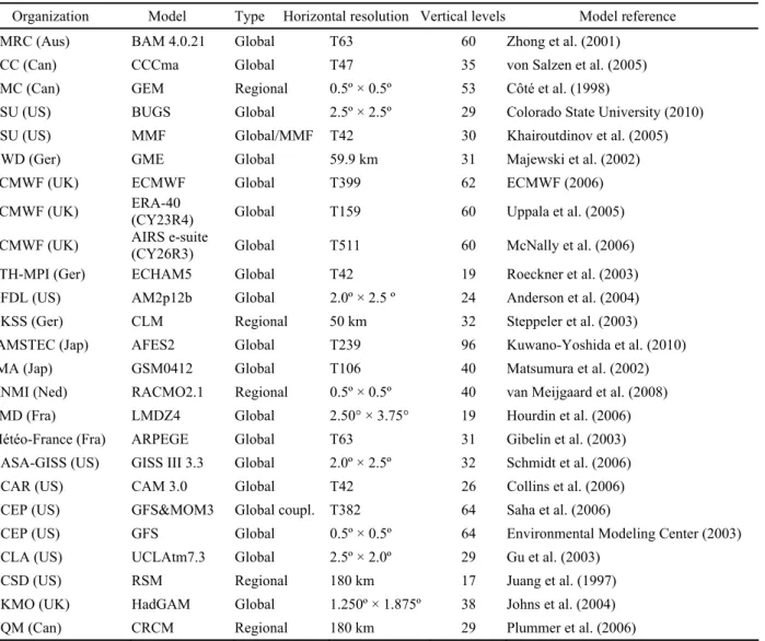
Table 3.1 - Basic information about the models that joined GPCI, with a listing of the corresponding organizations, the model name and type, the horizontal and vertical resolutions used in the simulations, and the model references. The table also lists two ECMWF analysis products (ERA-40, and AIRS e-suite [ECMWFan]).

... 23 -Table 3.2 - Basic information on observational datasets used for GPCI model evaluation. This table lists the data

center source of the observations, the dataset name, the horizontal and temporal resolutions of the data products, the parameters retrieved, and relevant product references. ... 25

-List of Acronyms and Abbreviations

1D one-Dimensional

2D two-Dimensional

3D three-Dimensional

AFES2 Atmospheric GCM for the Earth Simulator, version 2

AIRS Atmospheric InfraRed Sounder

am ante meridiem

AM2p12b Atmospheric Model, version 2p12b

AMSR-E Advanced Microwave Scanning Radiometer for the Earth observing _system

AMSU Advanced Microwave Sounding Unit

AR Absolute Roughness of the cluster-size distribution

ARM Atmospheric Radiation Measurement

ARPEGE Action de Recherche Petite Echelle Grande Echelle

ASDC Atmospheric Science Data Center

ASTEX Atlantic Stratocumulus Transition EXperiment

Aus Australia

BAM4.0.21 Bureau of meteorology unified Atmospheric Model, version 4.0.21

BL atmospheric Boundary Layer

BLH Boundary Layer Height

BLT Boundary Layer Top

BMRC Bureau of Meteorology Research Centre

BOMEX Barbados Oceanographic and Meteorological EXperiment

CALIOP Cloud-Aerosol Lidar with Orthogonal Polarization

CALIPSO Cloud-Aerosol Lidar and Infrared Pathfinder Satellite Observations CAM3.0 Community Atmosphere Model, version 3.0

Can Canada

CBL convective boundary layer

CCC Canadian Centre for Climate modeling and analysis CCCma Canadian Centre for Climate modelling and analysis CERES Clouds and the Earth’s Radiant Energy System

CF Cloud Fraction

CG Cluster Grade

CGUL Center of Geophysics of the University of Lisbon

CLM CLimate Model

CLW Cloud Liquid Water content

CMC Canadian Meteorological Centre

coupl. coupled

CP Centroid Pattern

CPR Cloud Profiling Radar

CRCM Canadian Regional Climate Model

CRF Cloud Radiative Forcing

CRM Cloud-Resolving Model

CSRM Cloud-System-Resolving Model

CSU Colorado State University

CTEI Cloud-Top Entrainment Instability

CTH Cloud-Top Height

CY23R4 model cycle 23R4

CY26R3 model cycle 26R3

DAAC Distributed Active Archive Center

DBSCAN Density-Based Spatial Clustering of Applications with Noise DD centroid-patterns’ Degree of Dissimilarity

DIME Data Integration for Model Evaluation DISC Data & Information Service Center DMSP Defense Meteorological Satellite Program

dNR degree of Normalized Roughness

DS centroid-patterns’ Degree of Similarity

DWD Deutsche WetterDienst

DYCOMS Dynamics and Chemistry of Marine Stratocumulus

E East

ECMWF European Center for Medium-Range Weather Forecasts

ECMWFan ECMWF analysis

EIS Estimated Inversion Strength

EOS Earth Observing System

EQ equator

ERA-40 ECMWF 40 Year Re-analysis

ERBE Earth Radiation Budget Experiment

ES9 ERBE-like Science product 9

ETH Eidgenössische Technische Hochschule

EUROCS European Cloud Systems Study

FCT Portuguese Science and Technology Foundation

FIRE First International satellite cloud climatology project Regional Experiment

fNR factor to Normalize the absolute Roughness of the cluster-size distribution

FOV Field Of View

FP Full Profile

Fra France

ftop pressure at the RH-profile level just above the top level of the first subprofile

GCM General Circulation Model

GCSS Global energy and water cycle experiment Cloud System Study

GEM Global Environment Multiscale

GEOPROF CloudSat Geometrical Profiling Product

GEPAT Grade-based Empirical Pattern Analysis Technique

Ger Germany

GES Goddard Earth Sciences

GEWEX Global Energy and Water cycle EXperiment GFDL Geophysical Fluid Dynamics Laboratory

GFS Global Forecast System

GISS Goddard Institute for Space Studies

GISSIII3.3 Goddard Institute for Space Studies global climate middle _{atmosphere model III, version 3.3}

GME Global Model Europe

GMS Geosynchronous Meteorological Satellite

GOES Geostationary Operational Environmental Satellite GPCC Global Precipitation Climatology Centre

GPCI Global energy and water cycle experiment cloud system study / working group on numerical experimentation Pacific Cross-section Intercomparison

GPCP Global Precipitation Climatology Project

GSFC Goddard Space Flight Center

GSM0412 Global Spectral Model, version 0412 HadGAM Hadley centre Global Atmosphere Model

ID Identification

IPCC Intergovernmental Panel on Climate Change

IPW Integrated Precipitable Water

IR InfraRed

ISCCP International Satellite Cloud Climatology Project ITCZ Inter-Tropical Convergence Zone

JAMSTEC Japan Agency for Marine-Earth Science and Technology

Jap Japan

JIFRESSE Joint Institute for Regional Earth System Science and Engineering

JJA June-July-August

JK10 Karlsson et al. (2010)

JMA Japan Meteorological Agency

jPDF joint Probability Density Function

JPL Jet Propulsion Laboratory

JSC Joint Scientific Committee

KNMI Koninklijk Nederlands Meteorologisch Instituut / Royal Netherlands _{Meteorological Institute}

L2 Level-2

L3 Level-3

LCC Low Cloud Cover

LIDAR Light Detection And Ranging

LLNL Lawrence Livermore National Laboratory

LMD Laboratoire de Météorologie Dynamique

local lower cumulative average line

LST Local Solar Time

lt lower threshold

ltop pressure at the RH-profile level just below the top level of the last _subprofile

LTS Low Tropospheric Stability

LWP Liquid Water Path

MBL Maritime atmospheric Boundary Layer

MG Mean centroid-pattern Grade

MISR Multiangle Imaging Spectroradiometer

MISU Department of Meteorology of the Stockholm University

MMF Multi-scale Modeling Framework

MOM3 Modular Ocean Model, version 3

MPI Max Planck Institute for Meteorology

N North

NASA National Aeronautics and Space Administration NCAR National Center for Atmospheric Research NCEP National Centers for Environmental Prediction

NE Northeast

Ned The Netherlands

NOAA National Oceanic and Atmospheric Administration

NSF National Science Foundation

NSRTOA Net Shortwave Radiative flux at the Top Of the Atmosphere

NVAP National aeronautics and space administration water VApor Project

NW Northwest

OLR Outgoing Longwave Radiation

patcnt pattern count

patrep pattern representativity

PCMDI Program For Climate Model Diagnosis and Intercomparison

PDF Probability Density Function

plt (pressure) level of the lower threshold

pm post meridiem

PNNL Pacific Northwest National Laboratory

PP Partial Profile

put (pressure) level of the upper threshold PWV total Precipitable Water Vapor

RACMO2.1 Regional Atmospheric Climate MOdel, version 2.1

rec record

refpat reference pattern

RH Relative Humidity

RHgrad Relative Humidity gradient

RICO Rain In shallow Cumulus over the Ocean

RMS Root-Mean-Squared

RP Reference Pattern

RSM Regional Spectral Model

RSS Remote Sensing Systems

S South

S# Sequential index used in sBLT

S! BLT determined by the basic sBLT algorithm

sBLT sequential Boundary-Layer-Top determination scheme

SCM Single-Column Model

SCMS Small Cumulus Microphysics Study

SE Southeast

SI Singleton Index

SRP Starting Reference Pattern

SS Smoothness of the cluster-size Distribution SSM/I Special Sensor Microwave Imager

SST Sea Surface Temperature

SW Southwest

TCC Total Cloud Cover

TIROS Television Infrared Observation Satellite TMPA TRMM Multi-satellite Precipitation Analysis

TOA Top Of the Atmosphere

top a given pressure value

TOVS TIROS Operational Vertical Sounder TRMM Tropical Rainfall Measuring Mission

TWP Tropical Western Pacific

TWV Total column Water Vapor

UCLA University of California Los Angeles UCSD University of California San Diego

UK United Kingdom

UKMO United Kingdom Meteorological Office

UL University of Lisbon

UQM University of Quebec at Montreal

ut upper threshold

UTC Universal Time Coordinated

US United States of America

U.S.A. United States of America

W West

WCRP World Climate Research Program

List of Symbols

# number sign

% percent

|x| absolute value of x

b width of an abstract rectangle

CH4 methane

CO carbon monoxide

CO2 carbon dioxide

d dimension in a pattern space

Dp pressure difference

°C degree Celsius

°N degress north

g gram

g total number of measures of cluster validity gij grade between the the ith and the jth patterns G GEPAT global index of clustering validity

h hour

hPa hectopascal

hS0%

height of an abstract rectangle taken as the difference between S0%

and S0% (hS0% = 0) hSi%

height of an abstract rectangle taken as the difference between S0%

and Si% i the ith pattern

I number of iterations required for convergence in the basic K-means algorithm

j the jth pattern

K kelvin

K size of a clustering, or total number of clusters in a clustering K' undefined size of a clustering

K0 a particular value for the size of a clustering

kg kilogram

l a number of GEPAT experiments ≤ less-than or equal to

m metre

m total number of patterns in a dataset max the max function

mb millibar

min minutes

mm millimetre

n total number of dimensions of a pattern space N number of standard deviations

N2O nitrous oxide

occ occurrence

P precipitation

Pa pascal

ppmv parts per million by volume

q water vapor

q _{column water vapor}

qs saturation water vapor mixing ratio

s

q column saturation vapor pressure

σd standard deviation of the dth components of all the pattern vectors

s second

Sc stratocumulus

ShCu shallow cumulus

S0%

size of the most numerous cluster in percent of the total number of patterns in the dataset

Si size of the ith cluster, or total number of patterns in the ith cluster Si%

size of the ith _{cluster in percent of the total number of patterns in the}

dataset, also called representativeness of the ith _cluster

T GEPAT grading threshold

T0 a particular value for the GEPAT grading threshold

Tsat GEPAT saturation threshold

vid the dth component of the vector representing the ith pattern vjd the dth component of the vector representing the jth pattern

w vertical velocity

W watt

Table of Contents

Preamble ...i Scientific Articles Published in Refereed Journals ...i Other Publications ...i Acknowledgements ... ii Abstract...iv Resumo ...v List of Figures... xii List of Tables...xv List of Acronyms and Abbreviations ...xvi List of Symbols... xxiii Table of Contents ...xxvi 1 Introduction ... - 1 -

1.1 Motivation and main goals ...- 1 - 1.2 Outline ...- 2 - 2 Convection and clouds over the (sub)tropical oceans ... - 5 -

2.1 Global scale ...- 5 - 2.2 Regional scale...- 8 - 2.3 Physical processes ...- 12 - 2.4 Cloud parameterization ...- 14 - 3 The GPCI project ... - 18 -

3.1 Introduction ...- 18 - 3.1.1 Background...- 18 - 3.1.2 Main goals ...- 19 - 3.2 Setup ...- 20 - 3.2.1 The NE Pacific Summer...- 20 - 3.2.2 Project protocol ...- 21 - 3.3 Participating models ...- 22 - 3.4 Observational datasets ...- 23 - 3.5 Representativeness of the cross section...- 25 - 4 Description of the climatology in the GPCI simulations... - 29 -

4.1 Sea surface temperatures ...- 29 - 4.2 Single-level parameters ...- 30 - 4.3 Profiles along the section...- 34 - 4.4 Vertical distribution of clouds ...- 38 - 4.5 Process studies...- 41 - 4.5.1 Monthly means versus SST ...- 42 - 4.5.2 Large-scale forcings ...- 46 - 5 Cloud-based analysis of convective regime transition ... - 49 -

5.1 Representation of cloud transition...- 50 - 5.1.1 Seasonal mean cloud cover ...- 50 - 5.1.2 Histograms...- 51 - 5.1.3 Sharp gradients ...- 54 - 5.1.4 Cloud-top height...- 58 - 5.2 Refined analysis...- 61 - 5.2.1 Modes of temporal variability ...- 61 - 5.2.2 Environmental conditions associated with main seasonal TCC fields...- 66 -

6 Examination of relative humidity and cloud cover changes... - 68 -

6.1 Validation of simulations of relative humidity...- 68 - 6.1.1 The Atmospheric InfraRed Sounder...- 68 - 6.1.2 AIRS relative humidity along GPCI...- 72 - 6.1.3 Matching models and observations ...- 75 - 6.2 Mean structure and variability of relative humidity ...- 79 - 6.2.1 Seasonal mean and variance...- 79 - 6.2.2 Intraseasonal evolution...- 83 - 6.3 Is relative humidity a driver for cloud transition? ...- 84 - 6.3.1 Relative humidity as a proxy for boundary layer depth ...- 85 - 6.3.2 A new scheme to determine the BLT ...- 86 - 6.3.2.1 Basic concepts ...- 87 - 6.3.2.2 The basic sBLT algorithm ...- 89 - 6.3.2.3 BLT determination ...- 90 - 6.3.2.4 Climatological BLT characterization ...- 91 - 6.3.2.5 Additional remarks ...- 92 - 6.3.2.6 Future developments ...- 94 - 6.3.2.7 Case studies ...- 95 - 6.3.2.8 Model and analysis results...- 97 - 6.3.2.9 Summertime statistics from daily AIRS data ...- 101 - 6.3.3 Cloud cover transitions...- 102 - 6.3.3.1 An updated version of the analysis of abrupt changes in cloud cover ....- 103 - 6.3.3.2 Relative humidity signature of sharp gradients in cloud cover ...- 104 - 7 Diurnal oscillations in the models and in observations ... - 107 -

7.1 Seasonal mean characteristics ...- 107 - 7.1.1 Atmospheric circulation ...- 107 - 7.1.2 Full-profile parameters ...- 108 - 7.1.3 Diurnal anomalies from single-level variables...- 111 - 8 Summary and conclusions ... - 115 -

9 References ... - 121 - Appendix ... - 135 -

1 Introduction

1.1

Motivation and main goals

Notwithstanding the considerable improvement in cloud and cloudy boundary layer parameterization in the last 20 years (e.g., Tiedtke 1993; Del Genio et al. 1996; Fowler et al. 1996; Rasch and Kristjánsson 1998; Lock et al. 2000; Lock 2001; Bony and Emanuel 2001; Teixeira and Hogan 2002; Tompkins 2002), the representation of clouds is still a challenge for the weather and climate modelling communities (e.g., Teixeira 1999; Jakob 1999; Duynkerke and Teixeira 2001; Siebesma et al. 2004), thus underlining the continued need for observational methods and campaigns targeted at different cloud systems, along with the development of cloud parameterization in GCMs (General Circulation Models). This urgency is reinforced by the fact that the amount of cloud generated by the models has a significant impact on the predicted behaviour of the climate system (e.g., Cess et al. 1989; Slingo 1990). In particular, current climate models tend to respond differently in climate change sensitivity experiments, often showing diverging cloud-climate feedbacks, a situation explained, to a great extent, by significant differences in low (boundary layer) cloudiness (e.g., Bony et al. 2004; Bony and Dufresne 2005; Bony et al. 2006; Wyant et al. 2006; Stephens 2005). Parameterization deficiencies also result in thermodynamically inconsistent representation of the hydrologic cycle, which has important implications in the simulation of the (sub)tropical atmospheric circulation and its interplay with boundary layer and deep convection clouds (e.g., Philander et al. 1996; Ma et al. 1996; Larson et al. 1999).

These topics are investigated by different GCSS (Global energy and water cycle experiment Cloud System Study) working groups (boundary layer clouds, cirrus, frontal clouds, deep convection, and polar clouds), which have been successful in defining and understanding fundamental cloud regimes (e.g., Duynkerke et al. 1999; Bretherton et al. 1999; Bechtold et al. 2000; Redelsperger et al. 2000; Stevens et al. 2001; Randall et al. 2003; Siebesma et al. 2003), and in the development of new cloud and cloudy boundary layer parameterizations (e.g., Cuijpers and Bechtold 1995; Lock et al. 2000; Golaz et al. 2002; Teixeira and Hogan 2002; Cheinet and Teixeira 2003; Lenderink and Holtslag 2004; Bretherton et al. 2004b; Soares et al. 2004; Bretherton and Park 2009). Traditionally, four main steps characterize the GCSS strategy: i) creation of an observationally-based case study; ii) evaluation of CRM

(Cloud-Resolving Model) and LES (Large-Eddy Simulation) models for the case study; iii) evaluation of parameterizations using SCMs (Single-Column Models); and iv) develop and improve parameterizations using the statistics from the CRM and LES models.

However, the exclusive use of one-dimensional (SCM) versions of the atmospheric models does not allow a deep understanding of the fundamental role of clouds in climate (e.g., cloud-climate feedbacks) owing to the fact that the large scale dynamics is prescribed in the SCM and CRM models. This implies that parameterization testing has to be done in the complete (3D [three-Dimensional]) versions of weather and climate prediction models, which potentially entails the analysis of very large amounts of model simulation data. In this context, the GPCI (Global energy and water cycle experiment cloud system study / working group on numerical experimentation Pacific Cross-section Intercomparison) project offers a new and much lighter approach for the intercomparison of GCMs, by focusing the analysis on a reduced number of locations along a cross section in a carefully chosen geographical region, allowing for a relatively straightforward model and observational data integration. More precisely, the GPCI approach has, this far, been focused on the (sub)tropical NE Pacific ocean, although, in general, suitable for other similar regions (e.g., in the SE Pacific).

Cloud parameterization development and improvement resorting to high temporal resolution model output to allow the evaluation of the representation of the diurnal cycle, and the exploration and validation of state-of-the-art observational datasets to understand different cloud regimes and the transitions between them, are at the core of GPCI’s motivations. In the long run this approach could also contribute to a better understanding of how the global changes in precipitation, evaporation, and hydrologic cycle are taking place.

Having been developed in tight connection with the GPCI project, the investigation presented in this thesis was oriented along the lines of GPCI’s main goals and scientific questions (Section 3.1.2).

1.2 Outline

This thesis is divided into 8 main chapters.

The introductory chapter is followed by an overview of cloud climatology, cloud-related processes, and dedicated observational campaigns, given separately in a global, and in a regional perspective, with a special focus on (sub)tropical maritime low boundary-layer clouds. Also in Chapter 2, a brief description is given of the main physical processes thought to impact

the formation of low stratiform cloudiness over the subtropical oceans. The last section is dedicated to cloud parameterization, and presents a general view on some of the main aspects of the representation of clouds in numerical models.

Chapter 3 is dedicated to the GPCI project, and starts with some background, followed by the project’s main goals. The project protocol is detailed, and information is presented on the participating models, and observational datasets used in this work. The chapter closes with a discussion on the representativeness of the GPCI cross section and concludes on the robustness of the GPCI approach.

The fourth chapter, is focused on a preliminary analysis of GPCI model and observational data, and discusses the corresponding results with the goal to give an overview of the mean characteristics of the summertime atmospheric hydrologic cycle in the (sub)tropical NE Pacific. Emphasis is also given to the vertical distribution of clouds, and to processes involving dynamical and environmental factors that play a role in the maintenance of total and low cloud fields on a seasonal time scale.

An in-depth analysis of convective regime transition, based on the spatiotemporal behaviour of clouds is attempted in Chapter 5, resorting to cloud data from model simulations, atmospheric reanalysis, and satellite observations. To gain insight into the question of the transition in (sub)tropical cloud regimes, several techniques are developed to detect the transitions, and or summarize their main seasonal features. Additionally, a preliminary spectral analysis of the seasonal record of spatial shifts in the location of sharp gradients in cloud cover is performed, and a novel approach to clustering of spatial patterns is introduced, and subsequently applied to total cloud cover along the GPCI transect, with the final goal to indentify main spatiotemporal features of the seasonal cloud cover, and compare associated environmental conditions.

Chapter 6 is dedicated to the study of the humidity structure in the GPCI region, with the goal to better understand its role as one of the main parameters in the context of the hydrologic cycle, particularly through its influence on cloud formation and evolution. State-of-the-art satellite observations are analyzed along the cross section, together with model simulations and atmospheric analyses. A number of results, based on the treatment of relative humidity data for the summer season, are presented, namely, seasonal mean profiles, variance, temporal evolution, boundary-layer properties, and potential impact on cloudiness structure and transition. The chapter introduces a new methodology for the determination of the top of the maritime boundary layer, and updates the technique for the detection of abrupt changes in the spatial distribution of clouds initially presented in Chapter 5.

As one of the main topics in GPCI, the representation, in weather and climate prediction models, of the diurnal variation of clouds and cloud-related parameters, is the focus in Chapter 7. Three-hourly model output and observational data are used to characterize the diurnal cycle, as seen in seasonal means at different locations along the GPCI transect. Results are presented for: atmospheric circulation associated with the large-scale dynamics in the Hadley-cell-dominated NE Pacific; a number of cloud-related vertically-distributed variables; and for June-July-August mean diurnal cycle anomalies at three specific locations in the cross section, representative of the main cloud/convection regimes found in the region.

The main conclusions of this work are presented in Chapter 8, followed by a list of the bibliography referenced.

A note on the contents of the CD-ROM with the appendixes to this work forms the Appendix, placed at the end of the thesis.

2

Convection and clouds over the (sub)tropical oceans

Clouds are known to be an important regulator of the climate system. They interact with the atmosphere in many ways, and influence its dynamic behaviour at different scales, from those at which they occur, to the global atmospheric circulation. Randall (1989) categorized the direct effects of clouds on the atmosphere in three “cloud forcing” mechanisms: radiative forcing, latent forcing, and convective forcing. The radiative forcing (Ramanathan 1987) describes the clouds’ modulation on the solar and terrestrial radiative fluxes; the latent forcing describes the effects of vaporization and condensation latent heat that occur in clouds and precipitation; the convective forcing describes additional effects of heat, moisture, and momentum transport in convective clouds, associated with latent heat release, but treated separately from it. Through the combination of these three forcings, clouds profoundly influence the distribution of energy in the atmosphere, and the hydrologic cycle, and, therefore, the large-scale atmospheric circulation. Despite all the current knowledge, clouds are still one of the biggest challenges in climate research. The Intergovernmental Panel on Climate Change (IPCC) emphasized that one of the sources of uncertainty in global climate prediction is the incomplete knowledge of the mechanisms involved in the formation, dissipation, and radiative properties of clouds (Houghton et al. 1990; Houghton et al. 1992; Solomon et al. 2007).

The next two sections of this chapter present an overview of cloud climatology, cloud-related processes, and dedicated observational campaigns, in global (Section 2.1), and in regional (Section 2.2) perspectives, with a special focus on (sub)tropical maritime low boundary-layer clouds. In Section 2.3, the main physical processes thought to impact the formation of low stratiform cloudiness over the subtropical oceans are briefly described. Section 2.4 (Cloud parameterization) gives a general view on some of the main aspects of the representation of clouds in numerical models.

2.1 Global

scale

The maritime atmospheric boundary layer (MBL) differs in many aspects from the atmospheric boundary layer (BL) over the continents. A few characteristics of the MBL, as compared to the continental BL, are typically highlighted, namely: a) the air close to the surface is moister, with relative humidity in the range of 75 % to 100 %; b) the diurnal cycle tends to be weaker

(though not negligible); c) except close to the coast, the difference in temperature between the air and the surface tends to be small (as a result of radiative cooling the air is usually up to 2 K cooler than the surface water, with significant temperature differences resulting in vigorous convection able to balance the effects of horizontal thermal advection [except in regions with strong sea surface temperature contrast], which makes for a neutral surface layer over most oceanic regions); d) more than 95 % of the global MBL has clouds, the exceptions being the coastal areas where warm and dry continental air is advected over a colder ocean, and some regions (e.g., in the western boundaries of the subtropical oceans) where air is advected from areas with relatively high sea surface temperature (SST) to areas with lower SSTs.

Boundary-layer clouds, or, in general, low clouds, occur frequently in the atmosphere, and are notably abundant in the MBL. The fact that they cover large areas of the globe make them particularly important for the radiative balance of the planet. A crucial climate topic is thus the understanding of the factors that control their abundance (e.g., Randall et al. 1984; Klein and Hartmann 1993; Bony et al. 2004; Sandu et al. 2010; Teixeira et al. 2011).

Shallow cumulus (ShCu), stratus, stratocumulus (Sc), and nimbostratus are the most frequent cloud types in the BL. Recent investigation suggests that the Sc and ShCu play an important role in the tropical and subtropical atmospheric circulation (e.g., Philander et al. 1996; Siebesma 1998; Larson et al. 1999). These two types of clouds are described in the next paragraphs.

Stratocumulus occurrence is particularly frequent over the oceanic regions and is generally associated with subsidence conditions in the subtropical regions and mid-latitudes. This is particularly notorious in subtropical regions in the eastern boundaries of the great oceans, where the descending branch of the Hadley cell circulation forces the subsidence of air over relatively cold surface waters, e.g., the regions to the west of California (NE Pacific), Peru (SE Pacific), Namibia (SE Atlantic), and Mauritania (NE Atlantic) (Hanson 1991; Klein and Hartmann 1993; Ma et al. 1996). Also noteworthy is the formation of Sc that occur during the Winter over the warm current regions of the western boundary of the big ocean basins (e.g., Kuroshio current [NW Pacific] and Gulf current [NW Atlantic]). In these regions, the contact of cold continental air masses with a relatively warm ocean surface results in strong heat and humidity fluxes that increase the depth of the MBL and favor convection, in contrast to what happens in the subtropical subsidence regions where convection is maintained by strong cloud-top radiative cooling (e.g., Klein and Hartmann 1993; Bretherton et al. 2004a). A third type of low stratiform clouds, Arctic stratus, forms essentially during the Summer, and, in many cases,