www.atmos-meas-tech.net/7/3873/2014/ doi:10.5194/amt-7-3873-2014
© Author(s) 2014. CC Attribution 3.0 License.
FAME-C: cloud property retrieval using synergistic AATSR and
MERIS observations
C. K. Carbajal Henken, R. Lindstrot, R. Preusker, and J. Fischer Institute for Space Sciences, Freie Universität Berlin (FUB), Berlin, Germany Correspondence to: C. K. Carbajal Henken ([email protected])
Received: 29 April 2014 – Published in Atmos. Meas. Tech. Discuss.: 19 May 2014 Revised: 17 September 2014 – Accepted: 11 October 2014 – Published: 25 November 2014
Abstract. A newly developed daytime cloud property re-trieval algorithm, FAME-C (Freie Universität Berlin AATSR MERIS Cloud), is presented. Synergistic observations from the Advanced Along-Track Scanning Radiometer (AATSR) and the Medium Resolution Imaging Spectrometer (MERIS), both mounted on the polar-orbiting Environmental Satellite (Envisat), are used for cloud screening. For cloudy pixels two main steps are carried out in a sequential form. First, a cloud optical and microphysical property retrieval is per-formed using an AATSR near-infrared and visible channel. Cloud phase, cloud optical thickness, and effective radius are retrieved, and subsequently cloud water path is computed. Second, two cloud top height products are retrieved based on independent techniques. For cloud top temperature, mea-surements in the AATSR infrared channels are used, while for cloud top pressure, measurements in the MERIS oxygen-A absorption channel are used. Results from the cloud op-tical and microphysical property retrieval serve as input for the two cloud top height retrievals. Introduced here are the AATSR and MERIS forward models and auxiliary data needed in FAME-C. Also, the optimal estimation method, which provides uncertainty estimates of the retrieved prop-erty on a pixel basis, is presented. Within the frame of the European Space Agency (ESA) Climate Change Initiative (CCI) project, the first global cloud property retrievals have been conducted for the years 2007–2009. For this time pe-riod, verification efforts are presented, comparing, for four selected regions around the globe, FAME-C cloud optical and microphysical properties to cloud optical and micro-physical properties derived from measurements of the Mod-erate Resolution Imaging Spectroradiometer (MODIS) on the Terra satellite. The results show a reasonable agreement between the cloud optical and microphysical property
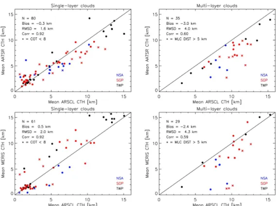
re-trievals. Biases are generally smallest for marine stratocu-mulus clouds: −0.28, 0.41 µm and −0.18 g m−2 for cloud optical thickness, effective radius and cloud water path, re-spectively. This is also true for the root-mean-square devia-tion. Furthermore, both cloud top height products are com-pared to cloud top heights derived from ground-based cloud radars located at several Atmospheric Radiation Measure-ment (ARM) sites. FAME-C mostly shows an underestima-tion of cloud top heights when compared to radar observa-tions. The lowest bias of−0.3 km is found for AATSR cloud top heights for single-layer clouds, while the highest bias of −3.0 km is found for AATSR cloud top heights for multi-layer clouds. Variability is low for MERIS cloud top heights for low-level clouds, and high for MERIS cloud top heights for mid-level and high-level single-layer clouds, as well as for both AATSR and MERIS cloud top heights for multilayer clouds.
1 Introduction
the largest uncertainty to the total radiative forcing estimate (IPCC, 2013).
Accurate observations of cloud properties on a global scale are needed for climate model development and evaluation, as well as for climate research. Satellite observations provide these global and long-term cloud observations. From obser-vations in the visible, near-infrared and thermal infrared parts of the electromagnetic spectrum, cloud macrophysical prop-erties, such as cloud amount and cloud top height – as well as cloud optical and microphysical properties such as cloud-top thermodynamic phase, cloud optical thickness and effective radius, which describes the cloud particle size distribution – can be retrieved.
A number of these types of cloud property retrievals and their accompanying global, long-term cloud data sets exist for a range of multispectral passive imagers on both polar-orbiting and geostationary satellites. Several of these data sets are included in the Global Energy and Water Cycle Ex-periment (GEWEX) Assessment of Global Cloud Datasets from Satellites (Stubenrauch et al., 2013). The objective of this assessment is to evaluate their overall quality. Partic-ipating cloud data sets include ATSR-GRAPE, based on observations from the Along-Track Scanning Radiometers (ATSRs) and the Advanced ATSR (AATSR) (Sayer et al., 2011); the International Satellite Cloud Climatology Project (Schiffer and Rossow, 1983), based on observations from im-agers on a set of satellites; the Pathfinder Atmospheres Ex-tended (PATMOS-x) (PATMOS-x, 2014), based on observa-tions from the Advanced Very High Resolution Radiometer (AVHRR) on the National Oceanic and Atmospheric Admin-istration (NOAA) satellites, as well as on the Meteorologi-cal Operation (MetOp) satellites of the European Organisa-tion for the ExploitaOrganisa-tion of Meteorological Satellites (EU-METSAT); and cloud products from the MODIS Science Team (NASA, 2014b) and MODIS CERES Science Team (NASA, 2014a), using observations from the Moderate Res-olution Imaging Spectroradiometer (MODIS) from the Na-tional Aeronautics and Space Administration (NASA) Earth Observing Satellites (EOS) Aqua and Terra. Intercompar-isons were performed on monthly mean, gridded cloud data sets. Results show that differences in average cloud proper-ties can arise due to, for example, retrieval filtering, ice-water cloud misidentification, assumptions on cloud particle shape and size distribution, and the set of spectral channels and an-cillary data used in the retrievals.
To assess the quality of retrieved cloud properties due to algorithm design itself, i.e., not accounting for instrument de-sign, the Cloud Retrieval Evaluation Workshop (CREW) was initiated by EUMETSAT (Roebeling et al., 2013). Level-2 cloud products derived from a set of well-established cloud property algorithms have been collected and intercompared for predefined days against observations from the active in-struments CALIOP (Cloud-Aerosol Lidar with Orthogonal Polarization) onboard CALIPSO (Cloud-Aerosol Lidar and Infrared Pathfinder Satellite Observations), CPR (Cloud
Pro-filing Radar) onboard CloudSat, and AMSR-E (Advanced Microwave Scanning Radiometer for EOS) onboard Aqua, all part of the A-train constellation. Participating cloud prop-erty algorithms include the CERES (Clouds and Earth’s Ra-diant Energy System) algorithm (Minnis et al., 2011); the DCOMP (Daytime Cloud Optical and Microphysical Prop-erties) algorithm (Walther and Heidinger, 2012), and the CPP (Cloud Physical Properties) algorithm (Roebeling et al., 2006). These kind of studies can reveal strengths and weak-nesses for different methods of cloud property retrievals (Hamann et al., 2014) and have shown that large differences can already arise due to different cloud detection methods. This will in turn also affect temporal and spatial averages of cloud properties for climate studies.
In the frame of the European Space Agency (ESA) Cli-mate Change Initiative (CCI) Cloud project (Hollmann et al., 2013), a 10-year daytime cloud climatology of synergis-tic AATSR and Medium Resolution Imaging Spectrometer (MERIS), both aboard the Environmental Satellite (Envisat), cloud observations is to be produced. The ultimate objective of the project is to provide long-term coherent cloud property data sets for climate research, taking advantage of the syn-ergy of different Earth observation missions. The FAME-C (Freie Universität Berlin AATSR MERIS Cloud) algorithm uses optimal estimation to retrieve a set of daytime cloud properties and their uncertainties on a pixel basis. MERIS and AATSR were not originally designed for cloud observa-tions, but together they provide a useful set of channels in the visible, near-infrared and thermal infrared wavelengths for cloud property retrieval. Furthermore, two independent cloud height products are retrieved: first, using AATSR brightness temperatures from two thermal infrared channels and, sec-ond, using the MERIS oxygen-A absorption channel. The follow-up instruments SLSTR (Sea and Land Surface Tem-perature Radiometer) and OLCI (Ocean Land Colour In-strument) onboard Sentinel-3 (ESA, 2014d), expected to be launched by mid-2015, will have very similar channel set-tings, making the FAME-C algorithm applicable to their ob-servations as well.
2 Observation data and preprocessing 2.1 Instruments
AATSR and MERIS are both imaging multispectral radiome-ters onboard the polar-orbiting satellite Envisat, which was launched in March 2002 and was in operational use until April 2012, providing a 10-year measurement data set. En-visat flies in a Sun-synchronous polar orbit around the Earth at a mean altitude of 800 km and a 98.5◦inclination. It has a repeat cycle of 35 days and the mean local solar time at de-scending node is 10:00. The MERIS instrument has 15 spec-tral channels, which are programmable in position and width within the solar spectral range (400 to 905 nm), and scans the Earth by means of a push-broom method. It has a hor-izontal resolution of just over 1 km at the subsatellite point and its field of view, resulting in a swath width of 1150 km, is covered using five identical optical cameras. AATSR has spectral channels in the visible part as well as in the near-infrared and thermal near-infrared part of the spectrum (channels at 0.55, 0.66, 0.87, 1.6, 3.7, 11 and 12 µm). It has a horizon-tal resolution of 1 km at subsatellite point and a swath width of 512 km. Due to its conical scanning method, it has a dual view of the Earth’s surface for all spectral channels. More details on both instruments can be found in Llewellyn-Jones et al. (2001), Rast et al. (1999) and ESA (2014c).
2.2 Collocation and cloud screening
Cloud property retrievals are performed for pixels identified as cloudy by a synergistic cloud mask, which is produced us-ing the cloud-screenus-ing module in the BEAM toolbox (Fom-ferra and Brockmann, 2005; ESA, 2014a). First, the AATSR observations are collocated with MERIS observations on the MERIS grid (reduced resolution mode, 1200 m×1000 m) using a nearest-neighbor technique. This grid was chosen be-cause of MERIS’s better geolocation. Then, a cloud screen-ing is performed by combinscreen-ing a set of neural networks op-timized for different cloudy situations and using all AATSR and MERIS channels. Finally, the produced synergy prod-uct contains all AATSR and MERIS channels as well as the newly produced cloud mask. It should be noted that the synergy product has a swath width of 493 pixels, which is less than the AATSR swath width of 512 pixels. This is re-lated to collocating the curved AATSR grid with the MERIS grid. Technical details on the collocation and cloud-screening method can be found in Gómez-Chova et al. (2008) and Gómez-Chova et al. (2010).
2.3 Drift and stray light correction
An improved long-term drift correction is applied to the AATSR reflectances for the visible and near-infrared chan-nels from the second reprocessing as described in Smith et al. (2008). For MERIS measurements, the third reprocessing has been used (ESA, 2011). Furthermore, an empirical stray
light correction was applied to the reflectance of the MERIS oxygen-A absorption channel (Lindstrot et al., 2010). For this correction, the spectral smile effect in the MERIS mea-surements (Bourg et al., 2008), which is the variation of the channel center wavelength along the field of view, as well as the amount of stray light in the MERIS oxygen-A absorption channel, was determined.
3 Forward model
3.1 Cloud optical and microphysical properties
The retrieval of the cloud optical and microphysical prop-erties cloud optical thickness (COT,τ) and effective radius (REF,reff) for water and ice clouds, and subsequently also
cloud water path (CWP), is based on the DCOMP algorithm and largely follows the approach as described in Walther and Heidinger (2012). The COT–REF pair is retrieved using si-multaneous measurements of the AATSR 0.66 and 1.6 µm channels. It is based on the assumption that the reflectance in the visible (VIS) mainly depends on COT due to conser-vative scattering, while the reflectance in the near-infrared (NIR) mainly depends on the cloud droplet size distribution due to weak absorption. This method is based on work by Nakajima and King (1990) and has since been used in a num-ber of cloud property retrievals (e.g., Nakajima and Nakajma, 1995; Roebeling et al., 2006; Walther and Heidinger, 2012). Lookup tables (LUTs) for both water and ice clouds con-sisting of cloud reflectances have been created with simula-tions from the radiative transfer model MOMO (Matrix Op-erator Model). MOMO was developed at the Freie Univer-sität Berlin (Fell and Fischer, 2001; Hollstein and Fischer, 2012) and allows for simulations of radiative transfer in a plane-parallel homogeneous scattering medium with any ver-tical resolution. The cloud reflectance,Rc,λ, at wavelengthλ (wavelength dependency will not be used in the text from now on) is given by
Rc,λ=
π·Lc,λ(θ0, θ, φ, τ, reff)
cos(θ0)·F0,λ(θ0)
, (1)
whereLc is the radiance reflected by the cloud and F0 is
the incoming solar irradiance at the top of the atmosphere. The radianceLcis a function of solar zenith angleθ0,
view-ing zenith angleθ, and relative azimuth angleφ, as well as cloud optical thickness and effective radius. The simulations have been performed assuming a homogeneous cloud and no contribution from the atmosphere as well as the surface, i.e., no gaseous absorption, Rayleigh scattering and aerosol ex-tinction, and zero surface albedo. Then, the reflectance at the cloud topR′tocwhen including a Lambertian reflecting sur-face is computed as follows:
Rtoc′ ,λ=Rc,λ+
αλ·tc,λ(θ0, τ, reff)·tc,λ(θ, τ, reff)
1−αλ·Sλ(τ, reff)
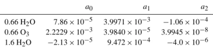
Table 1. Atmospheric correction coefficients for AATSR 0.66 and 1.6 µm channels.
a0 a1 a2
0.66 H2O 7.86×10⁻⁵ 3.9971×10⁻³ −1.06×10⁻⁴ 0.66 O3 2.2229×10⁻³ 3.9840×10⁻⁵ 3.9945×10⁻⁸ 1.6 H2O −2.13×10⁻⁵ 9.472×10⁻⁴ −4.0×10⁻⁶
whereαis the surface albedo;tc(θ0)andtc(θ )are the cloud
transmittance in the downward and upward directions, re-spectively; andSis the spherical albedo.
To compare the measured reflectances at the top of the at-mosphere to the forward model results, which are simulated reflectances without consideration of atmospheric extinction processes, the measured reflectances are corrected for at-mospheric extinction of radiation due to gaseous absorption and Rayleigh scattering. Other sources of extinction, e.g., aerosols, are not considered. The top-of-cloud reflectance,
Rtoc, is computed from the measured top-of-atmosphere
re-flectance,Rtoa, as follows:
Rtoc,λ=
Rtoa,λ−RRS,λ(θ0, θ, φ, τ, reff, pc)
ta,λ(θ, θ0)
, (3)
where RRS is the back-scattered signal due to single
scat-tering events above the cloud (here only Rayleigh scatter-ing in the visible channel is taken into account) and ta is
the two-way atmospheric transmittance above the cloud. The Rayleigh scattering correction is based on Wang and King (1997) and is only performed in the VIS channel. Next to the viewing geometry, it depends on cloud albedoαc, which in
turn depends on COT and REF, and Rayleigh optical thick-ness from cloud top to the top of the atmosphere, τr. The
Rayleigh optical thickness is determined assuming a total column Rayleigh optical thickness of 0.044 at surface pres-sure 1013 hPa (Wang and King, 1997) and scaling it by an estimated cloud top pressurepc. The atmospheric
trans-mittance above the cloud is determined considering absorp-tion by water vapor (total column water vapor above cloud) and ozone (total ozone in Dobson units) in the VIS chan-nel and only absorption by water vapor in the NIR chanchan-nel. A quadratic relationship, and its accompanying coefficients,
ai, between the amount of absorber gasM (here water va-por or ozone) above cloud and the gas transmittance,ta, also
depending on air mass factor (AMF), is determined using a number of MODTRAN simulations. The gas transmission is computed as follows:
ta,M,λ=e−AMF·[a0,λ+a1,λM 1+a
2,λM2]. (4)
The atmospheric correction coefficients for the AATSR channels are listed in Table 1.
To account for atmospheric absorption below the cloud, the surface albedo in Eq. (2) is adjusted to a so-called vir-tual surface albedo αv by multiplying the surface albedo
with the atmospheric transmittance below the cloud. The atmospheric transmittance below the cloud is computed in the same manner as the atmospheric transmittance above the cloud. For the computation of the atmospheric transmit-tance below the cloud, a diffuse radiation field below the cloud is assumed, which means that an air mass factor of 2 is used. Rayleigh scattering is not considered below the cloud. The altitude of the cloud is roughly estimated using the AATSR 11 µm brightness temperature and atmospheric temperature and pressure profiles from model data (described in Sect. 3.3). The full forward model looks as follows:
Rtoc,v,λ=Rc,λ+
αv,λ·tc,λ(θ0, τ, reff)·tc,λ(θ, τ, reff)
1−αv,λ·Sλ(τ, reff)
. (5) Cloud reflectance, cloud transmittance, spherical albedo and cloud albedo have all been computed for both water and ice clouds. For radiative transfer simulations with wa-ter clouds, Mie calculations (Wiscombe, 1980) have been performed beforehand to compute scattering phase functions as well as single-scattering albedo and normalized extinction coefficient, which serve as input to MOMO. In the Mie cal-culations a modified gamma-Hansen cloud droplet size dis-tributionn(r)is assumed (Hansen and Travis, 1974), where the mode radius equals the effective radius (Hansen and Hov-enier, 1974):
reff= R∞
0 r3n(r)dr R∞
0 r2n(r)dr
, (6)
whereris the cloud droplet radius. A value of 0.1 for the ef-fective variance is assumed for this droplet size distribution (Minnis et al., 1998). For ice clouds, single-scattering prop-erties described in Baum et al. (2005) have been used in the radiative transfer simulations. In the LUTs the COT and REF (inµ) range in log10space from−0.6 to 2.2 in 29 steps and 0.4 to 2.0 in 9 steps, respectively.
From theτ−reffpair the liquid water path (LWP) for
wa-ter clouds and the ice wawa-ter path (IWP) for ice clouds are determined, assuming a plane-parallel homogeneous cloud, as follows:
CWP=2
3·τ·reff·ρ, (7)
whereρis the density of liquid or frozen water (g m−3). For optically thin ice clouds the following equation is used to compute ice water path, which is based on observations of mid-latitude thin ice clouds (Heymsfield et al., 2003):
IWP=τ·
g
0
reff
·
1+g1
g0
−1
, (8)
whereg0andg1are constants with values 0.01256 and 0.725,
respectively.
AATSR 11 µm channel, combined with a cirrus detection us-ing the brightness temperature difference BT11–BT12
tech-nique (Saunders and Kriebel, 1988) and a maximum re-flectance in the visible of 0.25. At 261 K the difference in equilibrium water vapor pressure with respect to ice and wa-ter is largest, favoring the growth of ice crystals over super-cooled water droplets for temperatures below 261 K (Prup-pacher and Klett, 1997). For the cirrus detection a dynamic clear-sky brightness temperature difference threshold, de-pending on atmospheric moisture and surface temperature, is used. The clear-sky radiative transfer simulations have been performed with MOMO using a set of standard atmospheric profiles as input taken from McClatchey et al. (1972). From visual inspection of retrieved cloudy scenes the method also often appears to detect cloud edges.
3.2 Cloud top heights
Two cloud top height products are retrieved within FAME-C. First, the cloud top temperature (CTT) using AATSR bright-ness temperatures is retrieved. Second, the cloud top pres-sure (CTP) is retrieved using the ratio of the MERIS oxygen-A absorption channel over a nearby window channel. Both cloud top height retrievals are then converted into cloud top heights (in km) using the input atmospheric profiles. 3.2.1 AATSR cloud top temperature
The cloud top temperature is retrieved using measurements at the 11 µm channel and the 12 µm channel, at which the extinction coefficient of water is larger. The forward model, assuming a plane-parallel atmosphere, consists of three parts contributing to the top-of-atmosphere radiation in cloudy sit-uations: cloud, surface and atmosphere. The contribution of the cloudIc,λis given as follows:
Ic,λ=ǫc(τ, θ )·B(Tct, λ)·tct→1,λ(θ ), (9) whereǫcis the cloud emissivity;B(Tc)is the Planck function
at the temperature of the cloud topTct, assuming the cloud to
be in thermal equilibrium with the surrounding air; andtct→1
is the atmospheric transmittance from the cloud top to the top of atmosphere. The cloud emissivity is computed as follows:
ǫc=1−exp −τ
ir
cosθ
, (10)
whereτiris the cloud optical thickness in the thermal
in-frared. Here, no multiple scattering is assumed and the ther-mal infrared cloud optical thickness is computed from the visible cloud optical thicknessτvis, which is taken from the
cloud optical and microphysical property retrieval. The sim-ple relationshipτir=0.5·τvisis used, which is about true for
large water and ice particles (Minnis et al., 1993). The contribution of the surfaceIs,λis given as follows:
Is,λ=ǫs,λ·B(Ts, λ)·ta,λ(θ )·tc(θ ), (11)
whereǫsis the surface emissivity,B(Ts)is the Planck
func-tion at the surface temperatureTs,ta is the transmittance of
the atmosphere, andtcis the transmittance of the cloud. The
cloud transmittance is computed from the cloud emissivity withtc=1−ǫc. The contribution of the atmosphere at the
top of atmosphereIa,λis given as follows:
Ia,λ= (12)
1 Z
ts,λ
B(Ta, λ)dtλ+1−ǫs,λ·ts,λ(θ )2·
1 Z
ts,λ
B(Ta, λ)
tλ(θ )2 dtλ,
wherets is the total transmittance from surface to the top
of the atmosphere, andB(Ta)is the Planck function at the
atmospheric temperatureTa of the level with transmittance
t. The second term in the equation is of second order and arises from downward radiance reflected upward at the sur-face. For cloudy layers, the atmospheric transmittanceta,j of layerjis multiplied by the cloud transmittancetc,jto get the total transmittancetat layerj. The vertical extension of the cloud and the vertical distribution of cloud layer transmit-tance/emissivity values are based on vertical cloud profiles explained in Sect. 3.2.2. For atmospheric levels below the cloud the atmospheric transmittances are multiplied by the total cloud transmittancetc. For very thick clouds with cloud
emissivities equal to 1, the surface and atmospheric layers below the cloud do not contribute to the top-of-atmosphere radiance.
The fast radiative transfer model RTTOV version 9.3 (Saunders et al., 2010; METOffice, 2014) is used to simu-late the clear-sky transmission for both AATSR IR channels at a given number of atmospheric levels. Given as input into RTTOV are atmospheric profiles of temperature, water vapor and ozone concentrations, as well as the temperature, wa-ter vapor concentration and pressure near the surface. Both the atmospheric profiles and surface properties are obtained from ERA-Interim reanalysis and forecasts (to be described in Sect. 3.3). At the time of development the optical parame-ter file for ATSR on ERS (version 7) was used. This will lead to a small error in the simulated AATSR brightness tempera-tures due to slightly different spectral response functions for the IR channels of the two instrument.
3.2.2 MERIS cloud top pressure
The cloud top pressure (CTP) is retrieved using the radi-ance ratio of the MERIS oxygen-A absorption channel 11 at around 760 nm (L11) and a nearby window channel 10
at around 753 nm (L10), representing an apparent
transmit-tance:
to2= L11
L10
. (13)
through the atmosphere. In cloudy situations this average photon path length mainly depends on cloud top pressure.
MOMO radiative transfer simulations have been per-formed to create a LUT in which the ratio depends on cloud top pressure as well as cloud optical thickness, view-ing geometry, surface pressure and the MERIS channel 11 center wavelength. A US standard atmosphere (McClatchey et al., 1972) is assumed in the simulations. Thek-distribution method (Bennartz and Fischer, 2000; Doppler et al., 2014) is used to compute the absorption coefficients of the atmo-spheric gases. Information on the position and width of ab-sorption lines is taken from the HITRAN database (Roth-man et al., 2009). The CTP ranges from 100 to 1000 hPa in the LUT. For cloud layers below 440 hPa, ice crystals are as-sumed with a fixed effective radius of 40 µm; otherwise water droplets are assumed with a fixed effective radius of 10 µm. A previous sensitivity study (Preusker and Lindstrot, 2009) has shown that the cloud microphysical properties and the temperature profile account for errors of less than 10 and 20 hPa, respectively, in the MERIS-CTP retrieval and are much smaller than other error sources such as the presence of mul-tilayer clouds and unknown subpixel cloud fraction. For CTP retrievals above high land surfaces, the surface pressure has to be taken into account to prevent underestimation of CTP. For retrievals above oceans a surface pressure of 1013 hPa is assumed. To account for the spectral smile effect in the MERIS measurements, radiative transfer simulations are per-formed for varying center wavelengths in the oxygen-A ab-sorption channel.
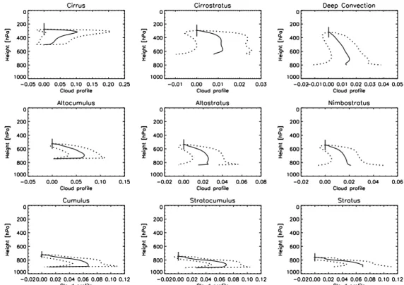
Due to in-cloud scattering, the average photon path length is increased. This increase depends on the vertical extinc-tion profile of the cloud. To derive “realistic” cloud vertical extinction profiles for nine cloud types based on the ISCCP cloud classification (ISCCP), 1 year (2010) of layer optical thicknesses as provided by the CloudSat database is used as described in Henken et al. (2013). The geometrical thickness of each cloud type, i.e., the number of adjacent cloud layers with a thickness of 20 hPa, is taken constant and based on an empirical analysis of a number of CloudSat scenes. The re-sulting averaged and normalized vertical extinction profiles are shown in Fig. 1. For most cloud types it can be seen that lower cloud layers tend to have higher extinction values than upper cloud layers. In the radiative transfer simulations of the MERIS channels 10 and 11 radiances, the cloud is di-vided into a number of cloud layers, each with a thickness of 20 hPa. The appropriate extinction profile, and thus the extinction of each cloud layer, is selected according to the ISCCP cloud classification. This means that the layer cloud optical thickness is different for each cloud layer, while it would be taken constant for all cloud layers when assum-ing a vertically homogeneous cloud. The total cloud optical thickness is taken from the cloud optical and microphysical property retrieval.
3.3 Auxiliary data
A set of auxiliary data is needed within the FAME-C al-gorithm. For the atmospheric correction in the cloud opti-cal and microphysiopti-cal property retrieval, atmospheric pro-files from ERA-Interim reanalyses (00+00 and 12+00 UTC) and forecasts (00:00 +6 h and 12:00 UTC +06) are used. They are linearly interpolated in time, but kept on the ERA-Interim spatial resolution of 1.125◦. The interpolated atmo-spheric profiles and surface properties also serve as input in the RTTOV clear-sky simulations. Furthermore, the IR land surface emissivities are taken from the UW-Madison Base-line Fit Emissivity Database (Seemann et al., 2008). The cloud optical and microphysical property retrieval uses the MODIS 16-day composite white-sky surface albedo prod-uct (MCD43C3; NASA Land Processes Distributed Active Archive Center (LP DAAC)) on a 0.05◦spatial grid as input,
while the MERIS-CTP retrieval uses the 2005 monthly mean MERIS-derived land surface albedo product (Muller et al., 2007). To account for pixels that might contain snow-covered surfaces, the MODIS monthly mean snow cover product (MYD10CM; Hall and Riggs., 2006) on a spatial 0.05◦grid is used. Sea ice cover is taken from ERA-Interim. For wa-ter surfaces and surfaces containing snow or ice fractions of more than 50 %, fixed surface albedo and surface emissiv-ity values are taken from narrowband mean surface albedo (Chen et al., 2006) and surface emissivity (Chen et al., 2003) for water and snow/ice surfaces derived from MODIS-Terra data. The surface pressure that serves as input in the MERIS-CTP retrieval is estimated on a pixel basis from the MERIS surface height provided as meta-data in the AATSR–MERIS synergy product. The synergy product also provides for a pixel-based land–sea mask.
4 Retrieval scheme
Figure 1. Normalized mean cloud vertical extinction profiles (solid line) for nine cloud types based on the ISCCP cloud classification. The standard deviation of extinction is shown by the dotted line, and the standard deviation of the cloud top pressure is shown by the error bar.
4.1 Inversion technique
The retrieval of the cloud parameters is based on the optimal estimation method. This inversion technique allows for the combined use of an a priori estimate of the most likely so-lution,xa, and the measurements given in the measurement
vector yto maximize the probability of the retrieved cloud parameters given in the state vector x. The cloud parame-ters, their a priori values with uncertainties, and measure-ments with uncertainties are listed in Table 2. Bothxa and yare weighted by their uncertainty estimates given in the er-ror covariance matrices Saand Sy, respectively. In short, the
inversion technique aims to minimize the retrieval cost func-tionJ given as
J (x)=y−F (x,b)TS−1y y−F (x,b) (14) +[x−xa]TS−1a [x−xa],
whereF (x,b)is the output of the forward model for statex and background stateb. The forward model parameters and their uncertainties are listed in Table 3. The background state vector, or forward model parameter vector, includes param-eters that are not retrieved but do affect the retrieval. Due to nonlinearity in the forward model the minimization is per-formed within an iterative process. Here, the Gauss–Newton method is used. A first guess, also listed in Table 3, is used to start the iteration. The iteration is terminated when the differ-ence between the error-weighted length of two consecutive
state vectors is 1 order of magnitude smaller than the length of the state vector, or the maximum number of allowed iter-ations has been reached. The error covariance matrix of the retrieved state Sxcan be computed as follows:
Sx=hKTS−1y K+S−1a i
−1
, (15)
where K is the Jacobian matrix describing the sensitivity of
F to changes in state parameters. This way, the pixel-based retrievals are accompanied by pixel-based uncertainties.
It has to be noted that the optimal estimation method is built on the assumption that the state parameters and their er-rors, as well as the observation erer-rors, show a Gaussian dis-tribution, and the iteration method assumes thatF changes linearly with small changes in the state parameters. To meet these assumptions, theτ−reffpair is retrieved in a
logarithm-based space. An in-depth mathematical description of opti-mal estimation can be found in Rodgers (2000).
Figure 3 shows an example of the cloud mask and retrieved cloud parameters for a cloudy scene above Germany. 4.2 Uncertainty estimates
The reliability of the error covariance matrix of the retrieved state depends on the reliability of the characterization of Sy and Sa, i.e., on the estimated uncertainties in the
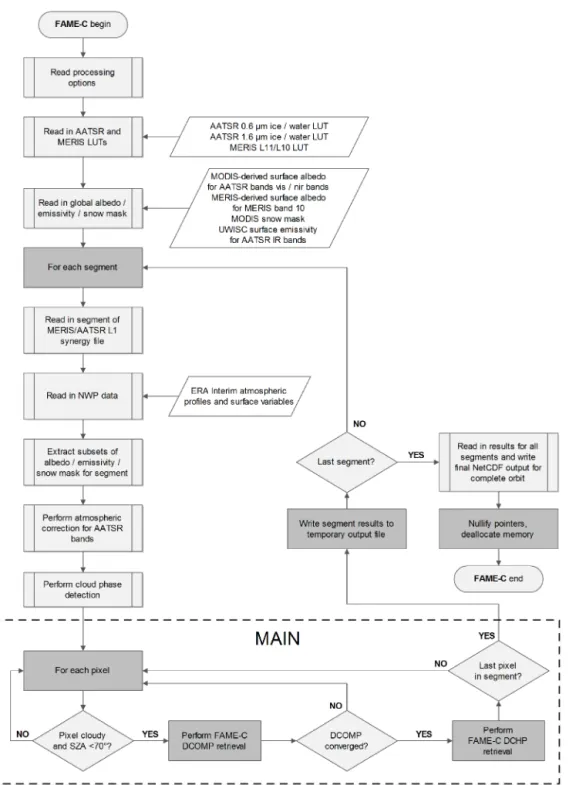
Figure 2. FAME-C algorithm flowchart with two main retrieval steps DCOMP (Daytime Cloud Optical and Microphysical Properties) and DCHP (Daytime Cloud top Height Properties) and input and output data.
parameters in the forward model, can be added to the mea-surement uncertainties to form a combined meamea-surement er-ror covariance matrix Sǫas follows:
Sǫ=Sy+KBSBKTB, (16)
where SB is the forward model error covariance matrix and KBis the Jacobian matrix, which describes the sensitivity of
F to changes in the forward model parameters.
possi-Table 2. Listed are the variables in the state vector x, the measurements in the measurement vectory (R: reflectance; BT: brightness temperature;L: radiance) and their uncertaintiesyunc, and the a priori values in the a priori state vectorxaand their uncertaintiesxa_unc,
used in the Daytime Cloud Optical and Microphysical Cloud Properties retrieval (DCOMP) and both Daytime Cloud Top Height properties retrievals for AATSR measurements (DCHP-A), and MERIS measurements (DCHP-M). Here, wat and ice are the water and both Daytime Cloud Top Height Properties retrieval for ice cloud phases, respectively. Note thatxaandxa_uncare in log10space in DCOMP.
Algorithm x, (symbol) [unit] y:yunc xa:xa_unc
DCOMP COT (τ) R0.66 µm: 4 % wat=1.0: 2.0, ice=1.0: 2.0 REF (reff) [ µm] R1.6 µm: 4 % wat=1.2: 2.0, ice=1.6: 2.0
DCHP-A CTT [K] BT 11 µm: 0.1 K wat=280 K: 40 K, ice=250 K: 40 K BT 12 µm: 0.1 K
DCHP-M CTP [hPa] L761 nm/L753nm: 0.004 % wat=800 hPa: 300 hPa, ice=300 hPa: 300 hPa
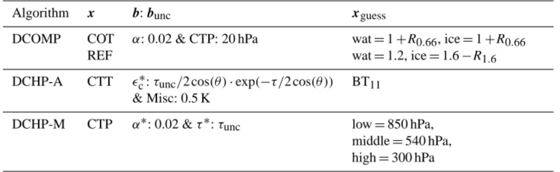
Table 3. Listed are the forward model parametersband their uncertaintiesbuncas well as the first guessxguessused in the Daytime Cloud
Optical and Microphysical Cloud Properties (DCOMP) retrieval and both the Daytime Cloud top Height Properties for AATSR (DCHP-A) and MERIS measurements (DCHP-M). The cloud optical thickness (COT, τ) uncertainty,τunc, is taken from the DCOMP results. Misc
stands for miscellaneous and is an estimated forward model parameter uncertainty arising from differences in spectral response function of ATSR-2 (assumed in clear-sky RTTOV simulations) and AATSR, as well as tabular integration. In the cloud top pressure (CTP) retrieval, different first guesses are used for low (>680 hPa), middle (>400 and<680 hPa) and high (<400 hPa) clouds. To estimate the cloud height level, the previously retrieved cloud top temperature is converted to cloud top pressure using the ERA-Interim temperature profile. Here,α
is surface albedo;ǫcis cloud emissivity; wat and ice are the water and ice cloud phases, respectively;R0.66andR1.6are the reflectances in
the AATSR 0.66 and 1.6 µm channels, respectively; and BT11is the brightness temperature in the AATSR 11 µm channel. Note thatxguess
is in log10space in DCOMP.∗Only performed for pixels withτ <8.
Algorithm x b:bunc xguess
DCOMP COT α: 0.02 & CTP: 20 hPa wat=1+R0.66, ice=1+R0.66
REF wat=1.2, ice=1.6−R1.6
DCHP-A CTT ǫc∗:τunc/2 cos(θ )·exp(−τ/2 cos(θ )) BT11
& Misc: 0.5 K
DCHP-M CTP α∗: 0.02 &τ∗:τunc low=850 hPa,
middle=540 hPa, high=300 hPa
ble solutionsx. Estimated uncertainties in the measurements (based on ESA (2014b) for AATSR) as well as for a set of forward model parameters are listed in Tables 2 and 3, re-spectively. For certain pixels that have reached convergence, we take into account the uncertainties due to the rather sim-ple cloud phase discrimination. This is realized by adding the difference in forward model values between the water cloud and ice cloud, keeping everything else constant, to the measurement error covariance matrix. This is done for pixels with 11 µm brightness temperatures between 245 and 273 K and where the reflectance pair 0.66–1.6 µm lies within both the water and ice cloud LUT. Figure 4 shows the at-mospheric corrected 0.66 and 1.6 µm reflectances for cloudy pixels from the scene as shown in Fig. 3 together with the AATSR LUT reflectances for a mean viewing geometry and surface albedo, as a function of cloud optical thickness and effective radius and for both water and ice clouds. Shown in green are the cloudy pixels with an uncertain retrieved cloud phase located in the overlapping area of the water and ice
LUT. According to our forward models in this area we can have both large water droplets and small ice crystals or a mix of both.
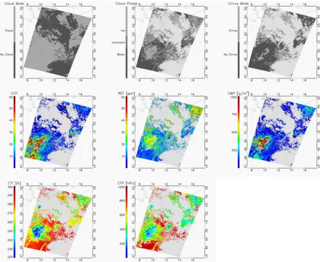
Figure 3. Example of the FAME-C cloud mask; cloud phase mask; cirrus mask; and retrieved cloud optical, microphysical and macrophysical properties for a synergy AATSR–MERIS orbit segment above Germany on 21 July 2007.
emissivity and COT are propagated to uncertainties in CTT and CTP, respectively. In general, the relative uncertainty is highest for pixels with uncertain cloud phase and lowest for water cloud pixels.
Uncertainties in ERA-Interim atmospheric profiles are ne-glected. Also, uncertainties in the radiative transfer simu-lations and chosen cloud microphysical models, as well as those due to interpolations in the LUTs, are not considered at present.
Last, the forward model assumes fully cloudy pixels with plane-parallel clouds consisting of either water droplets or ice crystals. The impact of subpixel clouds, three-dimensional effects (e.g., cloud shadows), multilayer cloud situations and mixed-phase clouds needs to be studied in the future for an improved uncertainty estimate budget.
5 Verification
To verify the performance of the FAME-C cloud properties, two comparisons were performed for selected areas and for the years 2007–2009.
5.1 Comparison to MODIS-Terra level-2 cloud optical and microphysical properties
The comparison of the FAME-C level-2 cloud optical and microphysical properties to the MODIS-Terra level-2 cloud optical and microphysical properties (MOD06 collection-5 cloud products) is performed for four selected regions as shown in Fig. 5. For each region, all available orbit seg-ments of both Envisat and Terra are collected. Overpasses of the satellites Terra and Envisat do not necessarily occur on the same days. Therefore, no pixel-based comparison is possible. From all selected cloudy pixels within the region and within 1 month, monthly means and standard deviations are produced for each of the cloud optical and microphysical properties.
Figure 4. AATSR atmospheric corrected reflectance in the visible and near infrared (dots) for water, ice, uncertain and cirrus pixels from the scene shown in Fig. 3. The two grids represent the forward-modeled AATSR reflectances for water (red) and ice (blue) clouds, assuming mean viewing geometry and surface albedo values for the scene.
for the MODIS cloud optical and microphysical properties cloudy pixels with a general assessment set to Useful accord-ing to the quality flag (quality assurance at 1×1 resolution) are selected. For FAME-C, successfully retrieved cloudy pix-els, as defined in Sect. 4.2, are selected.
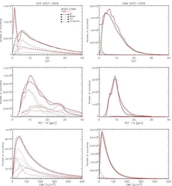
Figure 7 shows the frequency distribution of COT, REF and CWP for all retrieved cloudy pixels in the time period 2007–2009 for both FAME-C and MODIS-Terra for two se-lected regions, GER and NAM, as presented in Fig. 5. Also, a distinction in cloud phase is made. Generally, the overall dis-tributions agree well with similar shapes and peaks located around similar values. This is expected, especially for NAM, since one cloud regime, marine stratocumulus clouds, domi-nates this region. Differences become larger when only con-sidering one specific cloud phase. For NAM both FAME-C and MODIS-Terra agree that almost all pixels consist of the water cloud phase. For both regions, FAME-C has a larger number of pixels with uncertain cloud phase. A major dif-ference is the sharp peak at low COT values for FAME-C, mainly consisting of ice phase. We assume this to be pix-els misidentified as cirrus clouds through the cirrus detec-tion method, and the peak vanishes when these pixels are not considered. Consequently, the peak CWP is shifted towards lower values for FAME-C. The FAME-C REF values agree very well with the MODIS-Terra REF values for NAM. In GER, the second peak in the MODIS-Terra REF arising from the ice cloud phase is not visible in FAME-C REF.
Table 4 lists, for each region and cloud property, the bias and root-mean-square deviation (RMSD) computed from the monthly means in the 3-year time period. They have been computed for all successfully retrieved cloudy pixels (All), and separately for cloudy pixels identified as water cloud
Figure 5. Map showing four regions where level-2-based com-parisons between FAME-C and MODIS-Terra cloud properties are conducted for the years 2007–2009. SAO: southern Atlantic Ocean; NAM: coast of Namibia; CAF: central Africa; GER: Germany.
(Wat), ice cloud (Ice) and with uncertain cloud phase (Unc). The cloud fraction here is defined as the cloud fraction which only considers successfully retrieved cloudy pixels, so those pixels contributing to the statistics of the cloud optical and microphysical properties. The cloud phase fractions are con-sidered relative to this overall retrieval cloud fraction. It should be emphasized that the cloud fractions and the frac-tion of clouds with a specific phase, in particular uncertain cloud phase, can be quite different for FAME-C and MODIS-Terra, and consequently this will affect the statistics of the other cloud properties.
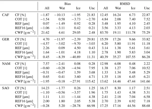
Table 4. Results of the comparison with monthly mean MODIS-Terra cloud optical and microphysical properties for four regions as presented in Fig. 5. Performed for all successfully retrieved cloudy pixels (All), and separately for water cloud pixels (Wat), ice cloud pixels (Ice), and cloudy pixels with uncertain phase (Unc), for cloud properties cloud fraction (CF), cloud optical thickness (COT), effective radius (REF) and cloud water path (CWP). REF16 is the MODIS-Terra effective radius retrieved using the 1.6 µm channel. RMSD is root-mean-square deviation.
Bias RMSD
All Wat Ice Unc All Wat Ice Unc
CAF CF [%] −1.87 −10.13 −1.95 21.83 12.45 16.24 6.73 22.87 COT [1] −1.54 0.58 −3.73 −2.70 4.84 2.08 7.40 7.52 REF [µm] 0.07 −1.49 0.92 0.28 3.48 1.95 4.10 2.45 REF16 [µm] −1.06 −3.11 0.42 0.21 3.56 3.33 4.13 2.03 CWP [g m−2] 21.62 4.61 29.05 2.48 83.70 19.11 111.78 75.29
GER CF [%] 4.70 −11.97 −2.39 29.81 15.59 17.26 9.66 33.82 COT [1] −4.57 −3.02 −9.70 −3.03 6.20 5.80 11.91 11.18 REF [µm] 2.26 0.09 4.50 0.43 3.14 1.38 5.61 3.61 REF16 [µm] 1.64 −1.01 4.18 1.10 2.78 1.90 5.83 3.04 CWP [g m−2] 0.45 −8.39 −40.89 11.31 40.39 35.27 107.55 86.28
NAM CF [%] 7.57 −2.41 0.08 0.28 12.98 6.08 0.48 2.22 COT [1] −0.60 −0.28 −4.94 7.95 1.38 1.27 7.06 10.52 REF [µm] −0.31 −0.47 1.59 3.68 1.33 1.34 5.48 5.29 REF16 [µm] 0.65 0.41 3.60 4.71 1.35 1.18 6.45 6.21 CWP [g m−2] −1.95 −0.18 −27.91 115.42 13.62 14.46 47.44 141.66
SAO CF [%] 14.23 −1.77 0.26 1.25 16.17 8.30 1.17 2.51 COT [1] −1.10 −0.56 −3.57 1.96 1.75 1.43 4.38 5.31 REF [µm] 1.11 1.11 −1.44 4.38 2.41 2.18 7.04 6.58 REF16 [µm] 2.00 1.80 2.05 5.38 2.70 2.39 6.92 7.18 CWP [g m−2] −0.28 5.20 −28.78 66.98 17.25 17.16 44.56 88.68
negative bias for GER. This can be attributed to a large num-ber of optically thin ice clouds retrieved with FAME-C, but not with MODIS-Terra. First inspections have revealed that this is due to misidentified cirrus clouds, which, through vi-sual inspection, appear to be mainly cloud edges. Neglecting those pixels reduces the overall COT, REF and REF16 biases to−1.92, 1.01 and 0.45 µm, respectively, but increases the CWP bias to 25.20 g m−2.
The bias between the REF where both FAME-C and MODIS-Terra-retrieved REF using the 1.6 µm channel (REF16) is not necessarily smaller than the bias when MODIS-Terra uses the 2.1 µm channel (REF). The NAM re-gion is dominated by marine stratocumulus clouds, which are relatively horizontally homogeneous and sub-adiabatic (e.g., Pawlowska and Brenguier, 2000). An adiabatic cloud shows an increasing REF with height. The penetration depth at 1.6 µm is larger than at 2.1 µm and would result in a lower retrieved effective radius assuming an adiabatic cloud. Therefore, in that case a negative bias would be expected when comparing the FAME-C REF retrieved using 1.6 µm and MODIS-Terra REF using 2.1 µm. When comparing both REF retrievals at 1.6 µm, a slight positive bias is found. Re-trievals of REF using different near-infrared channels can, however, also be affected differently by, for example, 3-D
radiative effects (e.g., Zhang et al., 2012), which makes in-terpretation of small differences difficult. The CWP bias is largest for the CAF region. However, this is also the region where deep convection takes place, which can result in very high CWP values. Mostly, biases are largest for pixels with uncertain cloud phase followed by the ice cloud phase. This is also true for the RMSD.
It should be noted that the Terra satellite flies in a Sun-synchronous near-polar orbit with a mean local solar time of 10:30. at descending node, which is half an hour later than the Envisat satellite. Slightly shifted observation times as well as different viewing geometry can also contribute to differences in mean cloud properties.
5.2 Comparison to cloud top heights derived from ground-based radar observations
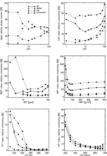
Figure 6. Histograms of the mean relative phase fraction and mean relative uncertainty estimates for FAME-C cloud properties cloud optical thickness (COT), effective radius (REF), cloud water path (CWP), cloud top temperature (CTT) and cloud top pressure (CTP) for all successfully retrieved cloudy pixels (converged and cost
<20) for orbit segments covering the region in Germany between lat. 9 and 14◦and long. 49 and 54◦(presented in Fig. 5 as GER) for the years 2007–2009. Results are shown separately for the three cloud phases – water, ice and uncertain – and for all cloudy pixels.
(MMCR) and Micropulse Lidar (MPL) data (Clothiaux et al., 2000). The cloud boundaries are provided at a vertical reso-lution of 45 m, a temporal resoreso-lution of 10 s, and for up to 10 cloud layers.
For the comparison the dates and times of the Envisat over-passes at each ARM site are determined. For each overpass, the mean and standard deviation of both FAME-C cloud top height products are computed for a 9×9 pixel box centered around the pixel that matches best with the ARM site latitude and longitude values. Before doing so, parallax correction was performed for cloudy pixels. The mean ARSCL cloud top height is computed from cloud top heights within a 5 min period centered at the Envisat overpass time. Here, the AR-SCL cloud top height is defined as the height of the highest cloud layer. The cases were selected based on the following
three criteria. First, at least 75 % of the pixels in the FAME-C 9×9 pixel box show a successful cloud top height re-trieval for either AATSR or MERIS measurements. Second, for all time steps within the 5 min period, an ARSCL cloud top height is determined by the MMCR. Third, the standard deviation of both FAME-C and ARSCL cloud top heights is less than 1 km. This results in 115 cases for AATSR and 90 for MERIS. We assume this difference in cases between both FAME-C cloud top height retrievals to be partly related to the fact that at the moment the MERIS cloud top pressure retrieval tends to fail more often than the AATSR cloud top temperature retrieval. This is related to the use of the differ-ent cloud vertical extinction profiles derived from CloudSat data for different cloud types in the radiative transfer simu-lations used to create the MERIS LUT and leads to jumps in the LUT at the cloud type transitions. It is envisaged that this issue will be dealt with in future versions of FAME-C.
Figure 8 shows the comparison of AATSR and MERIS cloud top heights to the ARSCL cloud top heights for single-layer and multisingle-layer cloud cases. Single-single-layer clouds are de-fined as cases where at least 80 % of the radar observations in the 5 min time period only show one cloud layer. Multilayer cloud cases are defined as cases in the ARSCL product where at least two cloud layers exist with a minimum distance of 1 km between the cloud top height of the lower cloud layer and the cloud base height of the upper cloud layer, for at least 80 % of the radar observations in the 5 min time period.
For single-layer clouds there is an overall small negative bias of−0.3 km found between AATSR and ARSCL cloud top heights. Taking into account only the single-layer cloud cases with ARSCL cloud top heights larger than 3.5 km, i.e., the mid-level and high-level clouds, the bias is−1.1 km with an RMSD of 1.9 km. This negative bias falls within the ex-pected range of a few kilometers, since the retrieved cloud top temperature is rather the temperature at a height of 1 or more optical depths into the cloud. The cloud top height computed from the retrieved cloud top temperature therefore represents the radiometric height. Even for deep convective clouds, the IR radiometric height may lie a few kilometers below the physical cloud top (Sherwood et al., 2004). Min-nis et al. (2008) found for optically thick ice clouds that the difference in IR radiometric height and cloud top heights de-rived from CALIOP data depends on the ice water content and its vertical profile, i.e., cloud vertical extinction profile, at the top of the cloud. For the single-layer clouds below 3.5 km, the bias is 0.7 km with an RMSD of 1.3 km. An over-estimation of cloud top height for low-level clouds can occur in cases where the cloud top temperature is assigned to the wrong height level or temperature inversions that are not rep-resented accurately in the modeled temperature profiles.
Figure 7. Frequency histograms of the pixel-based retrieved cloud optical and microphysical properties∗of FAME-C and MODIS-Terra for the GER and NAM regions as presented in Fig. 5.∗Cloud optical thickness (COT), effective radius using channel 1.6 µm (REF16) and cloud water path (CWP).
larger than 3.5 km. On the one hand, this shows that, by in-troducing the inhomogeneous cloud vertical extinction pro-files for nine cloud types in the MERIS cloud top pres-sure retrieval, the large positive/negative bias found for cloud top pressures/cloud top heights retrievals assuming homoge-neous cloud vertical extinction profiles appears to be elim-inated. On the other hand, large scatter is introduced, since large variability exists in real cloud vertical extinction pro-files. An underestimation/overestimation of MERIS cloud top pressures/cloud top heights may occur due to the fact that the radar on CloudSat does not detect small ice parti-cles, therefore leading to an underestimation of extinction in upper cloud layers in the nine computed average extinc-tion profiles. For low-level clouds, variability and bias are generally small. For both AATSR and MERIS single-layer cloud cases it is not evident to see that differences in cloud
top heights between FAME-C and ARSCL is larger for opti-cally thin clouds (mean cloud optical thickness<8) than for optically thick clouds.
Figure 8. Results of the comparison of AATSR (top) and MERIS (bottom) mean cloud top height products with mean cloud top heights de-rived from radar observations at ARM sites for single-layer clouds (left) and multilayer clouds (right). For FAME-C the mean was computed from a 9×9 pixel box; for radar the mean was computed from all selected observations within a 5 min time period centered at the Envisat overpass time.
of photons in the IR channels, the AATSR cloud top height is expected to be closer to the height of the upper cloud than the MERIS cloud top height. An in-depth study is needed to as-sess the differences in AATSR and MERIS cloud top height retrievals in multilayer cloud cases and cases with vertically extended clouds.
6 Summary and discussion
This paper is intended to serve as a reference paper for the FAME-C algorithm, which is used to retrieve daytime cloud optical and microphysical properties and macrophys-ical properties and their uncertainties on a pixel basis. The AATSR and MERIS observations and accompanying for-ward models are presented as well as the auxiliary data used in FAME-C. As part of the preprocessing, AATSR and MERIS observations are collocated and cloud screening is performed using all channels from both instruments. Next, for all cloudy pixels, a simple cloud phase detection is per-formed. The retrieval scheme itself consists of two main steps and is carried out on a pixel basis for those pixels identified as cloudy by the cloud mask. First, the cloud optical and mi-crophysical property retrieval is performed using an AATSR visible and near-infrared channel, resulting in retrieved cloud optical thickness and effective radius. From those, cloud
wa-ter path is also computed. Separate forward models have been developed for water and ice clouds. Second, the cloud top height retrievals are performed using observations from AATSR thermal infrared channels for the cloud top temper-ature retrieval and observations from the MERIS oxygen-A absorption channel for the cloud top pressure retrieval. The MERIS cloud top pressure retrieval in particular depends on the assumed vertical extinction profile of the cloud. There-fore, in both cloud top height retrievals, vertically inhomo-geneous cloud profiles are assumed derived from 1 year of CloudSat data. The cloud optical thickness previously re-trieved serves as input for both cloud top height retrievals.
A comparison to MODIS-Terra monthly means derived from level-2 cloud products for four selected regions was per-formed for cloud fraction, cloud phase, and the cloud optical and microphysical properties. Results show an overall good agreement between FAME-C and MODIS cloud optical and microphysical properties. Differences become larger when looking at biases and RMSDs for one specific cloud phase. The comparison of the FAME-C cloud top height products and cloud top heights derived from a ground-based cloud radar reveal an underestimation of FAME-C cloud top height, except for AATSR cloud top heights for low-level single-layer clouds and MERIS cloud top heights for mid-level and high-level single-layer clouds. For single-layer clouds, vari-ability is clearly higher for mid-level and high-level clouds than for low-level clouds. The bias and RMSD are higher for multilayer clouds than for single-layer clouds, while correla-tion is clearly lower. For in-depth FAME-C cloud top height retrieval evaluations, the comparisons will be extended to CloudSat and CALIPSO observations of cloud top heights for scenes where Envisat and A-train have overlapping over-flights.
Ongoing FAME-C retrieval developments and verifica-tions, taking place within phase 2 of the ESA Climate Change Initiative Cloud project, focus on a more advanced cloud phase retrieval, improved cirrus cloud detection and a separate forward model for multilayer cloud situations. One of the main topics of interest will be the exploitation of the difference in sensitivity of the independent AATSR and MERIS cloud top height retrievals to distinct cloud layers and relating these differences in retrieved cloud top heights to cloud vertical inhomogeneities. Furthermore, it is planned that FAME-C will be adapted to retrieve all cloud properties at once, resulting in a physically more consistent retrieval. Further ongoing work includes verification efforts on larger spatial scales, comparisons of seasonal and interannual vari-ations, and comparisons to other satellite-derived cloud prop-erties as well as cloud propprop-erties derived from ground-based observations.
Acknowledgements. The authors would like to thank the ESA for providing the funding for this study in the framework of the CCI project, as well as the Bundesministerium für Bildung und Forschung for providing funding in the framework of the HD(CP)2 project. Furthermore, authors would also like to thank Andi Walther for fruitful discussions and for providing the MODTRAN-based AATSR atmospheric absorption coefficients, and Martin Stengel for help with the ERA-Interim data. Lastly, the authors would also like to thank NASA-LAADS for providing the MODIS-Terra cloud products and the Atmospheric Radiation Measurement (ARM) program sponsored by the US Department of Energy for providing the ARSCL products.
Edited by: B. Mayer
References
Baum, B. A., Yang, P., Heymsfield, A. J., Platnick, S., King, M. D., Hu, Y., and Bedka, S. T.: Bulk scattering properties for the re-mote sensing of ice clouds. Part II: Narrowband models, J. Appl. Meteorol., 44, 1896–1911, 2005.
Bennartz, R. and Fischer, J.: A modifiedk-distribution approach ap-plied to narrow band water vapour and oxygen absorption esti-mates in the near infrared, J. Quant. Spectrosc. Ra., 66, 539–553, 2000.
Bourg, L., D’Alba, L., and Colagrande, P.: MERIS Smile effect characterisation and correction, European Space Agency, Paris, Technical note, http://earth.esa.int/pcs/envisat/meris/ documentation/MERIS_Smile_Effect.pdf (last access: Novem-ber 2014), 2008.
Chen, Y., Sun-Mack, S., Minnis, P., Smith, W. L., and Yooung, D. F.: Surface spectral emissivity derived from MODIS data, in: Opti-cal Remote Sensing of the Atmosphere and Clouds III, vol. 361 of Proc. SPIE 4891, doi:10.1117/12.465995, 2003.
Chen, Y., Sun-Mack, S., Arduini, R. F., and Minnis, P.: Clear-sky and surface narrowband albedo variations derived from VIRS and MODIS Data, in: CONFERENCE ON CLOUD PHYSICS, CD ROM EDITION, 5.6 Atmospheric radiation 12th, Confer-ence, Atmospheric radiation, vol. 12, Atmospheric radiation, Boston, Mass., USA, 2006.
Clothiaux, E. E., Ackerman, T. P., Mace, G. G., Moran, K. P., Marc-hand, R. T., Miller, M. A., and Martner, B. E.: Objective deter-mination of cloud heights and radar reflectivities using a combi-nation of active remote sensors at the ARM CART sites, J. Appl. Meteorol., 39, 645–665, 2000.
Doppler, L., Preusker, R., Bennartz, R., and Fischer, J.:k-bin andk -IR:k-distribution methods without correlation approximation for non-fixed instrument response function and extension to the ther-mal infrared – Applications to satellite remote sensing, J. Quant. Spectrosc. Ra., 133, 382–395, 2014.
ESA: MERIS Quality Working Group: MERIS 3rd data reprocess-ing, Software and ADF updates, Tech. Rep. A879.NT.008.ACRI-ST, ACRI, Technical report, ESA, http://earth.eo.esa.int/pcs/ envisat/meris/documentation/ (last access: May 2014), 2011. ESA: BEAM Earth Observation Toolbox and Development
Plat-form, The BEAM Project, http://www.brockmann-consult.de/ cms/web/beam, last access: May 2014a.
ESA: AATSR Handbook, section “Pre-flight characteristics and expected performance”, https://earth.esa.int/handbooks/ aatsr/CNTR3-2-1.htm, last access: May 2014b.
ESA: ESA bulletin 105 February 2001; AATSR: Global-Change and Surface-Temperature Measurements from Envisat, http: //www.esa.int/esapub/bulletin/bullet105/bul105_1.pdf, last ac-cess: May 2014c.
ESA: SENTINEL-3 Copernicus, http://www.esa.int/Our_ Activities/Observing_the_Earth/Coperni%cus/Sentinel-3, last access: May 2014d.
Fell, F. and Fischer, J.: Numerical simulation of the light field in the atmosphere–ocean system using the matrix-operator method, J. Quant. Spectrosc. Ra., 69, 351–388, 2001.
Fomferra, N. and Brockmann, C.: Beam-the ENVISAT MERIS and AATSR toolbox, in: MERIS (A) ATSR Workshop 2005, vol. 597, p. 13, 2005.
Synergy products, in: Proc. 2nd MERIS/AATSR User Workshop, ESRIN, Frascati, 22–26, 2008.
Gómez-Chova, L., Camps-Valls, G., Calpe, J., Munoz, J., and Moreno, J.: Cloud Screening ATBD, Algorithm theoretical ba-sis document, University of Valencia, Burjassot-Valencia, 2010. Hall, D. K., Salomonson, V. V., and Riggs., G. A.: MODIS/Aqua
Snow Cover Monthly L3 Global 0.05Deg CMG. Version 5, [2007–2009], available at: http://nsidc.org/data/myd10cm.html (last access: November 2014), 2006.
Hamann, U., Walther, A., Baum, B., Bennartz, R., Bugliaro, L., Derrien, M., Francis, P. N., Heidinger, A., Joro, S., Kniffka, A., Le Gléau, H., Lockhoff, M., Lutz, H.-J., Meirink, J. F., Minnis, P., Palikonda, R., Roebeling, R., Thoss, A., Platnick, S., Watts, P., and Wind, G.: Remote sensing of cloud top pressure/height from SEVIRI: analysis of ten current retrieval algorithms, At-mos. Meas. Tech., 7, 2839–2867, doi:10.5194/amt-7-2839-2014, 2014.
Hansen, J. E. and Hovenier, J.: Interpretation of the polarization of Venus, J. Atmos. Sci, 31, 1137–1160, 1974.
Hansen, J. E. and Travis, L. D.: Light scattering in planetary atmo-spheres, Space Sci. Rev., 16, 527–610, 1974.
Henken, C. C., Lindstrot, R., Filipitsch, F., Walther, A., Preusker, R., and Fischer, J.: FAME-C: Retrieval of cloud top pressure with vertically inhomogeneous cloud profiles, in: AIP Confer-ence Proceedings, vol. 1531, p. 412, 2013.
Heymsfield, A. J., Matrosov, S., and Baum, B.: Ice water path-optical depth relationships for cirrus and deep stratiform ice cloud layers, J. Appl. Meteorol., 42, 1369–1390, 2003.
Hollmann, R., Merchant, C. J., Saunders, R., Downy, C., Buch-witz, M., Cazenave, A., Chuvieco, E., Defourny, P., de Leeuw, G., Forsberg, R., Holzer-Popp, T., Paul, F., Sandven, S., Sathyen-dranath, S., van Roozendael, M., and Wagner, W.: The ESA cli-mate change initiative: Satellite data records for essential clicli-mate variables, B. Am. Meteorol. Soc., 94, 1541–1552, 2013. Hollstein, A. and Fischer, J.: Radiative transfer solutions for
cou-pled atmosphere ocean systems using the matrix operator tech-nique, J. Quant. Spectrosc. Ra., 113, 536–548, 2012.
IPCC: IPCC, 2013: Summary for Policymakers, in: Climate Change 2013: The Physical Science Basis., Tech. rep., 2013.
Schiffer, R. A. and Rossow, W. B.: The International Satellite Cloud Climatology Project (ISCCP): The First Project of the World Cli-mate Research Programme, B. Am. Meteorol. Soc., 64, 779–784, 1983.
Lindstrot, R., Preusker, R., and Fischer, J.: Empirical Correction of Stray Light within the MERIS Oxygen A-Band Channel, J. Atmos. Ocean. Tech., 27, 1185–1194, 2010.
Llewellyn-Jones, D., Edwards, M., Mutlow, C., Birks, A., Barton, I., and Tait, H.: AATSR: Global-change and surface-temperature measurements from Envisat, ESA Bull., 105, 11–21, 2001. McClatchey, R. A., Fenn, R., Selby, J. A., Volz, F., and Garing, J.:
Optical properties of the atmosphere, Tech. rep., DTIC Docu-ment, 1972.
METOffice: RTTOV: RTTOV v9 resources, http://nwpsaf.eu/ deliverables/rtm/rtm_rttov9.html, last access: November 2014. Minnis, P., Liou, K.-N., and Takano, Y.: Inference of cirrus cloud
properties using satellite-observed visible and infrared radiances. Part I: Parameterization of radiance fields, J. Atmos. Sci., 50, 1279–1304, 1993.
Minnis, P., Garber, D. P., Young, D. F., Arduini, R. F., and Takano, Y.: Parameterizations of reflectance and effective emittance for satellite remote sensing of cloud properties, J. Atmos. Sci., 55, 3313–3339, 1998.
Minnis, P., Yost, C. R., Sun-Mack, S., and Chen, Y.: Estimating the top altitude of optically thick ice clouds from thermal infrared satellite observations using CALIPSO data, Geophys. Res. Lett., 35, L12801, doi:10.1029/2008GL033947, 2008.
Minnis, P., Sun-Mack, S., Young, D. F., Heck, P. W., Garber, D. P., Chen, Y., Spangenberg, D. A., Arduini, R. F., Trepte, Q. Z., Smith, W. L., Ayers, J. K., Gibson, S. C., Miller, W. F., Chakra-pani, V., Takano, Y., Liou, K.-N., Xie, Y., and Yang, P.: CERES edition-2 cloud property retrievals using TRMM VIRS and Terra and Aqua MODIS data – Part I: Algorithms, IEEE T. Geosci. Remote, 49, 4374–4400, 2011.
Muller, J.-P., Preusker, R., Fischer, J., Zuhlke, M., Brockmann, C., and Regner, P.: ALBEDOMAP: MERIS land surface albedo re-trieval using data fusion with MODIS BRDF and its validation using contemporaneous EO and in situ data products, in: Geo-science and Remote Sensing Symposium, 2007, IGARSS, 2007, IEEE International, 2404–2407, 2007.
Nakajima, T. and King, M. D.: Determination of the optical thick-ness and effective particle radius of clouds from reflected so-lar radiation measurements. Part I: Theory, J. Atmos. Sci., 47, 1878–1893, 1990.
Nakajima, T. Y. and Nakajma, T.: Wide-area determination of cloud microphysical properties from NOAA AVHRR measurements for FIRE and ASTEX regions, J. Atmos. Sci., 52, 4043–4059, 1995.
NASA: MODIS CERES Science Team, Clouds and the Earth’s Ra-diant Energy System, http://ceres.larc.nasa.gov/, last access: May 2014a.
NASA: MODIS Science Team, Atmosphere, Cloud, http:// modis-atmos.gsfc.nasa.gov/MOD06_L2/index.html, last access: May 2014b.
NASA Land Processes Distributed Active Archive Center (LP DAAC), Sioux Falls, S. D. U.: MODIS/Terra+Aqua Albedo 16-Day L3 Global 0.05Deg CMG, Version 5., available at: https: //lpdaac.usgs.gov/ (last access: November 2014), 2007–2009. AVHRR Cloud Properties –PATMOS-x (DCOMP) –Climate
Algo-rithm Theoretical Basis Document, NOAA Climate Data Record Program CDRP-ATBD-0523 by CDRP Document Manager Rev. 1, available at: http://www.ncdc.noaa.gov/cdr/operationalcdrs. html, 2014.
Pawlowska, H. and Brenguier, J.-L.: Microphysical properties of stratocumulus clouds during ACE-2, Tellus B, 52, 868–887, 2000.
Preusker, R. and Lindstrot, R.: Remote Sensing of Cloud-Top Pres-sure Using Moderately Resolved MeaPres-surements within the Oxy-gen A Band-A Sensitivity Study, J. Appl. Meteorol. Clim., 48, 1562–1574, 2009.
Pruppacher, H. R. and Klett, J. D.: Microphysics of Clouds and Pre-cipitation, 2nd Edn., Kluwer Academic Publishers, 1997. Rast, M., Bezy, J., and Bruzzi, S.: The ESA Medium Resolution
Imaging Spectrometer MERIS a review of the instrument and its mission, Int. J. Remote Sens., 20, 1681–1702, 1999.
Roebeling, R., Feijt, A., and Stammes, P.: Cloud property retrievals for climate monitoring: Implications of differences between Spinning Enhanced Visible and Infrared Imager (SEVIRI) on METEOSAT-8 and Advanced Very High Resolution Radiometer (AVHRR) on NOAA-17, J. Geophys. Res.-Atmos., 111, D20210, doi:10.1029/2005JD006990, 2006.
Roebeling, R., Baum, B., Bennartz, R., Hamann, U., Heidinger, A., Thoss, A., and Walther, A.: Evaluating and Improving Cloud Parameter Retrievals, B. Am. Meteorol. Soc., 94, ES41–ES44, 2013.
Rothman, L. S., Gordon, I. E., Barbe, A., Chris Benner, D., Bernath, P. F., Birk, M., Boudon, V., Brown, L. R., Campargue, A., Champion, J.-P., Chance, K., Coudert, L. H., Dana, V., Devi, V. M., Fally, S., Flaud, J.-M., Gamache, R. R., Goldman, A., Jacquemart, D., Kleiner, I., Lacome, N., Lafferty, W. J., Mand-inj, J.-Y., Massie, S. T., Mikhailenko, S. N., Miller, C. E., Moazzen-Ahmadi, N., Naumenko, O. V., Nikitin, A. V., Orphal, J., Perevalov, V. I., Perrin, A., Predoi-Cross, A., Rinslandt, C. P., Rotger, M., Šimecková, M., Smitht, M. A. H., Sung, K., Tashkun, S. A., Tennyson, J., Toth, R. A., Vandaele, A. C., and Vander Auwera, J.: The HITRAN 2008 molecular spectroscopic database, J. Quant. Spectrosc. Ra., 110, 533–572, 2009. Saunders, R. and Kriebel, K.: An improved method for detecting
clear sky and cloudy radiances from AVHRR data, Int. J. Remote Sens., 9, 123–150, 1988.
Saunders, R., Matricardi, M., and Geer, A.: RTTOV-9 Users Guide, NWP SAF Rep. NWPSAF-MO-UD-016, User guide, Met Of-fice, 2010.
Sayer, A. M., Poulsen, C. A., Arnold, C., Campmany, E., Dean, S., Ewen, G. B. L., Grainger, R. G., Lawrence, B. N., Siddans, R., Thomas, G. E., and Watts, P. D.: Global retrieval of ATSR cloud parameters and evaluation (GRAPE): dataset assessment, Atmos. Chem. Phys., 11, 3913–3936, doi:10.5194/acp-11-3913-2011, 2011.
Seemann, S. W., Borbas, E. E., Knuteson, R. O., Stephenson, G. R., and Huang, H.-L.: Development of a global infrared land sur-face emissivity database for application to clear sky sounding retrievals from multispectral satellite radiance measurements, J. Appl. Meteorol. Clim., 47, 108–123, 2008.
Sherwood, S. C., Chae, J.-H., Minnis, P., and McGill, M.: Under-estimation of deep convective cloud tops by thermal imagery, Geophys. Res. Lett., 31, L11102, doi:10.1029/2004GL019699, 2004.
Smith, D., Poulsen, C., and Latter, B.: Calibration status of the AATSR reflectance channels, in: Proceedings of the MERIS/AATSR Workshop, 2008.
Stubenrauch, C. J., Rossow, W. B., Kinne, S., Ackerman, S., Ce-sana, G., Chepfer, H., Di Girolamo, L., Getzewich, B., Guig-nard, A., Heidinger, A., Maddux, B. C., Menzel, W. P., Minnis, P., Pearl, C., Platnick, S., Poulsen, C., Riedi, J., Sun-Mack, S., Walther, A., Winker, D., Zeng, S., and Zhao, G.: Assessment of global cloud datasets from satellites: Project and database initi-ated by the GEWEX Radiation Panel, B. Am. Meteorol. Soc., 94, 1031–1049, 2013.
Walther, A. and Heidinger, A. K.: Implementation of the daytime cloud optical and microphysical properties algorithm (DCOMP) in PATMOS-x, J. Appl. Meteorol. Clim., 51, 1371–1390, 2012. Wang, M. and King, M. D.: Correction of Rayleigh scattering
ef-fects in cloud optical thickness retrievals, J. Geophys. Res., 102, 25915–25926, doi:10.1029/97JD02225, 1997.
Wiscombe, W. J.: Improved Mie scattering algorithms, Appl. Op-tics, 19, 1505–1509, 1980.