Joana Filipa Garrido Nogueira
Uminho | 2019
Joana Filipa Garrido Nogueira
F
reshw
ater biodiver
sity assessment in areas wit
h and wit
hout pro
tection
Freshwater biodiversity assessment in areas with and without protection
October 2019
University of Minho
School of Sciences
Joana Filipa Garrido Nogueira
Freshwater biodiversity assessment in
areas with and without protection
October 2019
Master thesis in Ecology
Work made under supervision of:
Professor Doutor Ronaldo Sousa
Professor Doutor Amílcar Teixeira
Universidade do Minho
Escola de Ciências
iii
Acknowledgments
Many thanks to CBMA-Centre of Molecular and Environmental Biology, Department of Biology, and University of Minho for the logistics support.
To my supervisor, Prof. Dr. Ronaldo Sousa for all the knowledge, the confidence and the patience transmitted. Thank you for all the opportunities given and for inspiring me to pursue in the field of Ecology/Conservation.
To my co-supervisor, Prof. Dr. Amílcar Teixeira and to Prof. Dr. Simone Varandas for the tremendous help in the field as well as for the valuable scientific discussions.
To Fernando Miranda for all the help during the field surveys and the special care devoted to brown trouts.
To my master classmates, lab and field partners for all the friendship, laughs and support. To my dear friends Pedro, Cristina and Rita for always cheering me up throughout the last five years.
To my best friends, Mariana, Diana and Sandrinha, that always made sure that I did not forget my focus and strength.
To my siblings Miguel and his wife Joana, Rodrigo and Margarida for the help with sorting the macroinvertebrates and for supporting me along the way.
To my nephews Guilherme, Inês, Michael, Francisca and Vasco for inspiring me to be the best version of myself.
Finally, to my parents that always believed in me and gave me the right guidance throughout the years, without whom this work would not be possible. You are the lighthouse in the storm.
It’s our choices that show what we truly are, far more than our abilities. -J. K. Rowling
iv
STATEMENT OF INTEGRITY
I hereby declare having conducted this academic work with integrity. I confirm that I have not used plagiarism or any form of undue use of information or falsification of results along the process leading to its elaboration.
I further declare that I have fully acknowledged the Code of Ethical Conduct of the University of Minho.
v
Avaliação da biodiversidade em água-doce de áreas com e sem proteção Resumo
Os ecossistemas de água-doce são essenciais para o bem-estar humano, sendo consideradas áreas com grande biodiversidade. No entanto, esta tem sofrido uma diminuição enorme devido à expansão das atividades humanas. As áreas protegidas são essenciais para a conservação da biodiversidade e já provaram ser bem-sucedidas em travar a extirpação de espécies quando são bem geridas. Infelizmente, são maioritariamente focadas na biodiversidade terrestre, ignorando muitas vezes os ecossistemas de água-doce. O principal objetivo deste trabalho foi determinar a influência do Parque Natural de Montesinho (PNM), que foi projetado para proteger a fauna terrestre, na biodiversidade de água-doce presente nos Rios Mente, Rabaçal, Tuela e Sabor. Assim sendo, foram amostrados dois grupos faunísticos: peixes e invertebrados (bivalves e outros macroinvertebrados) dentro, na periferia e fora do PNM. Com estes dados foram calculados índices de diversidade (riqueza, abundância, diversidade de Shannon-Wiener e equitabilidade de Pielou) e índices de qualidade de água (IBMWP, IASPT e %EPT). Seria expectável que os resultados indicassem uma melhor condição abiótica e biológica dentro do parque. Contudo, este não foi o caso pois os resultados mostraram que a área protegida não afeta positivamente nem a qualidade de água nem nenhum dos dois grupos faunísticos monitorizado. As comunidades de macroinvertebrados e a abundância de Margaritifera margaritifera não foram influenciadas pela área protegida e apenas os comprimentos de M. margaritifera foram significativamente menores dentro do PNM. No que diz respeito às comunidades de peixes, a riqueza e a abundância foram significativamente maiores fora da área protegida. Assim sendo, concluímos que o PNM não garante a proteção de espécies aquáticas e dos seus ecossistemas. Este trabalho reforça a visão de que as áreas protegidas têm que ser desenhadas e geridas tendo também em conta a diversidade aquática se tencionam ser eficazes na sua proteção. O controlo de espécies não-nativas, a redução de fontes localizadas de poluição, a regulação das pescas e a melhoria da conectividade dos rios são algumas das medidas mais importantes a tomar pelo governo, pela população local e por outras partes interessadas de modo a alcançar uma proteção adequada dos ecossistemas de água-doce e impedir a extirpação de espécies com importância de conservação.
vi
Freshwater biodiversity assessment in areas with and without protection Abstract
Freshwater ecosystems are essential to human well-being and are considered areas of high biodiversity. However, this biodiversity has been suffering severe declines due to the expansion of human activities. Protected areas are essential for biodiversity conservation and have proven to be successful in stopping species extirpation, when managed properly. Unfortunately, they are usually focused on terrestrial biodiversity, leaving many times freshwater ecosystems aside. The main goal of this study was to determine the influence that the Montesinho Natural Park (MNP), mainly designed to protect terrestrial biodiversity, has on freshwater biodiversity present in Mente, Rabaçal, Tuela and Sabor Rivers. Therefore, we sampled two aquatic faunal groups: fishes and invertebrates (bivalves and other macroinvertebrates) inside, in the periphery and outside the MNP. Biodiversity (richness, abundance, Shannon-Wiener diversity and Pielou’s evenness) and water quality (IBMWP, IASPT and %EPT) indices were calculated. It would be expected that results indicated better abiotic and biological conditions inside the park. However, this was not the case, with results showing that the protected area does not affect positively neither water quality nor the two faunal groups monitored. The macroinvertebrate communities and Margaritifera margaritifera abundance were not influenced by the protected area and only M. margaritifera length was significantly lower inside the MNP. For the fish communities, richness and abundance were significantly higher outside the protected area. Given these results, we conclude that MNP does not guarantee protection for the aquatic biodiversity and its ecosystems. This work highlights the view that protected areas need to be designed and managed for aquatic biodiversity if they intend to be successful in their conservation. Control of non-native species, reduction of point source pollution, regulation of fisheries and improvement of rivers connectivity are some of the most important actions that need to be taken by governmental, local population and stakeholders in order to achieve a proper protection of freshwater ecosystems and prevent the extirpation of species with conservation importance.
vii
List of contents
Freshwater biodiversity assessment in areas with and without protection
ACKNOWLEDGMENTS………. iii
RESUMO……… v
ABSTRACT……… vi
LIST OF FIGURES ………. viii
LIST OF TABLES ……… xi
1. INTRODUCTION……….1
1.1 Importance of freshwater ecosystems………...1
1.2 Freshwater Protected Areas………3
1.3 Statement of the problem and main objectives………...7
2. MATERIAL AND METHODS………..10
2.1 Study area………..10 2.2 Sampling strategies...13 2.3 Data analysis……….16 3. RESULTS……….19 3.1 Abiotic characterization………..19 3.2 Macroinvertebrate communities………..20 3.3 Fish communities……….28 4. DISCUSSION……….35 4.1 Abiotic characterization………..36 4.2 Macroinvertebrate communities………..37 4.3 Fish communities……….39
4.4 Conservation implications and future directions………..41
5. CONCLUSION ………..44
6. LITERATURE CITED………...47
viii
List of Figures
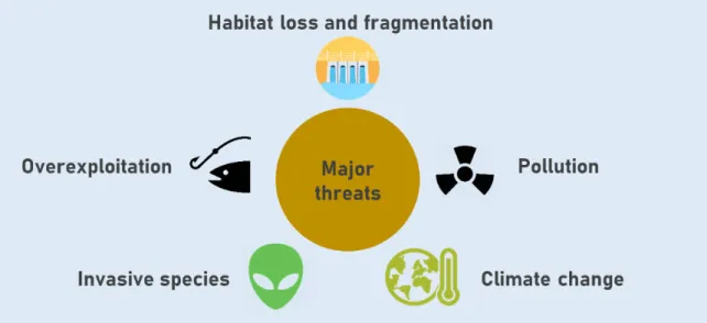
Figure 1 – Diagram with the five major threats to freshwater biodiversity.
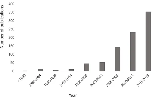
Figure 2 – Number of publications until September 2019 (N=800) retrieved from SCOPUS database using the words ‘freshwater protected areas’.
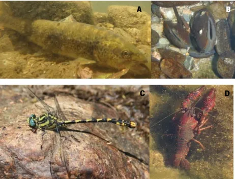
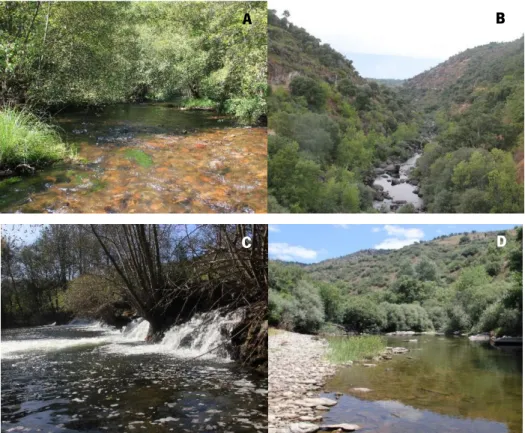
Figure 3 – Examples of faunal diversity found in Montesinho Natural Park and surrounding areas: brown trout Salmo trutta (A); pearl mussel Margaritifera margaritifera (B); dragonfly Macromia splendens (C); Louisiana red swamp crayfish Procambarus clarkii (D). Courtesy of Ronaldo Sousa. Figure 4 – Rivers surveyed in this study: Mente (A), Rabaçal (B), Tuela (C) and Sabor (D). Courtesy of Ronaldo Sousa.
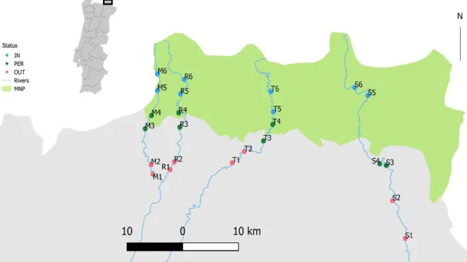
Figure 5 – Map of the surveyed area showing the location of the 24 sampling sites in Mente (M), Rabaçal (R), Tuela (T) and Sabor (S) Rivers.
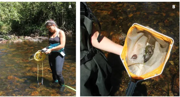
Figure 6 – Measurement of abiotic variables with a multi-parameter probe (A) and hand net used to collect the macroinvertebrates (B). Courtesy of Ronaldo Sousa.
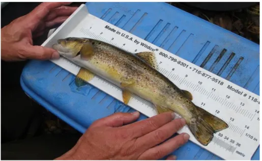
Figure 7 – Divers surveying freshwater mussels by snorkelling. Figure 8 – Measurement of a brown trout Salmo trutta in the field.
Figure 9 – Principal Components Analysis (PCA) showing the arrangement of the 24 sampling sites based on the abiotic factors measured. PC1 explains 38.1% of all variance and PC2 21.8%. Figure 10 - Multidimensional scaling (MDS) of the macroinvertebrate communities showing sampling sites and park status.
Figure 11 – Richness (A), Abundance (B), Shannon-Wiener diversity (C) and Pielou’s evenness (D) of the macroinvertebrate communities outside (pink), periphery (green) and inside (blue) the park. White circles represent the average values. Boxplots show median values (central line), the range from the 25th to 75th percentile (box) and the largest and lowest value within 1.5 times interquartile range below and above the 25th and 75th percentile (whiskers) and dots represent extreme values.
Figure 12 –IBMWP (A), IASPT (B) and %EPT (C) water quality indices outside (pink), periphery (green) and inside (blue) the park. White circles represent the average values. Boxplots show median values (central line), the range from the 25th to 75th percentile (box) and the largest and
ix
lowest value within 1.5 times interquartile range below and above the 25th and 75th percentile (whiskers) and dots represent extreme values.
Figure 13 – Abundance (ind. CPUE) of pearl mussel Margaritifera margaritifera outside (pink), periphery (green) and inside (blue) the park. White circles represent the average values. Boxplots show median values (central line), the range from the 25th to 75th percentile (box) and the largest and lowest value within 1.5 times interquartile range below and above the 25th and 75th percentile (whiskers) and dots represent extreme values.
Figure 14 – Abundance (ind.CPUE) of the pearl mussel Margaritifera margaritifera on Mente (A), Rabaçal (B) and Tuela (C) Rivers in each site outside (pink), in the periphery (green) and inside (blue) the park. White circles represent the average values. Boxplots show median values (central line), the range from the 25th to 75th percentile (box) and the largest and lowest value within 1.5 times interquartile range below and above the 25th and 75th percentile (whiskers) and dots represent extreme values. Different letters indicate significant differences among status.
Figure 15 - Length (mm) of the pearl mussel Margaritifera margaritifera outside (pink), periphery (green) and inside (blue) the park. White circles represent the average values. Boxplots show median values (central line), the range from the 25th to 75th percentile (box) and the largest and lowest value within 1.5 times interquartile range below and above the 25th and 75th percentile (whiskers) and dots represent extreme values. Different letters indicate significant differences among status.
Figure 16 - Length (mm) of Margaritifera margaritifera in Rabaçal (A) and Tuela (B) Rivers in each site outside (pink), in the periphery (green) and inside (blue) the park. White circles represent the average values. Boxplots show median values (central line), the range from the 25th to 75th percentile (box) and the largest and lowest value within 1.5 times interquartile range below and above the 25th and 75th percentile (whiskers) and dots represent extreme values. Different letters indicate significant differences among status.
Figure 17 - Multidimensional scaling (MDS) of the fish communities showing sampling sites and park status.
Figure 18 - Richness (A), Abundance (B), Shannon-Wiener diversity (C) and Pielou’s evenness (D) of the fish communities outside (pink), periphery (green) and inside (blue) the park. White circles represent the average values. Boxplots show median values (central line), the range from the 25th to 75th percentile (box) and the largest and lowest value within 1.5 times interquartile range below
x
and above the 25th and 75th percentile (whiskers) and dots represent extreme values. Different letters indicate significant differences among status.
Figure 19 – Abundance (ind.CPUE) of Salmo trutta (A), Squalius alburnoides (B), Luciobarbus bocagei (C), Squalius carolitertii (D), Pseudochondrostoma duriense (E), Cobitis calderoni (F) and Cobitis paludica (G) outside (pink), in the periphery (green) and inside (blue) the park. White circles represent the average values. Boxplots show median values (central line), the range from the 25th to 75th percentile (box) and the largest and lowest value within 1.5 times interquartile range below and above the 25th and 75th percentile (whiskers) and dots represent extreme values. Different letters indicate significant differences among status.
Figure 20 – Length (cm) of Salmo trutta (A), Squalius alburnoides (B), Luciobarbus bocagei (C), Squalius carolitertii (D), Pseudochondrostoma duriense (E), Cobitis calderoni (F) and Cobitis paludica (G) outside (pink), in the periphery (green) and inside (blue) the park. White circles represent the average values. Boxplots show median values (central line), the range from the 25th to 75th percentile (box) and the largest and lowest value within 1.5 times interquartile range below and above the 25th and 75th percentile (whiskers) and dots represent extreme values. Different letters indicate significant differences among status.
Figure 21 – Before (2012) (A) and after (2017) (B, C) the construction of a weir with the goal of creating an artificial beach for visitors inside Montesinho Natural Park. Courtesy of Ronaldo Sousa. Figure 22 – Macroinvertebrates and fish richness outside (pink), in the periphery (green) and inside (blue) the park. The size of the circles is proportional to the value of richness.
Figure 23 – Species of conservation importance (Vulnerable, Endangered or Critically Endangered) in each site for all the rivers studied, outside (pink), in the periphery (green) and inside (blue) the park. The size of the circles is proportional to the number of species.
xi
List of Tables
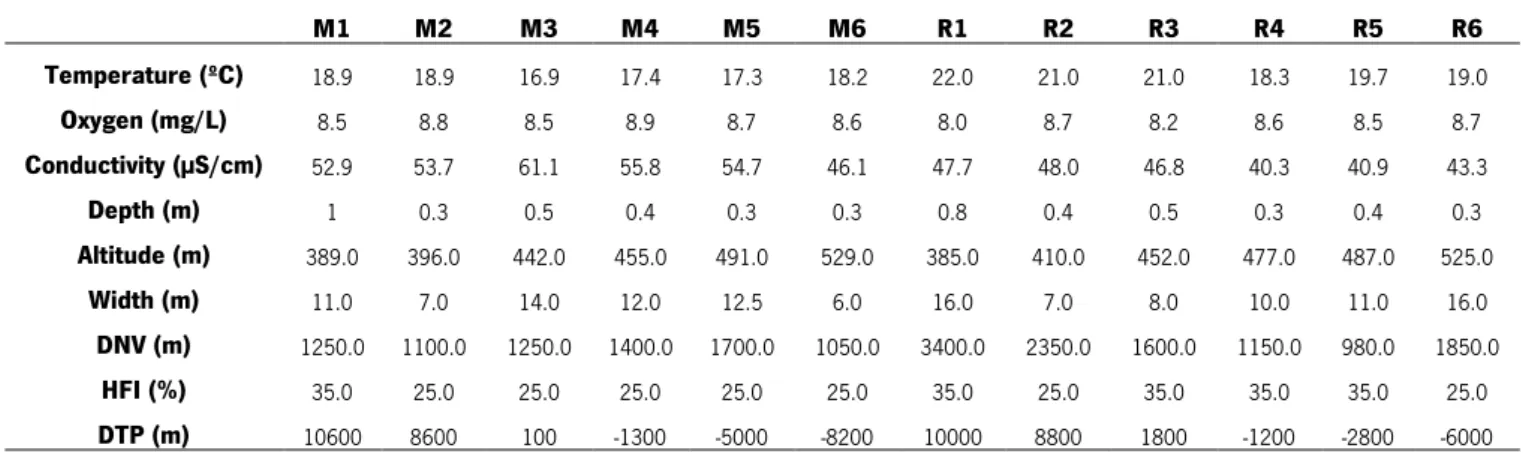
Table 1 – Abiotic characterization in all sampling sites in the Mente, Rabaçal, Tuela and Sabor Rivers.
Table 2 – Water quality index for all the sampling sites in Mente, Rabaçal, Tuela and Sabor Rivers. IBMWP quality scores: >100 – very good; 100-61 – good; 36-60 – polluted; 16-35 – very polluted; <16 – extremely polluted (after Alba-Tercedor and Sánchez-Ortega, 1988).
Table S1 - Results of the Principal Components Analysis based on the abiotic data. Table S2 – Contribution of the abiotic variables to each of the first three PCA axis.
Table S3 – Abundance of macroinvertebrates taxa in Mente, Rabaçal, Tuela and Sabor Rivers. Table S4 – SIMPER analysis results showing the macroinvertebrate taxa contributing the most to the average dissimilarity between status (outside, in the periphery and inside the park).
Table S5 – Results of the linear regressions between abiotic factors and macroinvertebrates richness (S), abundance (N), Shannon-Wiener diversity (H’), Pielou’s evenness (J’), and IBMWP, IASPT and %EPT water quality indices. ns – non significant; * - statistically significant.
Table S6 – Abundance (ind.CPUE) of Margaritifera margaritifera in Mente, Rabaçal and Tuela Rivers.
Table S7 –Fish species abundance (ind.CPUE) in Mente, Rabaçal, Tuela and Sabor Rivers. Table S8 – Results of the PERMANOVA analysis on fish communities along park status (outside, in the periphery and inside the park) and overall results of the pairwise tests.
Table S9 - SIMPER analysis results showing the fish species contributing the most to the average dissimilarity between status (outside, in the periphery and inside the park).
Table S10 – Results of the linear regressions between abiotic factors and fish richness (S), abundance (N), Shannon-Wiener diversity (H’) and Pielou’s evenness (J’). ns – non significant; * - statistically significant.
1
1.
Introduction
1.1
Importance of freshwater ecosystems
Freshwater ecosystems are essential to environmental health, economic wealth and human well-being (Grill et al., 2019). The integrity of freshwater ecosystems is of vital importance, as the fresh water supply stands in the top ten (listed as fourth) of the most pressing concerns for human survival (WEF, 2019). Humans use freshwater ecosystems for drinking and irrigation purposes, waste disposal, transportation, energy production, fisheries, and for harvesting plants and minerals (Strayer and Dudgeon, 2010). All these services provided by freshwater ecosystems have high economic value.
Covering approximately 1% of Earth’s surface, lakes and rivers host 9.5% of all animal species (Dudgeon et al., 2006; He et al., in press) turning freshwater ecosystems areas of high biodiversity. Still, this biodiversity faces numerous threats responsible for large declines in abundance and spatial distribution of many species. For example, 44% of freshwater mussels, 37% of fish, 23% of amphibians, 19% of reptiles, 15% of mammals and dragonflies, 13% of birds, 9% of butterflies and 7% of aquatic plants are threatened in Europe (Freyhof and Brooks, 2011). According with the 2018 World Wide Fund for Nature and its Living Planet Index, freshwater vertebrates (one-third of all vertebrates) declined in their abundance and spatial distribution by 83% compared to 1970 data. This is particularly alarming if compared to the declines reported for marine and terrestrial ecosystems with values around 36% and 38%, respectively (He et al., in press; Reid et al., 2019). Several freshwater species suffered pronounced range contractions, like the European sturgeon (Acipenser sturio) that was extirpated from all major European rivers, and is now confined to the Garrone River in France. Other species such as the baiji (Lipotes vexillifer) and the Chinese paddlefish (Psephurus gladius) are considered extinct due to human activities and intrinsic factors (e.g. long life cycle and lower fecundity) of their biology (He et al., in press). Besides human activities, many freshwater species are restricted to small isolated areas and this situation is responsible for high rates of endemism and increased risk of extinction (Abell et al., 2008; Dudgeon et al., 2006). Given the remarkable biodiversity, the vulnerability and the level of endemism present in freshwater ecosystems these areas should, in theory, be considered a conservation priority. Unfortunately that is not the case since, for example, conservation literature tends to be biased towards terrestrial systems with 81% of research articles focused on these ecosystems (Di Marco et al., 2017).
2
Under the current biodiversity crisis, species are declining at an alarming rate (Olson et al., 2001) primarily due to human activities and global consumption of natural resources (Garcia-Moreno et al., 2014). This has led to chemical, physical and biological alterations in all ecosystems, being freshwater ecosystems no exception (Carpenter et al., 2011). Human well-being is the priority when it comes to decision making and policy, resulting in loss of biodiversity that supports some of these same priorities (Cowx and Portocarrero-Aya, 2011; Darwall et al., 2018). The biggest threats to freshwater ecosystems are related to overexploitation, climate change, introduction of non-native species, pollution, changes in water flow and destruction and fragmentation of habitats (Figure 1) (Carpenter et al., 2011; Dudgeon et al., 2006). Overexploitation is mostly affecting fishes (overfishing), amphibians and reptiles (Naylor et al., 2000), but even macroinvertebrates can be highly explored (see for example some freshwater bivalves in Lopes-Lima et al., 2017 and Zieritz et al., 2018). The increasing water temperature related with the higher global atmospheric temperature causes the depletion of dissolved oxygen in water, affects the physiology, phenology and distribution of many species (Carpenter et al., 2011; Mohseni et al., 2003) and can even cause direct mortality (Nogueira et al., in press). Freshwater ecosystems are also heavily impacted by the introduction of non-native species (Sala et al., 2000; Strayer, 2010), affecting ecosystems structure and functioning as well as their biotic and abiotic interactions (Sousa et al., 2009; Sousa et al., 2019). Even though some species have been introduced accidentally, many have been deliberately introduced by humans to serve their needs (e.g. aquaculture, sport fishing and pest control) (Carpenter et al., 2011; Sousa et al., 2014). Changes in the land use of riparian areas and watersheds (mostly due to agricultural expansion) alters de input of water, sediments, nutrients and other chemicals leading to eutrophication and pollution that affects natural communities, alters biogeochemical cycles and disturbs the habitat for many species (Dudgeon et al., 2006; Quinton et al., 2010; Strayer and Dudgeon, 2010). As fresh water is not evenly available in time and space, there is a need to control water reserves (mostly to agriculture, industry and domestic use) through the construction of dams and levees. These physical obstacles alter the connectivity of rivers, capture about 25% of global sediment load (Vörösmarty and Sahagian, 2000), can heavily change the natural river flow, impair fish (and other species) migration and exacerbate the occurrence of infectious diseases caused by standing-water related parasites (Carpenter et al., 2011). Globally, there is close to 2.8 million dams (reservoir area >1000 m2) fragmenting rivers and altering their courses and this number will rise in the next years in areas such as Amazon, Mekong, Congo and the Balkans basins (Grill et al., 2019). All these threats may operate synergistically, as flow
3
modification can be exacerbated by climate change (more frequent floods and droughts) (Vörösmarty et al., 2010), or non-native species that are more likely to proliferate in human modified environments (Gaertner et al., 2017). Besides these persistent threats, new emerging ones have been identified affecting freshwater biodiversity and are related to e-commerce, algal blooms, engineered nanomaterials, microplastic pollution, urban light and noise, increase salinization and decrease of calcium (described in Reid et al., 2019).
Figure 1 – Diagram with the five major threats to freshwater biodiversity.
1.2 Freshwater Protected Areas
A variety of measures are available to manage freshwater ecosystems and address biodiversity decline, from small-scale river restoration to a large-scale implementation of protected areas (PAs) (Gray et al., 2016; Pimm et al., 2018). According to IUCN’s standard designation a PA is ‘an area of land/or sea especially dedicated to the protection and maintenance of biological diversity, and of natural and associated cultural resources, managed through legal or other effective means’. The philosophy beyond the rationale to implement a PA has evolved throughout the years, with shifting views about the best way of protecting nature. It went from the protection of areas with high nature scenic value (1960-70’s), to nature apart from humans (1980-90’s), to the importance of ecosystem services (2000-05’s) and finally to the most recent dynamic relation between nature and people (Mace, 2014). These views were responsible for the evolution of the PA concept from
4
the protection of terrestrial biodiversity islands surrounded by human disturbed areas to the current emphasis on the importance of socioecological systems (Palomo et al., 2014).
Since we cannot protect all regions with some biological importance, the selection of priority areas is fundamental. This can be made using species data through two main methodologies: one is based on scoring the sites according to criteria of species vulnerability, rareness and richness (Margules and Usher, 1981); the other, more recent, is based on systematic conservation planning (Margules and Pressey, 2000). Systematic conservation planning aims to represent a maximum of species in a priority area, in the most cost-effective way, which is done by identifying the conservation goals (e.g. target species and area) and available resources (e.g. socioeconomic cost). Systematic conservation planning uses the concept of complementarity, which is defined as the gain in representativeness in biodiversity when a site is added to an area (Hermoso et al., 2016). Ideally, a PA should be designed with the intent of protecting all faunal groups, but due to limited biological data and resources, some species (usually defined as surrogate species) are used as proxy to the presence of others (Caro, 2010). However, this approach can be misleading and can disregard rare and spatially restricted species, as demonstrated by Stewart et al., (2018) when these authors found limited congruence of priority watersheds for 72 species of freshwater fish, amphibians, reptiles and mussels. The effectiveness of a PA can be measured by its representativeness and persistence, meaning that reserves must include a full range of biodiversity items (e.g. genetic, taxonomic and ecosystems) and that this biodiversity has the capacity to survive, maintain natural processes and populations, as well as withstand threats (Margules and Pressey, 2000).
Given the potential role of PAs in preserving biodiversity, freshwater ecosystems have been also a target of worldwide conservation efforts. Examples include the USA’s National Wild and Scenic Rivers, developed for protecting freshwater systems (209 rivers designated, including the Mississippi River) due to their aesthetic value; United Kingdom’s Special Areas of Conservation, developed to protect rare and vulnerable species such as the Borgie River in Scotland or the Avon River in England, that use surrogate species like the pearl mussel Margaritifera margaritifera, plants such as Ranunculus sp. or fish such as the Atlantic salmon Salmo salar; or the Canadian Heritage Rivers System that include, among others, the longest protected river, Fraser River, with 1375 km. There are also examples of Ramsar Sites designated with the goal of protecting wetlands, such as the Lake Baikal in Russia, or the Danube Delta in Romania (Saunders et al., 2002). More recently, the concept of Key Biodiversity Areas (KBAs) developed by IUCN, uses a standard criterion to
5
identify freshwater regions capable of maintaining endangered species (but see Butchart et al., 2015).
Despite this increasing interest in conserving freshwater ecosystems there is still a high discrepancy between the protected area coverage in terrestrial, marine and freshwater systems, with 57%, 37% and 6%, respectively (Di Marco et al., 2017). Currently, 15.4% of terrestrial land surface is covered by PAs, and CBD’s Aichi Biodiversity Target 11 has the goal to protect at least 17% (including inland waters) by 2020 (CBD; Convention on Biological Diversity 2010; Pimm et al., 2018). This expansion should be planned towards a more balanced distribution in terrestrial, marine and freshwater ecosystems. Since the CBD report joined both terrestrial and aquatic systems it is difficult to differentiate between them, and assess the increased coverage for each one. Abell et al. (2011) proposed a method that prioritizes possible PAs by overlapping areas that host rare and endemic species from both the terrestrial and freshwater domains. This pragmatic approach is of major importance since funds for conservation are scarce and besides being frequent in marine and terrestrial planning, freshwater systems are lacking in spatial prioritisation (Abell et al., 2007; Juffe-Bignoli et al., 2016). For example, in Europe, Natura 2000 represents the most important conservation network and PAs are based on Birds and Habitats Directives (Natura 2000: http://ec.europa.eu). Although their primary goal is to protect biodiversity, the efficiency in protecting freshwater habitats and species has been questioned (Hermoso et al., 2015), as we cannot simply expect that they will be accidentally included in terrestrial PAs (Abell et al., 2011). For example, Carrizo et al. (2017) showed a great mismatch between the existing PAs and areas of critical importance to freshwater biodiversity, with 84% of threatened freshwater megafauna falling outside the reserves, proving the lack of representativeness of aquatic biodiversity when planning a PA.
Despite that legal protection may enhance the diversity and abundance of some species there are several examples of decline and loss of freshwater biodiversity inside PAs. Examples include the disappearance of amphibians due to the chytrid fungus infection (Skerratt et al., 2007) or the extirpation of native fish and mollusks due to the stocking of non-native fish in Banff National Park in Canada (Schindler, 2000). In addition, the implementation of management measures is much more developed in terrestrial and marine counterparts (Collier, 2011), turning more difficult the implementation of a PA in a freshwater ecosystem (Hermoso et al., 2016). These difficulties to conserve freshwater biodiversity are generally exacerbated by the intricate complexity of river connections, the high spatial and temporal variability, the lack of control of external processes and
6
threats (Roux et al., 2008; Collier, 2011) and patchy information on freshwater species (Abell et al., 2011). For example, IUCN Red List assessment lacks information on many freshwater species, and the knowledge of fish migration routes and spawning grounds is also limited (He et al., in press). If some of this basic information is lacking for a faunal group such as migratory fish, we may think that the level of ignorance for basic biological features in macroinvertebrates is even higher. In addition, and although rivers are often chosen as ecologic corridors, many times these same rivers inside PAs are used as simple administrative boundaries (Hermoso et al., 2015). For example, in Portugal the Peneda Gerês National Park and International Tejo Natural Park are two important PAs and the Cávado and Tejo Rivers function in several kilometres as the border of the two parks, respectively. Finally, the hydrological connectivity in a river (longitudinal, lateral and vertical) also poses a great challenge for the design and management of PAs, and so, traditional ideas used in terrestrial ecosystems are not adequate for freshwater protection (Abell et al., 2007). Longitudinal connectivity is crucial to maintain ecological processes such as species migration, their reproduction, long-term population dynamics and gene flow; lateral connectivity allows the exchange of matter and energy between rivers and floodplains or other habitats (e.g. lakes); and vertical connectivity links the surface and groundwater systems (Hermoso et al., 2011). Spatial-temporal connectivity also maintains important ecological processes like the periodic migrations or the dispersal to refuge areas (Hermoso et al., 2016). All these details turn the implementation of an effective freshwater PA much more difficult when compared to terrestrial or marine PAs. Ideally, and for a freshwater PA be really effective, it should cover the whole watershed (Abell et al., 2017; Rodriguez-Olarte et al., 2011) and take in account that possible disruptive factors (pollution, flow alteration and introduction of non-native species) propagate along the rivers (Hermoso et al., 2015). Mitigation of point source pollution, the management of fisheries and non-native invasive species, the restriction of human activities and land use around the watershed (e.g. riparian vegetation and floodplain), as well as restoration of the normal water flow and connectivity are essential to achieve a proper protection of aquatic biodiversity (Abell et al., 2011; Dudgeon et al., 2006; Nel et al., 2007; Saunders et al., 2002). However, the reality is that many of the world’s rivers are barely protected in their upland areas, being that only 11% of rivers (by length) benefit from integrated management (Abell et al., 2017). Therefore, and as a more realistic management tool, sub-catchments (contributing catchment around a river segment) are often considered spatial planning units in freshwater conservation (Reis et al., 2019).
7
Designing a freshwater PA has also socioeconomic and political constrains. Areas with/around water bodies are frequently disputed for industrial (e.g. construction of dams), commercial (e.g. extraction of natural resources) or housing purposes, and so new reserves are often chosen in remote or low productivity areas for convenience. This situation usually does not contribute for a well representation of their biodiversity. Anyway, a few studies have already started to use a systematic conservation planning approach for freshwater ecosystems (e.g. Abell et al., 2007; Lawrence et al., 2011) and, for example, Hermoso et al. (2011) used a well-known conservation planning software package – MARXAN – to penalize management measures that do not include upstream catchments.
Finally, and as the interest about ecosystems services is growing, freshwater conservation could enhance several important functions and services such as water supply, nutrient cycling and water regulation (Palomo et al., 2014). Thus, a framework for freshwater conservation planning is urgently needed, and an increase in the exchange of information between science, policy and management would strongly benefit freshwater ecosystems (Darwall et al., 2018).
1.3 Statement of the problem and main objectives
Previous studies have shown that some PAs have a positive influence on freshwater biodiversity. For example, fish population structure tends to improve (i.e. higher fish length and biomass) inside protected areas where fishing is regulated/prohibited (Baird and Flaherty, 2005; Cucherousset et al., 2007; Keppler et al., 2017; Sanyanga et al., 1995). On the other hand, other studies showed no differences in biodiversity patterns for macroinvertebrates and fish outside and inside PAs (Heino et al., 2009; Srinoparatwatana and Hyndes, 2011) or even a negative effect on freshwater turtles inside Brazilian PAs (Fagundes et al., 2016). To the best of our knowledge there is no such an assessment in Portugal, and very few worldwide. In fact, and although 800 studies were retrieved in our search in the SCOPUS database using the words ‘freshwater protected areas’ (Figure 2), the reality is that very few of these studies really assess the effectiveness of protected areas in freshwater ecosystems.
8
Figure 2 – Number of publications until September 2019 (N=800) retrieved from SCOPUS database using the words ‘freshwater protected areas’.
There are several doubts concerning the use of terrestrial biodiversity as a surrogate to freshwater biodiversity. So, theoretically, land based approaches only benefit freshwater species to a certain extent, if at all. Given this uncertainty about the possible positive (neutral or even negative) influence of terrestrial PAs, this study aims to assess if the Montesinho Natural Park (MNP), NE of Portugal, affects the freshwater biodiversity. For this, two faunal groups (macroinvertebrates and fishes), as well as abiotic data, were sampled inside, outside and in the periphery of the MNP. The macroinvertebrate communities are very diverse and abundant, play an important ecological role in freshwater ecosystems as a link of energy between different trophic levels and are important in processes such as nutrient cycling and decomposition (Covich et al., 1999). In addition, macroinvertebrates are used to calculate several water quality indices (e.g. IBMWP, IASPT and %EPT). Among the macroinvertebrates sampled a special attention was given to bivalves, mainly the freshwater pearl mussel M. margaritifera, due to their conservation status (i.e. listed as Critically Endangered in Europe) (Geist, 2010). Fish communities were also sampled and studied because of their ecological role (some species have high abundance and trophic importance) and due to their conservation, social and cultural relevance (Closs et al., 2015).
Information collected was used to calculate water quality and diversity indices and comparisons between the three park status (i.e. inside, periphery and outside) were performed. If the terrestrial biodiversity can be considered a surrogate for freshwater biodiversity it would be expected that improved abiotic and biological conditions will be found inside the park. In addition, our results can
0 50 100 150 200 250 300 350 400 N um ber of p ubli cat ion s Year
9
function as a reference of the abiotic and biological conditions of the study area. This information can be used for future comparisons and help politicians, managers and stakeholders to make better decisions (e.g. define areas that are not currently included in the park but could be in the future) concerning the conservation of the freshwater biodiversity present in the MNP and surrounding areas.
10
2.
Material and methods
2.1 Study area
Montesinho Natural Park was created in 1979 and is located in northeast Portugal (Trás-os-Montes region), which includes Vinhais and Bragança counties. The park is located from 41º 43’47’’ to 41º 59’ 24’’ N and 6º 30’ 53’’ to 7º 12’ 9’’ W, and is a category V in the IUCN assessment. By definition a Category V protected area is ‘where the interaction of people and nature over time has produced an area of distinct character with significant ecological, biological, cultural and scenic value: and where safeguarding the integrity of this interaction is vital to protecting and sustaining the area and its associated nature conservation and other values’. MNP was designed with the focus on birds, terrestrial vertebrates and plants. There is a significant biodiversity, however much lower than in the past, having suffered a tremendous lost in the amount of native forest, a drastic reduction of wolf abundance, and the disappearance of bear and lynx (ICNF, 2019).
Climate is Mediterranean with influence from the Atlantic Ocean (Oliveira et al., 2012), where the medium annual temperatures vary between 8.5 and 12.8ºC. Annual average precipitation is 1000-1600 mm, with highest values in winter and an almost absence of precipitation in the summer. Floods may occur in winter/early spring and droughts in summer/early autumn (Sousa et al., 2015).
The geology of the park and surrounding area is very complex, dominated by schist, granite, amphibolite and migmatite, and also the occurrence of basic and ultrabasic rock formations (e.g. peridotites and serpentines). Its geomorphology is characterized by the existence of mountains and plateaux cut by deep river valleys, where altitude range between 438 and 1481 m, being the highest values registered in Montesinho and Coroa mountains.
The vegetation of the study area is very diverse, mostly influenced by its geographic location/climate and complex geology, and include species such as the oak Quercus pyrenaica, the chestnut Castanea sativa and the holm oak Quercus rotundifolia. The scrubland is composed of heather Erica australis and Erica umbellate, the rockrose Cistus ladanifer or Genista tridentataand meadows with ryegrass Lolium rigidum, among many other species. Riparian vegetation includes the alder Alnus glutinosa, the ash Fraxinus sp. and the willow Salix sp. Species of conservation value include matgrass Nardus stricta, the crossleaf heath Erica tetralix and the needle furze Genista anglica.
11
A significant presence of birds is noted in MNP, constituting a nesting place for 125 of the 150 species described in this protected area. Rare species like the eagle Aquila chrysaetos, the black stork Ciconia nigra or the red-backed shrike Lanius collurio can be found. Terrestrial mammals like the wild boar Sus scorfa, the Iberian wolf Canis lupus signatus, the deer Cervus elaphus and roe deer Capreolus capreolus can also be found, as well as aquatic mammals like the water desman Galemys pyrenaicus and the otter Lutra lutra. The rivers that cross the park are important habitats for the brown trout Salmo trutta (Figure 3A) and Iberian endemic cyprinids such as Pseudochondrostoma duriense, Achondrostoma arcasii, Squalius carolitertii, Squalius alburnoides and Luciobarbus bocagei.
Some species with conservation importance also find a refuge in the MNP and surrounding areas, including Iberian endemic species such as the water lizard Lacerta schreiberi or the frog Rana iberica. Species listed under IUCN Red List of Threatened Species like the pearl mussel Margaritifera margaritifera (Endangered) (Figure 3B), Potomida littoralis (Endangered), the Iberian loach Cobitis calderoni (Endangered) or the dragonfly Macromia splendens (Vulnerable) (Figure 3C) are also present in the MNP and surrounding areas.
The presence of non-native invasive species is well noted in the study area, with examples including the crayfishes Procambarus clarkii (Figure 3D) and Pacifastacus leniusculus, the American mink Neovison vison or the tree of heaven Ailanthus altissima.
Figure 3 – Examples of faunal diversity found in Montesinho Natural Park and surrounding areas: brown trout Salmo trutta (A); pearl mussel Margaritifera margaritifera (B); dragonfly Macromia splendens (C); Louisiana red swamp crayfish Procambarus clarkii (D). Courtesy of Ronaldo Sousa.
A B
12
The human pressure within the MNP is low, with a total area of 75 000 hectares and a population under 9000 inhabitants throughout 88 villages that tends to decline due to the ageing population and the abandonment of rural areas. Human occupation is mostly related to subsistence agriculture, associated with the cultivation of potatoes, chestnut, rye and permanent grassland. Rivers surveyed in this study are included in the Tua: Mente (Fig. 4A), Rabaçal (Fig. 4B) and Tuela (Fig. 4C) Rivers and Sabor basins: Sabor River (Fig. 4D). Mente is a tributary of Rabaçal, which in turn is connected to Tuela to form the Tua River just upstream of the city of Mirandela. All the four rivers are born in Spain with extensions of 120 km, 57 km, 88 km and 102 km respectively (Oliveira et al., 2012). All rivers belong to the Douro basin, being Sabor and Tua Rivers (in addition to Tâmega River) the most important tributaries in the right side of the basin in Portuguese territory. Areas around the four rivers have very low human pressure, being all rivers quite undisturbed (Sousa et al., 2012, 2015, 2018). In the study area, Rabaçal (Rebordelo and Sonim) and Tuela (Nunes and Trutas) Rivers have two small small hydropower plants each and the Sabor River (Gimonde) just one.
Figure 4 – Rivers surveyed in this study: Mente (A), Rabaçal (B), Tuela (C) and Sabor (D). Courtesy of Ronaldo Sousa.
A B
13
2.2 Sampling strategies
Field surveys were carried out between middle July/early August 2018, in a total of 24 sampling sites: 6 sites for each of the four rivers surveyed: Mente (M1, M2, M3, M4, M5 and M6), Rabaçal (R1, R2, R3, R4, R5 and R6), Tuela (T1, T2, T3, T4, T5, and T6) and Sabor (S1, S2, S3, S4, S5 and S6) Rivers (Figure 5). Sites referred with the numbers 1 and 2 correspond to areas outside of the MNP, 3 and 4 to areas in the periphery of the MNP, and 5 and 6 correspond to areas inside the MNP. Therefore, along the entire study, sites location is referred as status, each one characterized by a colour: pink (outside the park), green (periphery of the park) and blue (inside the park). Each site was georeferenced and photographed. Map of the surveyed area was developed in QGIS 2.18.26 using the coordinates of each site and Bing Aerial web mapping service.
Figure 5 – Map of the surveyed area showing the location of the 24 sampling sites in Mente (M), Rabaçal (R), Tuela (T) and Sabor (S) Rivers.
For the abiotic characterization, water temperature, conductivity and dissolved oxygen were analysed in situ in all sites with an HACH HQ 40d multi-parameter probe (Figure 6A). Channel width and middle channel depth were measured with a tape.
Macroinvertebrates were sampled following the Water Directive Framework (INAG, 2008). This was made using a hand net with a mesh of 0.05 cm and a width of 25 cm (Figure 6B). Each site corresponds to a river stretch with a total length of 50 m and the sampling covered all type of
14
habitats (e.g. lentic and lotic, banks and centre of the channel) and sediments (e.g. pebbles, cobbles, sand, silt, clay, macrophytes). In each site, 6 replicates were performed with 1 m long and 0.25 m wide. The sampling net was placed counter-current while the substratum was moved, pushing the macroinvertebrates into the net. Organisms were stored in the field in labelled flasks containing alcohol (70%) to be later sorted and identified to the family level. Classification of all organisms was performed with a binocular lens, using Tachet et al., (2003) identification keys.
Figure 6 – Measurement of abiotic variables with a multi-parameter probe (A) and hand net used to collect the macroinvertebrates (B). Courtesy of Ronaldo Sousa.
Regarding the possible presence of freshwater mussels (Order Unionida), river stretches of 50 m containing different habitats (riffles, pools, near the banks and in the centre of the channel), as described for macroinvertebrates (see above), were surveyed. Individuals were surveyed by snorkelling and hand searching. Four to six dives with a duration of five minutes each were performed by two experienced divers in each site (Figure 7). The number of replicates was higher in sites that had lower abundances. All the live specimens were counted and measured with a Vernier calliper (to 0.1 mm), and posteriorly returned to their habitat in their original position. Abundance is expressed as the number of individuals for each five minutes – individuals per catch per unit effort (ind.CPUE), following the methodology described in Sousa et al. (2018, 2019). The interpretation of results takes in consideration the possible bias from smaller mussels or buried ones that escaped researcher’s sight, although it should be minimal since the surveys were always performed by the same divers in similar visibility conditions.
15
Figure 7 – Divers surveying freshwater mussels by snorkelling.
Fish fauna was surveyed by electrofishing following the guidelines described in the Water Directive Framework (INAG, 2008). All sites selected were representative of the river, containing all type of habitats (excluding deeper areas) with a minimum length of 100 m. Two experienced researchers performed the fisheries using a portable equipment Hans Grassl with a pulsed DC-300-600 V generator. The fisheries were timed, ranging from 20-40 minutes. The stunned fish were collected in water recipients and posteriorly identified to the species level, counted and measured with a ruler (Figure 8). All specimens were released after the collection of these data. Fish abundance was expressed as the number of individuals in a 20-minute fishery – individuals per catch per unit effort (ind.CPUE).
16
2.3 Data analysis
Abiotic characterization consisted on the analysis of nine variables including water temperature, conductivity, dissolved oxygen and river width and depth (as described above) plus altitude, distance to the nearest village (DNV), distance to the limits of the park (DTP) and Human Footprint Index (HFI). Altitude and DNV were calculated using Google Earth, being that DNV was considered to be the minimum distance in a straight line from the sampling site to the nearest village. The DTP was calculated using QGIS (2.18.26) measuring tool, being the distance from sampling sites to the nearest limit of MNP, in which positive values relate to sites outside the park, and negative ones to sites inside the park. As for the HFI, it measures the human pressure compiling information of population density, human land use and infrastructure (e.g. built-up areas, crop land, pasture and night-time lights) and human access (e.g. roads, railroads, and navigable waterways). HFI is expressed as percentage and is available at ArcGIS (https:// arcgis.com). In the particular case of this study, we used the average percentage value described for each sampling site. All abiotic data was normalised and used to perform a Principal Component Analysis (PCA). This multivariate analysis allowed to sort the different sites according to the variables in study and was performed on Primer 6 (version 1.0.3, Primer-E Ltd, Plymouth).
The macroinvertebrate communities were analysed with a Multidimensional scaling (MDS), in which the data was previously log transformed and used to make a similarity matrix using the Bray-Curtis distance. To evaluate the influence of the park status on the macroinvertebrate communities in the 24 sites, a one-way PERMANOVA was designed with status (3 factors: outside, periphery and inside) as a fixed factor. The test considered 9999 permutations, but when the number was lower than 150 the Monte Carlo test p-value was considered. A similarity percentage (SIMPER) analysis was performed (cut-off 90%) to assess the taxa contributing to the dissimilarity between the tree different park status. Richness (number of families; S), abundance (N), and diversity indices Shannon-Wiener (H’) and Pielou’s evenness (J’) were calculated using DIVERSE function. All the analyses mentioned above were computed on Primer 6 (version 1.0.3, Primer-E Ltd, Plymouth). Also, regression analyses were performed with dependent variables: S, N, H’, J’, IBMWP, IASPT and %EPT against independent predictor variables: temperature, oxygen, conductivity, depth, altitude, width, HFI, DNV and DTP using Minitab 14. Water quality indices were also determined, including the IBMWP (Iberian Biological Monitoring Working Party) (Alba-Tercedor and Sánchez-Ortega, 1988), the IASPT (Iberian Average Score Per Taxa) (Alba-Tercedor, 2000) and the %EPT (percentage of Ephemeroptera, Plecoptera and Tricoptera families). A one-way ANOVA was
17
performed to test possible differences in richness, abundance, H’ index, J’ index, IBMWP, IASPT and %EPT between the different park status.
Abundance and length of the pearl mussel M. margaritifera were analysed compiling all three rivers in which the species is present (Mente, Rabaçal and Tuela Rivers) and also each river individually for a more detailed assessment. A one-way ANOVA was carried out in order to assess possible differences in abundance and length between park status. A Tukey test was performed with length data to detect where the differences exist. Regarding the analyses on each river, a one-way ANOVA was performed to compare pearl mussel’s abundance in the different park status for the Rabaçal and Tuela Rivers. For this, data was previously transformed (square root) to achieve homoscedasticity. A multiple comparison test (Tukey) was conducted in the Tuela River. In Mente River, pearl mussels were only found outside the park (see results section) and so no further statistical analysis was performed. A one-way ANOVA was also performed to check possible differences in pearl mussel’s length between park status for Rabaçal and Tuela Rivers, as well as a Tukey test. All these statistical analyses were performed with R Studio (version 1.1.463). Finally, a linear regression tested a possible relation between pearl mussel abundance and its fish host (i.e Salmo trutta) abundance on Minitab 14.
Fish communities were analysed with a MDS, in which the data was previously log transformed and used to make a similarity matrix using the Bray-Curtis distance. A one-way PERMANOVA test (9999 permutations) was designed to evaluate the influence of the park status (3 factors: outside, periphery and inside) in the fish communities, followed by pair-wise comparison tests. The test considered 9999 permutations, but when the number was lower than 150 the Monte Carlo test p-value was considered. A similarity percentage (SIMPER) analysis was performed (cut-off 90%) to assess the species contributing to the dissimilarity between the tree park status. Richness (number of species; S), abundance (N), Shannon-Wiener diversity (H’) and Pielou’s evenness (J’) indices were calculated as described above. All the analyses mentioned above were computed on Primer 6 (version 1.0.3, Primer-E Ltd, Plymouth). In addition, a one-way ANOVA was used to test possible differences in richness, H’ and J’ indices between the park status in the four studied rivers. A non-parametric Kruskall-Wallis rank test was used to analyse possible differences in abundance between park status since normality was not achieved even after several transformations. Multiple comparison tests were performed with richness (Tukey test) and abundance (Kruskall-Wallis multiple comparison test). These statistical analyses were performed with R Studio (version 1.1.463). Also, regression analyses were performed with dependent variables: S, N, H’ and J’
18
against independent predictor variables: temperature, oxygen, conductivity, depth, altitude, width, HFI, DNV and DTP on Minitab 14.
A more detailed assessment was made for each fish species individually. For that, a one-way ANOVA was performed to analyse possible differences in Salmo trutta and Squalius carolitertii abundance between park status, with data being previously log transformed. Since Squalius alburnoides, Luciobarbus bocagei and Pseudochondrostoma duriense abundance data departed from normality and had heteroscedasticity (even after several transformations), a Kruskall-Wallis test was performed to compare possible differences in abundance between park status. For Cobitis calderoni and Cobitis paludica abundance, a Wilcox test was performed. Whenever relevant, a multiple comparison test was conducted. Length data of each fish species was also used to assess possible differences between park status. Salmo trutta, Squalius carolitertii and Pseudochondrostoma duriense length data was analysed with a one-way ANOVA, Squalius alburnoides and Luciobarbus bocagei with Kruskall-Wallis test (due to heteroscedasticity) and Cobitis calderoni and Cobitis paludica with a t test. Whenever relevant, a multiple comparison test was conducted. All these statistical analyses were performed with R Studio (version 1.1.463). Finally, it was constructed a diagram using macroinvertebrates and fish richness, discriminating each site and park status for all the studied rivers. The same was made for the number of species with conservation importance, listed under IUCN Red List of Threatened Species as Vulnerable (VU), Endangered (EN) or Critically Endangered (CR). Species include macroinvertebrates: Macromia splendens (VU), Margaritifera margaritifera (EN), Potomida littoralis (EN) and fishes: Pseudochondrostoma duriense (VU), Squalius alburnoides (VU), Cobitis calderoni (EN), Cobitis paludica (VU).
19
3.
Results
3.1 Abiotic characterization
Abiotic characterization in all sampling sites is presented in the Table 1. Temperature varied between 16.9 (M3) and 24.2ºC (S1); dissolved oxygen between 6.8 (S2) and 8.9 mg/L (M4); and water conductivity between 38.9 (S6) and 161.2 (S1) µS/cm; depth between 0.3 (M2, M5, M6, R4, R6, T1, T6 and S6) and 1.5 m (T4); altitude between 385 (R1) and 721 m (S6); width between 6 (M6) and 22 m (S3); DNV between 900 (T1) and 3580 m (S2); HFI between 15 (S5 and S6) and 50% (T2, S2 and S4) and DTP between 100 (T3) and 12200 m (S1).
Table 1 – Abiotic characterization in all sampling sites in the Mente, Rabaçal, Tuela and Sabor Rivers.
M1 M2 M3 M4 M5 M6 R1 R2 R3 R4 R5 R6 Temperature (ºC) 18.9 18.9 16.9 17.4 17.3 18.2 22.0 21.0 21.0 18.3 19.7 19.0 Oxygen (mg/L) 8.5 8.8 8.5 8.9 8.7 8.6 8.0 8.7 8.2 8.6 8.5 8.7 Conductivity (µS/cm) 52.9 53.7 61.1 55.8 54.7 46.1 47.7 48.0 46.8 40.3 40.9 43.3 Depth (m) 1 0.3 0.5 0.4 0.3 0.3 0.8 0.4 0.5 0.3 0.4 0.3 Altitude (m) 389.0 396.0 442.0 455.0 491.0 529.0 385.0 410.0 452.0 477.0 487.0 525.0 Width (m) 11.0 7.0 14.0 12.0 12.5 6.0 16.0 7.0 8.0 10.0 11.0 16.0 DNV (m) 1250.0 1100.0 1250.0 1400.0 1700.0 1050.0 3400.0 2350.0 1600.0 1150.0 980.0 1850.0 HFI (%) 35.0 25.0 25.0 25.0 25.0 25.0 35.0 25.0 35.0 35.0 35.0 25.0 DTP (m) 10600 8600 100 -1300 -5000 -8200 10000 8800 1800 -1200 -2800 -6000 T1 T2 T3 T4 T5 T6 S1 S2 S3 S4 S5 S6 Temperature (ºC) 20.9 20.9 20.1 19.8 18.7 19.6 24.2 22.2 22.1 20.1 21.3 19.3 Oxygen (mg/L) 8.6 8.6 8.6 8.8 8.5 8.7 7.8 6.8 7.4 7.9 8.6 8.5 Conductivity (µS/cm) 76.5 76.5 53.9 61.3 52.4 46.8 161.2 116.0 115.0 134.4 50.3 38.9 Depth (m) 0.3 0.8 0.5 1.5 0.5 0.3 0.5 0.5 0.4 0.5 0.6 0.3 Altitude (m) 409.0 429.0 579.0 608.0 625.0 654.0 418.0 497.0 519.0 523.0 647.0 721.0 Width (m) 12.5 12.0 16.0 14.5 16.0 20.0 15.0 21.0 22.0 16.5 14.0 9.0 DNV (m) 900.0 1450.0 1650.0 920.0 1400.0 1220.0 2220.0 3580.0 1570.0 1020.0 990.0 1700.0 HFI (%) 25.0 50.0 35.0 35.0 35.0 25.0 25.0 25.0 50.0 50.0 15.0 15.0 DTP (m) 4900 2100 -500 -2000 -3400 -8900 12200 5500 2700 1800 -9500 -11400
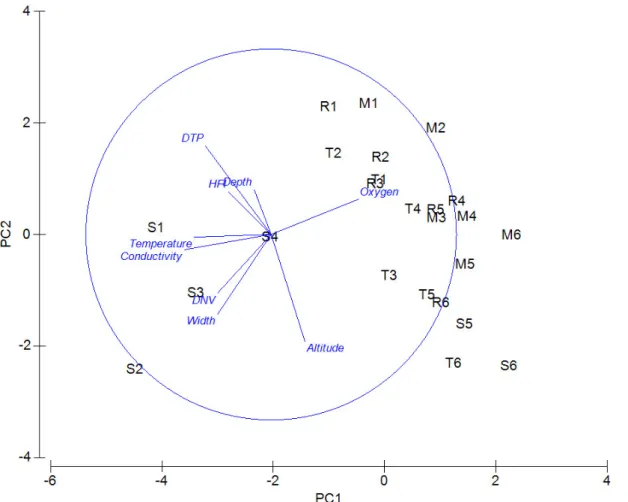
Results of the PCA using the abiotic data arranged the 24 sampling sites as shown in Figure 9. A distinction between S1, S2, S3 and S4 and all the other sites is clear. PC1 explain 38.1% of all variation and PC2 21.8% (Table S1 in Annex). The main abiotic factors responsible for the separation in PC1 were oxygen (positive direction), conductivity and temperature (negative
20
direction) as for the PC2 were altitude and width (negative direction) and DTP (positive direction) (Table S2 in Annex).
Figure 9 – Principal Components Analysis (PCA) showing the arrangement of the 24 sampling sites based on the abiotic factors measured. PC1 explains 38.1% of all variance and PC2 21.8%.
3.2 Macroinvertebrate communities
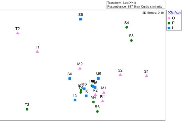
A total of 29710 individuals belonging to 90 taxa were identified.The MDS of the macroinvertebrate communities (Figure 10) shows a great similarity between all sites in Mente and Rabaçal Rivers as well as upstream sites in the Tuela (T4, T5 and T6) and Sabor (S6) Rivers. The other sites tend to be grouped according to spatial proximity: S1 and S2; S3 and S4 and T1 and T2, with T3 and S5 isolated from all others. Permanova results indicate that there are no significant differences in the macroinvertebrate communities between park status (Pseudo-F=1.1; p=0.3). Macroinvertebrate taxa sampled in this work are presented in Table S3 in Annex.
21
Figure 10- Multidimensional scaling (MDS) of the macroinvertebrate communities showing sampling sites and park status.
The SIMPER analysis showed that the taxa contributing the most to the average dissimilarity between outside and periphery (49.3%) were Oligoneuriidae (3.9%), Hydropsychidae (3.7%) and Caenidae (3.7%), while between outside and inside (46.7%) were Simuliidae (4%), Brachycentridae (3.7%) and Oligoneuriidae (3.6%) and between periphery and inside (43.2%) were Brachycentridae (4.3%), Oligoneuriidae (4.1%) and Simuliidae (3.9%) (see Table S4 in Annex).
Average (±SD) macroinvertebrate richness (number of families) was higher inside the park with 32.6 (±5.6) families present, followed in the periphery with 28.2 (±10.7) and lower outside with 27.4 (±6.6) (Figure 11A). However, ANOVA results showed no significant differences in macroinvertebrate richness between park status (F2,21=0.98; p=0.39). Sites S6, R3 and M3 were characterized by the highest richness, with 42, 40 and 38 different families present, respectively, and sites S1, S3, S4 had the lowest with 18, 16 and 11, respectively. Average (±SD) abundance of macroinvertebrates was higher inside the park with 1523.1 (±676.8), followed by the periphery with 1251.9 (±696.1) and lower outside with 938.8 (±812.2) (Figure 11B). No significant differences in macroinvertebrate abundance between park status were observed (F2,21=1.3; p=0.3). Sites S2, T6 and M4 hold the highest abundances with 2708, 2510 and 2494 individuals respectively, and T1, S5 and T2 the lowest with 448, 405 and 198, respectively. Average (±SD) Shannon-Wiener (H’) diversity was higher outside the park with 2.19 (±0.29), followed by the
22
periphery with 2.14 (±0.38) and lower inside with 2.06 (±0.34) (Figure 11C). No significant differences in H’ index between park status were detected (F2,21=0.29; p=0.75). Sites M2, R2 and M3 hold the highest Shannon-Wiener diversity of macroinvertebrates with values of 2.57, 2.56 and 2.53 respectively, and M5, S3 and S4 the lowest with 1.65, 1.61 and 1.50, respectively. Average (±SD) Pielou’s evenness varied between 0.67 (±0.06) outside the park, followed by its periphery with 0.66 (±0.06) and inside with 0.59 (±0.09) (Figure 11D). Again, results of the ANOVA test showed no significant differences between park status (F2,21= 2.15; p=0.14). Sites M2, T4 and T2 had the greatest evenness values with 0.78, 0.76 and 0.71 respectively, and M5, T5 with 0.49 and S6 with 0.45 had the lowest values.
Figure 11 – Richness (A), Abundance (B), Shannon-Wiener diversity (C) and Pielou’s evenness (D) of the macroinvertebrate communities outside (pink), periphery (green) and inside (blue) the park. White circles represent the average values. Boxplots show median values (central line), the range from the 25th to 75th percentile (box) and the largest and lowest value within 1.5 times interquartile range below and above the 25th and 75th percentile (whiskers) and dots represent extreme values.
A B
23
Results of the regression analyses are present in Table S5 in Annex. Richness varied significantly with five abiotic factors (temperature, oxygen, conductivity, width and HFI), abundance with two (temperature and DNV), Shannon-Wiener diversity with three (oxygen, conductivity and width) and Pielou’s evenness with none.
Results from the IBMWP index indicated that all sites located in Rabaçal, Mente and Tuela Rivers as well as S2, S5 and S6 have a very good water quality (score >100); sites S1 and S3 have a good water quality (score 61-100); and only S4 is classified as polluted (score 36-60) (Table 2). Average (±SD) IBMWP varied from 185.6 (±37.4) inside the park, 148.1 (±40.2) in the periphery and 157.8 (±66.1) outside (Figure 12A). ANOVA test showed no significant differences in IBMWP index between park status (F2,21= 1.23; p=0.31). Regarding average IASPT (±SD), it was greater inside the park with 5.99 (±0.40), followed by outside with 5.93 (±0.46) and periphery with 5.84 (±0.69) (Figure 12B). No significant differences were found in IASPT index between status (F2,21= 0.16; p=0.86). Sites T3, R1 and M2 were characterized by a higher IASPT score of 6.60, 6.52 and 6.46 respectively, and S5, S3 and S4 showed the lowest with 5.08, 4.86 and 4.72, respectively. Average EPT% (±SD) was greater in periphery with a 42.3% (±5.8%), followed by outside with 41.4% (±7.3%) and inside with 40.8% (±7.7%) (Figure 12C). No significant differences in EPT percentage between park status were detected (F2,21= 0.10; p=0.90). Sites S4, T6 and T5 showed the higher percentage of 54.5%, 50% and 48.3%, respectively, and T1, T2 and S5 the lowest with 33.3%, 26.9% and 26.1%, respectively.
Table 2 – Water quality index for all the sampling sites in Mente, Rabaçal, Tuela and Sabor Rivers. IBMWP quality scores: >100 – very good; 100-61 – good; 36-60 – polluted; 16-35 – very polluted; <16 – extremely polluted (after Alba-Tercedor and Sánchez-Ortega, 1988).
M1 M2 M3 M4 M5 M6 R1 R2 R3 R4 R5 R6 IBMWP 183 179 216 192 148 195 137 206 230 194 197 201 IASPT 6.1 6.4 6.4 5.8 6.2 5.9 6.5 6.2 6.2 5.9 6.2 6.1 EPT % 45.5 46.4 44.7 38.9 44.4 36.1 43.5 43.2 42.5 41.2 44.1 38.9 T1 T2 T3 T4 T5 T6 S1 S2 S3 S4 S5 S6 IBMWP 163 108 165 145 181 209 100 109 68 52 117 237 IASPT 5.8 5.1 6.6 6.3 6.5 6.1 5.6 5.7 4.9 4.7 5.1 5.9 EPT % 33.3 26.9 35.7 43.5 48.3 50.0 44.4 47.6 37.5 54.5 26.1 38.1
24
Figure 12 –IBMWP (A), IASPT (B) and %EPT (C) water quality indices outside (pink), periphery (green) and inside (blue) the park. White circles represent the average values. Boxplots show median values (central line), the range from the 25th to 75th percentile (box) and the largest and lowest value within 1.5 times interquartile range below and above the 25th and 75th percentile (whiskers) and dots represent extreme values.
Results of the regression analyses are present in Table S5 in Annex. IBMWP varied significantly with five abiotic factors (temperature, oxygen, conductivity, width and HFI), IASPT with two (oxygen and conductivity) and %EPT with none.
Bivalves were present in all the four rivers surveyed and four different species (i.e. Margaritifera margaritifera, Potomida littoralis, Unio delphinus and Anodonta anatina) were found. Margaritifera margaritifera was present in all sites surveyed on Rabaçal and Tuela Rivers and U. delphinus was also found in T2. In Mente River only M. margaritifera was found in sites M1 and M2. In the Sabor River M. margaritifera was not present but P. littoralis, U. delphinus and A. anatina were found
A B
25
exclusively in S1. A total of 94 freshwater mussels were found in S1, being 87 U. delphinus, 4 P. littoralis and 2 A. anatina.
Regarding the pearl mussel M. margaritifera, a total of 1222 individuals were found, from which 44.9% were found inside the park, 33.1% in the periphery and 22.0% outside. Table S6 in Annex shows the abundance of pearl mussels in each site.
Average (±SD) abundance was greater inside the park with 12.5 (±18.6), followed by the periphery with 8.3 (±15.9) and outside with 5.9 (±10.7) ind. CPUE (Figure 13). ANOVA results did not detect significant difference in pearl mussels abundance between park status (F2,21= 2.05; p=0.13). However, and if we assess possible differences in abundance inside each river the results are distinct. For instance, in Mente River individuals are only present outside the park (Figure 14A); no differences exist in Rabaçal River (Figure 14B) between the different park status (F2,21=0.55, p=0.58) but the Tuela River had higher abundance inside park (Figure 14C), with significant differences between park status in this river (F2,21= 33.77; p>0.001).
Figure 13 – Abundance (ind. CPUE) of pearl mussel Margaritifera margaritifera outside (pink), periphery (green) and inside (blue) the park. White circles represent the average values. Boxplots show median values (central line), the range from the 25th to 75th percentile (box) and the largest and lowest value within 1.5 times interquartile range below and above the 25th and 75th percentile (whiskers) and dots represent extreme values.
26
Figure 14 – Abundance (ind.CPUE) of the pearl mussel Margaritifera margaritifera on Mente (A), Rabaçal (B) and Tuela (C) Rivers in each site outside (pink), in the periphery (green) and inside (blue) the park. White circles represent the average values. Boxplots show median values (central line), the range from the 25th to 75th percentile (box) and the largest and lowest value within 1.5 times interquartile range below and above the 25th and 75th percentile (whiskers) and dots represent extreme values. Different letters indicate significant differences among status.
Average (±SD) length varied between 72.3 (±12.3) outside MNP, 69.9 (±12.1) in the periphery, and 67.6 (±11.5) mm inside the park (Figure 15); with significant differences detected between park status (F2,1228=14.68; p>0.001). Pearl mussel length is significantly different between park status in Rabaçal (F2,21=14.27; p>0.0001), and Tuela (F2,21=73.85; p>0.0001) Rivers (Figures 16A and 16B). In Rabaçal River, average length inside is significantly lower than from the periphery and outside the park. In Tuela River, average length outside is significantly higher than inside and in the periphery of the park. No relationship was found between pearl mussel abundance and its fish host, Salmo trutta, abundance (R= 0.45, F=3.02, p=0.11).
A B
C b
27
Figure 15 - Length (mm) of the pearl mussel Margaritifera margaritifera outside (pink), periphery (green) and inside (blue) the park. White circles represent the average values. Boxplots show median values (central line), the range from the 25th to 75th percentile (box) and the largest and lowest value within 1.5 times interquartile range below and above the 25th and 75th percentile (whiskers) and dots represent extreme values. Different letters indicate significant differences among status.
Figure 16 - Length (mm) of Margaritifera margaritifera in Rabaçal (A) and Tuela (B) Rivers in each site outside (pink), in the periphery (green) and inside (blue) the park. White circles represent the average values. Boxplots show median values (central line), the range from the 25th to 75th percentile (box) and the largest and lowest value within 1.5 times interquartile range below and above the 25th and 75th percentile (whiskers) and dots represent extreme values. Different letters indicate significant differences among status.
A B
a b c
b