Can pairing strategies be even more profitable? : a study on pairs trading for the U.S. Russel 2000 Index constituents

(1)

Can pairing strategies be even more profitable?

A study on pairs trading for the U.S. Russel 2000 Index Constituents

Supervisor: Professor Joni Kokkonen Student: Muhammad Hussein Abdul Satar

Lisbon – 10th of March 2014

Dissertation submitted in partial fulfilment of requirements for the degree of MSc in Finance, at the Universidade Católica Portuguesa, 10th_{of March 2014.}

(2)

2 Abstract

Pairs trading is considered as a profitable Wall Street strategy. We analyse the influence of K-Means clustering using EPS and book-value per share ratios on pairs trading returns in the formation period, before coupling pairs, while using 3 different ranking methodologies which include the one proposed by Gatev et al. (2006). We use data from the Russel 2000 index from January 2003 to the end of June 2013, on 3.711 stocks. We find that a strategy based on the orthogonal regression approach outputs an impressive 4.35% statistically significant average excess monthly return and a Sharpe ratio of 3.23 if the K-Means clustering is applied and 20 pairs are selected, which compares to the Gatev’s strategy holding -0.54% without clustering for the same sample. We also find that the orthogonal regression method outputs on average 94 b.p. higher monthly excess returns than the average squared deviation methodology and that using the Pearson correlation coefficient for ranking pairs outputs permanently negative returns, independently of the clustering and number of pairs. Likewise, we find that the profitability of the pairs trading strategy is not dependent on the utilities sector.

(3)

3 Table of Contents, Index of Figures and Tables

1. Introduction ... 4

2. Data and Methodology ... 8

2.1 Absolute Price Deviation Methodology ... 10

2.2 Orthogonal Regression ... 11

2.3 Pearson correlation coefficient ... 12

3. Workaround for Computational Issues ... 13

4. Empirical Results ... 14 4.1 Strategies Profits ... 14 4.2 Risk Characteristics ... 16 4.3 Trading Statistics ... 18 5. Conclusion ... 21 References ... 23

Figure 1 - Formation and Trading Period for the period from 2003 to June 2013 ... 25

Figure 2 - Trading Methodology for all strategies ... 26

Figure 3 - Orthogonal Regression (Total Least Squares) ... 27

Figure 4 - Cumulative Monthly Returns for the clustered and unclustered strategies and the Equity Premium ... 28

Table I – Monthly Excess Returns of Pairs trading Strategies ... 29

Table II – Equity Premium for Pairs trading Strategies ... 30

Table III – Systematic Risk of Pairs trading Strategy ... 31

Table III – Continued ... 32

Table IV – Monthly Excess Returns of Pairs trading Strategies... 33

(4)

4

1. Introduction

Every so often, investors exploit relative price inefficiencies to obtain above market returns. An investment approach initially applied by Morgan Stanley (1983) to profit from these inefficiencies is the pairs trading strategy1, whose trading activity begins when two correlated assets (e.g. stocks that hold similar technical or fundamental characteristics) deviate from their equilibrium. Whenever there is a deviation, this strategy will then bet in the price re-convergence of the two stocks. Therefore pairs trading exploit eventual inefficiencies in the law of one price, which would determine that price changes in similar stocks should behave in the same manner.

Available research has been strongly limited due to the proprietary nature of the field (see e.g. Do, Faff and Hamza (2006)), as the trading methodologies are not openly revealed. Advanced methodologies only emerged in the last decade following Elliot, Hoek, and Malcolm (2005) who provide an analytical framework to test the strategy, suggesting a mean-reverting Gaussian Markov chain model for the stock pair’s relative price deviation – defined as the spread-, and Gatev, Goetzmann and Rouwenhorst (2006) who find their pairs trading strategy yielded average annualized returns of 11% (out-of-sample analysis from 1962 to 2002) net of conservative transaction costs. However, Gatev et al. (2006) underlined that returns were decreasing in recent years due to an increased hedge fund activity and compensations to arbitrageurs for enforcing the law of one price. Moreover, the abovementioned papers are focused in the optimization of returns during the trading period2_{while few papers examine the best methodology to generate stock} pairs.

1_{Bhattacharya, Rahul. Risk Latte. August 28, 2011. http://www.risklatte.com/Articles/History/H01.php} 2_{Refers to the period where the Pairs are actually traded in the stock market; after the formation}

(5)

5 In correspondence, this thesis is designed to look for evidence on pairs trading’s profitability aiming to find the best methodology to rank pairs, re-examining the findings of Gatev et al. (2006) for the period between July 2003 and the end of June 2013, focusing in the U.S. Russell 2000 constituents.

We follow the detailed methodology proposed by Andrade, Pietro and Seasholes (2005) and comple the work done on the trading period by Busse, Falcão, Afonso and Satar (2013) during the Empirical Finance Course. Furthermore we aspire to enhance Gatev et al. (2006) findings by testing other analytical frameworks on pair’s formation: the Pearson correlation coefficient and the orthogonal regression (approach from Lhabitant (2006)). Lastly, we use fundamental data to cluster the stocks with similar characteristics, besides only constraining the sectors by Industry.

Lin, McCrae and Gulati (2006) developed a procedure using co-integration that integrates a minimum profit condition into the pairs trading strategy to prevent losses, as market events, poor statistical modeling and parameter estimation may diminish all potential profits. Besides describing a five-step procedure to identify suitable pairs for trading, Lin et al. (2006) also verifiy the statistical validity of their procedure with the help of simulation data and tested the practicality with actual data. The authors show that this minimum profit condition has no statistical significant impact in the profits, relative to an unprotected trading strategy.

Moreover, Mudchanatongsuk, Primbs, and Wong (2008) provide another analytical framework to model the relative price deviations between a pair of stocks as an Ornstein-Uhlenbeck - a mean-reverting process with a greater attraction when the deviation is further away from the center. The authors were able to obtain an optimal solution to their formulated problem in closed form and derived the maximum-likelihood estimation values for parameters. Their paper is rounded up with a numerical study using

(6)

6 simulated data proving that the strategy could yield a yearly return of 38% under continuous compounding.

Following the study by Gatev et al. (2006), Do and Faff (2010) re-examine and enhance the evidence on pairs trading. Extending their original analysis to June 2008, the authors are able to show that profits continued to decrease in recent years: falling from 1.24% per each 6-month period between 1962-1988 to 0.6% for 2003-2008. The authors defend that increasing hedge fund activity, due to computational progress3_{, is not a} reasonable explanation for this phenomenon but rather a lower reliability of price convergence strategies due to an increase in stock market volatility. This in turn implies that the law of one price might be working better than before for the long horizons required by the strategy: i) the stock’s relative price divergence tends to happen due to changes in the fundamentals which lead to a decrease in the number of profitable trades or ii) the relative price divergence is not enough to open new transactions which doesn’t allow to explore most opportunities. However, more than half of the pairs chosen by the authors were still profitable. Furthermore, the authors were able to identify most profitable portfolios by setting up different strategies with respect to industry homogeneity and historical relative price convergence rates.

In our paper, we find that mean excess returns (excess returns from the strategy in relation to the 1-month U.S. T-Bill) and equity premiums (the excess return from the strategy against the Russel 2000 Index) are in fact negative for the strategy proposed by Gatev et al. (2006) in the Top 5 and Top 20 portfolios in a committed capital setup and using the Russel 2000 index. This is not only an evidence of Do and Faff (2010) results but a confirmation that the price convergence strategies are even worse if we use a larger

3_{Hennessee Group, January 26, 2008 -}

(7)

7 sample that includes smaller sized companies. However, if stocks are selected according to their fundamental characteristics as well, the monthly equity premium is 4.1% and 1.2% for the Top 5 and Top 20 strategies, respectively. Furthermore, a ranking methodology based in the correlation coefficient outputs on average negative equity premiums and a methodology based in the orthogonal regression outputs returns superior to the Gatev’s strategy for the Top 5 and Top 20 pairs.

In the first part of this paper we will describe the data that was collected to compute the results and the methodology for a total of 12 developed strategies. A special section is settled to briefly explain the issues faced due to the inexistence of faster computing and processing devices and the ways used to overcome this challenge. In the second part we disclose the empirical results: firstly exposing the strategies results and then analyzing the risk characteristics of the pairs trading methodologies. Lastly we present the descriptive statistics and conclude the paper with further research proposals.

(8)

8

2. Data and Methodology

Daily stock price data are collected from January 2003 to June 2013 for companies belonging to the U.S. Russel 2000 Index from Bloomberg. Data are retrieved in a way to replicate reality in the finest way and therefore values are adjusted for normal cash dividends, abnormal cash dividends, spin-offs, stock-splits, stock dividends and bonus and right offerings/entitlements.

We do a workaround to consider changes in the Russel 2000 Index composition: we capture its composition in 3 different times: 2003, 2008 (middle of the sample) and 2013. The data is then intersected, giving a sample of 3.711 stocks. This approach reveals the Russel 2000 had dramatic changes through the sample in study.

Contrary to Gatev et. al (2006) we account for 6 sectors instead of 4: communications, energy, financial, technology, consumer non-cyclical, consumer cyclical, basic materials, industrial and utilities. This is a consequence of the more recent data we are using, allowing for a superior segmentation of the statistics.

Figure 1 shows that pairs are formed on a rolling-window basis over a 12-month period (formation period) and traded in the 6 months (trading period) following the formation, as suggested by Andrade et al. (2005). Accordingly, trading periods are computed every 6 months with the first one starting in January 2004 giving a total of 19 sample trading periods.

We implement a new constraining mechanism based on K-Means cluster analysis – Centroids Ranking –, where K is the number of clusters built. This will allow to test if higher returns can be obtained when compared to the Gatev et al. (2006) ranking methodology, which constrains stocks only by sector. According to Hongxin, Jie, Jin and Chen (2007), this model has never been applied for pairs trading.

(9)

9 The goal of this strategy is to use fundamental ratios and compare them across stocks in the same industry. The pairs with the lowest distances across the ratios in the same industry are clustered and pairs can only be formed inside each cluster. We use multiples known as the best in the literature to compare across stocks (see e.g. Liu1, Nissim, Thomas (2002)) namely the earnings per share, the book-value per share, the 1-year forward earnings per share and the 2-1-year forward earnings per share.

In Statistical terms, this algorithm will have to minimize the objective function Ω:

Ω = ∑ ∑ ‖x_ij− cj‖ 2 k i=1 k j=1 , (1) where ‖x_ij− cj‖ 2

is the Euclidian distance measure between a data point x_ij and the cluster centre c_j. We define the number of clusters, K=4 for simplicity and we use three distance measures that are defined below.

Prices, which include reinvested dividends are normalized taking the first day of the formation period as the base, i.e. the prices start on the basis of 1. Overall 12 strategies are tested:

A. Absolute price deviation with/without fundamental ratios (FR) clustering with Top 5 or Top 20 pairs;

B. Orthogonal regression with/without FR clustering with Top 5 or Top 20 pairs; C. Correlation coefficient with/without FR clustering with Top 5 or Top 20 pairs. To build conservative estimates, we have considered 1 basis point for transaction costs per each trade. Furthermore, investments are constrained by using committed capital, i.e. if 10 pairs are selected to be traded, the capital base is 10 USD for the whole trading period irrespective of entry and exit into pairs.

(10)

10 2.1 Absolute Price Deviation Methodology

Following Gatev et al.’s (2006) approach to test pairs trading, the normalized price of day one for every formation period is set equal to one. The subsequent normalized prices are then obtained by increasing or decreasing the normalized prices by the daily return as seen in equation 2.

Pnorm_T = ∏T (1 + r_t

t=1 ), (2)

where Pnorm_T is the normalized price of a stock at a time t.

Then, pairs are identified by ranking couples of stocks from lowest to highest based on the sum of squared deviations between the two normalized price series. For all formation periods, we select the Top 5 and Top 20 pairs with the lowest deviations for trading whereby this measure is defined to be D_TXY_{for a stock X and the trading partner}

stock Y. D_TXY _{= ∑} _(Pnorm t X_{− Pnorm} t Y₎2 T t=1 (3)

The opening of trades is based on a standard deviation metric: trades are opened when the normalized stock prices of a pair diverge by more than two historical standard deviations, based on a historical average derived from the difference of the two normalized price series in the formation period. Equation 4 shows this threshold value which we define to be TXY. TXY ₌ − + _{2 ∗ St. Dev. ∗ (Pnorm} t X_{− Pnorm} t Y_{) (4)}

As soon as stock prices converge again, i.e. the threshold of the normalized prices reach zero, trades are closed. As pairs can open and close several times during the trading period this method is followed the whole 6-month period. In the case a trade doesn’t close

(11)

11 before the end of the trading period, profits or losses of this trade are calculated at the end of the last trading day. Figure 2 illustrates the trading strategy.

2.2 Orthogonal Regression

Models like the co-Integration likelihood by Lin et al. (2006) assume a causal relation from a dependent value to an independent value and find the line of best fit by minimizing the deviations of the dependent value. However, according to Lhabitant (2006), this is not the best way to model a stock pair relationship – when regressing between two stock prices, a more realistic assumption is that the two variables are interdependent but without a known causal direction.

The orthogonal regression, or Total Least Squares (TLS), finds the line that minimizes orthogonal distances, as shown in Figure 3, rather than vertical distances – minimizing the sum of the squared stocks deviations, rather than just one of them.

Following the TLS methodology proposed by Teetor (2011) and after using Equation 1 to get the normalized price series, we use Equation 5 to compute the hedge ratio, denoted as β. Assuming we have stock X and stock Y and we are trading their spread, if we are long in one unit of X, we must know how many units of Y to sell short. That quantity is given by the β (hedge ratio).

Furthermore, we apply the augmented dickey-fuller unit root test to find if β = 1, i.e. we’d only need 1 unit of Y to sell short. We then select the pairs with the lowest p-values, as recommended by Alexander (2001). In other words, if the p-values are very low then the model is a stationary process for this pair.

s_t = x_t− βy_t, (5) where s_t is the relative stock price’s deviation at time t, β is the hedge ratio, and x_t and y_t are the prices for stock X and Y respectively.

(12)

12 The opening and closing of trades is based on the standard deviation metric described in the previous section.

2.3 Pearson correlation coefficient

After using equation 1 to get the normalized price series, we use the Pearson correlation coefficient as an alternative strategy to rank pairs of stocks: from highest to lowest correlation. For all formation periods we select to trade the most correlated Top 5 and Top 20 pairs in terms of equation 6 whereby this measure is defined to be C_TXY_{for a stock}

X and the trading partner stock Y.

C_TXY = ∑Tt=1(PnormXt−Pnorm̅̅̅̅̅̅̅̅̅̅̅̅)(PnormX tY−Pnorm̅̅̅̅̅̅̅̅̅̅̅̅)Y

√∑T (Pnorm_tX−Pnorm_{̅̅̅̅̅̅̅̅̅̅̅̅)}X 2 t=1 √∑ (PnormtY−Pnorm̅̅̅̅̅̅̅̅̅̅̅̅)Y 2 T t=1 (6)

The opening and closing of trades is based on the standard deviation metric referred in the chapter 2.1.

(13)

13

3. Workaround for Computational Issues

It is important to note these methodologies could not be easily implemented with a normal statistical software and computer. R and R Shiny were used to allow for quicker computation, but still 3.711 stocks needed to be analyzed and combined 2 by 2, leading to 6.883.905 pairs of stocks to be made for each strategy every 12 months. A top computer would take 2 weeks to properly output each strategy results with this sample, therefore the sample was always constrained by sector of activity to reduce the amount of combinations and after that we split each sector’s sample into 4 groups by alphabetical order on the stock ticker for the unclustered strategies. The clustered strategies have these groups made by the K-Means formula. Pairs are made only within each group and the ones with the best rankings are chosen to be traded out of the full sample.

(14)

14

4. Empirical Results

4.1 Strategies Profits

Table 1 presents the monthly excess returns over the 1-month t-bill risk free rate4 on the committed capital for the portfolios on the 3 strategies and the variations between a strategy that selects stocks by clustering them with EPS, 1 year Forward EPS, 2 year Forward EPS and Book-Value per Share (K) and a strategy that only clusters the stocks by sector (U).

In Panel A, the absolute price deviation methodology outputs an average monthly negative return for the unclustered strategies and positive returns for the clustered ones, showing a monthly average excess return to the risk-free of 3.64% for the Top 5 pair strategy. Unfortunately the t-statistics reveal that these results are not statistically significant suggesting that the basic pairs trading strategy is not profitable for the Russel 2000 dataset.

Regarding the Panel A’s excess return distribution information, it is clear that the standard deviation is higher for the portfolios with only 5 pairs revealing diversification benefits. This is also shown by the spread between the maximum and minimum monthly returns that is higher for the portfolios with less pairs.

In Panel B, the panorama is different in the sense that the orthogonal regression outputs positive and statistically significant returns for the clustered strategies reaching 4.53% per month for the Top 20 pairs (t-statistic = 3.23). On one side this shows the orthogonal regression is yielding right now better payoffs than the strategy proposed by Gatev et al. (2006) with the same pairs (20) that yielded 0.90% per month, but it also tells

4_{Kennet R. French Data Library}

(15)

15 that pairs can be chosen in a properly way if they are clustered by their fundamental characteristics: similar stocks will only diverge if their financials are significantly different.

The excess return distribution for the orthogonal regression reveals diversification benefits as well and lower spreads between the monthly return picks.

In Panel C, we rank pairs based on the correlation coefficient as algorithm – the negative results exhibit that this methodology is not at all good for pairs trading. Returns are always negative in the correlation coefficient strategies but only statistically significant for the Top 5 pairs unclustered with -1.27% (t-statistic = -2.05). In the excess returns distribution, the correlation coefficient maximums and minimums are not much spread out. This can be a consequence of the lower number of trades with this strategy caused by the effect detailed in the latter paragraph.

Overall it can be said that pairs trading’s results from the unclustered strategy with the Russel 2000 is worse than previous tests with CRSP data (474 stocks in the Gatev et al. (2006) paper) which yielded 0.784% vs -0.85% and 0.805% vs -0.54% for the Top 5 and Top 20 strategies respectively. This is not only consistent with of Do and Faff (2010) results but a confirmation that the price convergence strategies are even worse if we use a larger sample that includes smaller sized companies.

Nonetheless, the clustered strategies provide higher returns compared to the unclustered ones what is clearly confirmed by Figure 4, where it is invested equally on each clustered strategy and computed monthly returns for each of them; the same investment distribution is applied for the unclustered strategies. A 1$ investment would lead to a capital gain of 3.33$ with the clustered strategy and a 0.42$ gain for the unclustered one over the period of analysis.

(16)

16

4.2 Risk Characteristics

This section holds a comparison of risks associated with each pair trading strategy, proving that risks associated with pairs trading are significantly reduced with the usage of clustering.

Table 2 compares the returns of each strategy over the market (Russel 2000). Looking at the first two moments of the returns distribution in Table 2 it can be noticed that the average equity premium provided by the clustered strategies is superior to the S&P500’s by more than 2.6% for the Absolute Price Deviation and 4.4% for the Orthogonal Regression and only at the expense of a little increase of the standard deviation. The Correlation Coefficient monthly excess returns are negative for the 4 strategy variations.

Applying a broadly used risk-adjusted performance measure – the Sharpe ratio – which incorporates both described characteristics, we see the clustered strategies on A and B portfolios hold always a positive ratio that is more than twice as high for all cases. This result is in line with our previous results of superior performance of the clustered strategy. Still, one can argue that this outcome may be misleading, as the returns may present negative skewness (Gatev et al., 2006). However, for the clustered strategies and for this particular sample, returns are in fact positively skewed. This would, on the contrary, affect the Sharpe Ratio negatively. Besides, the bad performance of the unclustered strategies is clearly underlined by a negative or close to zero Sharpe Ratio.

Furthermore the monthly excess returns are regressed on the three factors of Fama and French (1996) plus the Carhart’s Momentum factor (1997)5_{that is added to check if} the returns we are obtaining for the strategies are correlated with the market motion.

(17)

17 Results are shown in Table 3. Primarily, by analysing the intercept of the regression, that stands for the strategy return over its benchmark, it can be seen that for both A and B trading strategies its value is positive but it is only statistically significant for the clustered strategies of the orthogonal regression. However, the intercept in the clustered strategies are significantly higher than the unclustered ones.

Regarding the market risk it can be seen that for all normal significance levels pairs trading is not influenced by the market-risk, as it is a market-neutral strategy. For the two remaining Fama-French risk factors (size and book-to-market) evidence shows exactly the same: for a significance level of 5%, none of the coefficients can be stated as being statistically different from zero, meaning that none of the strategies tested is exposed to these kinds of risk.

When it comes to the momentum factor the estimates are usually negative, as it would be expected since the strategy follows the opposite of momentum strategies because one is betting on the prices re-convergence after a deviation from the equilibrium. Moreover, this risk is the one that should be more related to a pairs trading strategy.

The coefficient of determination is plotted in the last row of Table 3, showing that only a very small portion of the excess returns of the pairs trading can be attributed to the usual risk factors, meaning that pairs portfolios are nearly factor-neutral. The reason that can explain this fact is that pairs are computed in a way that in an ex-ante approach should match up economic substitutes.

(18)

18

4.3 Trading Statistics

Table 4 summarizes the trading characteristics and composition of the pair’s portfolios in a similar fashion of what Gatev et. al (2006) and Do and Faff (2010) exhibited. Even though we account 1 basis point per transaction, this information is relevant for transaction costs as it evaluates the trading intensity of the strategies every month and gives an insight on which sectors it is focused.

For the clustered strategies on both the absolute price deviation and the orthogonal regression, the average price deviation for opening pairs is 5.09% and 3.94% for the unclustered ones, revealing a narrower gap for the unclustered strategy and eventually a close to optimal gap for the clustered strategies. A small increase in the deviation happens when the number of ranked pairs grow as a consequence of the decrease in the proximity of the securities leading to an increase in the standard deviation of the prices.

For the Top 5 strategies the number of pairs traded per month is below 1 for all the 3 types of strategies, revealing months without transactions. Increasing the number of pairs to 20, pairs are traded three times per month on average. Optimality of clustering is also revealed on this statistic: the clustered strategies trade on average 1.51 times per month while the unclustered trade 2.12 times per month – only the best pairs are chosen when clustering. The average number of round-trip trades per pair for the unclustered strategies is 0.31 while the clustered ones get 0.38, revealing again that pairs are not traded more than once per month, on average.

The second section of Table 4 shows information on the composition of the pairs portfolios regarding market capitalization and industry membership. Different size characteristics are observed across strategies A (absolute price deviation), B (orthogonal regression) and C (Pearson correlation coefficient). For the absolute price deviation

(19)

19 strategy the average stock in the Top 5 and Top 20 strategies belong to the 2nd decile6; in the orthogonal regression the average stock in the Top 5 and Top 20 strategies belong to the 3nd and 4th decile respectively while the correlation coefficient picks an average stock in the Top 5 and Top 20 strategies belonging to the 5nd_{and 6}th_{decile respectively. This} insight reveals size matters for profitability, because while the average squared deviation strategy choses mostly big caps and the correlation coefficient contains many small caps, the orthogonal regression holds both big and mid-caps, and the latest is the most profitable strategy.

The remainder of this section gives information about the sector weights for each of the 12 strategies. Surprisingly, the Utilities sector accounts for only 7% of the pairs traded, while Gatev et al. (2006) exposed a 71% ratio. This fact is eventually caused by the larger number of stocks and larger sector distribution where some stocks that could be considered as utilities are now considered in other categories; this also addresses the issue pointed out by the same paper on whether the pairs trading strategy was limited to the Utilities Sector. In fact, the financial sector weights for an average of 25% of trades followed by consumer-cyclical with 19% on consumer non-cyclical and 17.5% for consumer cyclical in the absolute price deviation and orthogonal regression strategies. for the correlation coefficient strategies, the consumer cyclical holds 22% of transactions and the industrial sector stays at 17%.

Overall it can be said that strategies A, absolute price deviation, and B, orthogonal regression, are closer in what concerns stocks selection and trading characteristics while the correlation coefficient outputs usually unclear outcomes, being the cause of its

6_{The lowest deciles include the larger sized companies and the highest deciles refer to the lower sized}

(20)

20 negative returns. The clustered strategies seem to hold close to optimal characteristics, allowing for higher returns.

(21)

21

5. Conclusion

We examined if the suggested pairs trading strategy from Gatev et al. (2006) is still profitable for the United States if the sample is enlarged by including smaller sized stocks and if new methodologies based on K-Means clustering with orthogonal regression and pearson correlation coefficient could yield higher above market returns.

We found that the basic strategy by Gatev et al. (2006) generates negative equity premiums for the Russel 2000 but positive equity premiums of 4.1% with 5 pairs and 1.2% with 20 pairs if we opt for clustering the stocks with fundamental data. This follow the evidence from Do and Faff (2010) results and a confirmation that the price convergence strategies are even worse if we use a larger sample that includes smaller sized companies. The positive results with the K-Means clustering as used in Lipinga et al. (2007) proves that profitability can be recovered in Pairs Trading independently of the chosen ranking methodology.

Important results are also obtained concerning the methodologies chosen, where the correlation coefficient always outputs negative equity premiums and the orthogonal regression clustered strategies earn on average 4.4% monthly equity premium, which compares to the 2.6% monthly equity premium given by the absolute price deviation clustered strategies.

Also worth to mention are the portfolios of pair’s composition that are only focused by 7% on average for the utility sector, while Gatev et al. (2006) reached a 71% value. This is a consequence of a different portfolio composition and industry segmentation in our sample.

Further research should be conducted to analyse the time-series composition of pairs trading portfolio allowing to understand the changes in industry composition on

(22)

22 both bull and bear markets. Focusing on other world markets and combining worldwide stocks while taking care of sovereign risks can also be an intelligent step towards a more efficient strategy.

Finally, it is critical to re-conduct these tests without any clustering at all with the help of more powerful computing devices.

(23)

23 References

Alexander, Carol, 2001. Market Models: A Guide to Financial Data Analysis. West Sussex: John Wiley & Sons Ltd.

Andrade, S., Pietro, V. and Seasholes, P., 2005, Understanding the Profitability of Pairs Trading, Journal of Economic Literature, February 2005

Chan, Ernie, 2008. Quantitative Trading: How to Build Your Own Algorithmic Trading Business (Wiley Trading)

Do, B. and Faff, R., 2010, Does pairs trading still work? Financial Analysts Journal, 66(4): 83-95.

Do, B., Faff, R. and Hamza, K., 2006, A new approach to modelling and estimation for pairs trading. In Proceedings of 2006 Financial Management Association European Conference, Stockholm, June 2006.

Elliot, R. J., van der Hoek, J. and Malcolm, W.P., 2005, Pairs trading. Quantitative Finance, 5(3):271-276.

Fama, E. and French, K., 1996, Multifactor Explanations of Asset Pricing Anomalies. Journal of Finance, 51: 131-155.

Gatev, E., Goetzmann, W.N. and Rouwenhorst, K.G., 2006, Pairs trading:

Performance of a Relative-Value Arbitrage Rule. Review of Financial Studies, 19(3):797-827.

Hongxing He, Jie Chen, Huidong Jin and Shu-Heng Chen, 2007, Trading Strategies Based on K-means Clustering and Regression Models

Lhabitant, François-Serge, 2006, Handbook of Hedge Funds (John Wiley & Sons, Ltd.) Lin, Y., McCrae, M. and Gulati, C. M., 2006, Loss protection in pairs trading through minimum profit bounds: a cointegration approach. Journal of Applied

Mathematics and Decision Sciences, Volume 2006 Art. No. 73803.

Mudchanatongsuk, S., Primbs, J.A. and Wong, W., 2008, Optimal pairs trading: A Stochastic Control Approach. In 2008 American Control Conference,

Washington, USA, June 2008.

Nath, P., 2003, High Frequency Pairs Trading with U.S. Treasury Securities: Risks and Rewards for Hedge Funds, Journal of Economic Literature, November 2003

(24)

24 Perlin, M. 2007, Evaluation of pairs trading strategy at the Brazilian financial market, Munich Personal RePEc Archive, MRPA Paper No. 8308, April 2008

Petras and Podlubny, 2010, Least Squares or Least Circles? A comparison of Classical Regression and Orthogonal Regression, Vol.23, Nº2

Teetor, Paul (2011), Better Hedge Ratios for Spread Trading (Unpublished working paper)

Yan-Xia, L., McCrae, M. and Gulati C., 2005, Loss protection in pairs trading through minimum profit bounds: a cointegration approach. Journal of Applied

Mathematics and Decision Sciences, Volume 2006, Article ID 73803, Pages 1-14, May 2006

(25)

25

Figure 1 - Formation and Trading Period for the period from 2003 to June 2013 This Figure was adapted from Busse et al. (2013) Empirical Finance paper where Formation Periods and Trading Periods are drawn in a way to allow continuous trading and rebalancing every 6 months. Each formation period has 12 months of data and each trading period has 6 months.

Time Formation period 1 Trading period 1 Formation period 3 Formation period 4 Trading period 3 Trading period 4 01/03 07/04 01/04 07/04 01/05 07/05 0 1/06 01/12 07/12 01/13 07/13 Formation period 19 Trading period 19 Formation period 2 Trading period 2

(26)

26

Figure 2 - Trading Methodology for all strategies

This Figure was adapted from Busse et al. (2013) Empirical Finance paper and applies to the trading period for all the 12 trading strategies presented in the paper. The Historical Average is the average price deviation during the 12-month formation period. Trades are opened the next day after the price reaches 2 or -2 standard deviations and closed when the prices return to the historical average or when the 6– month trading period ends.

Price

Divergence Price Divergence

+2*St.Dev. Historical Av. -2*St.Dev. Close e Open Month 6 Month 0

(27)

27

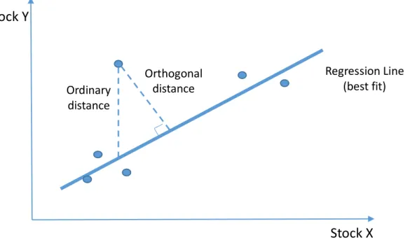
Figure 3 - Orthogonal Regression (Total Least Squares)

After computing the Regression Line, we don’t take the ordinary distance to study pairs co-integration, but yes the orthogonal distance that makes a 90 degree liaison between the stock Y or X and the best fit line.

Stock Y

Stock X

Orthogonal distance Regression Line (best fit) Ordinary distance

(28)

28

Figure 4 - Cumulative Monthly Returns for the clustered and unclustered strategies and the Equity Premium

This chart pictures the return out of 1$ invested in the clustered and unclustered strategies in January 2004 up to the end of June 2013. The investment is equally distributed in 6 equal parts for the clustered strategies and 6 equal parts for the unclustered ones. It is also pictures the Russel 2000 to analyze the equity premium. 0 0,5 1 1,5 2 2,5 3 3,5 4 4,5 5

jan/04 set/05 mai/07 jan/09 set/10 mai/12

P o rtfo lio va lue (1 $ inv es tm ent )

(29)

29

Table I – Monthly Excess Returns of Pairs trading Strategies

Pairs Portfolio K U K U

A. Average Squared Deviation

Average Excess Return (commited capital) 3,64% -0,85% 0,74% -0,54%

Standard error 0,02 0,01 0,01 0,01

t-statistic 1,69 -0,88 0,88 -0,82

Excess Return Distribution

Median 1,07% -1,44% 0,51% -0,19% Standard Deviation 23,03% 10,37% 8,96% 7,00% Skewness 0,38 -0,66 0,59 0,47 Kurtosis 4,61 10,00 3,42 2,45 Minimum -96,17% -56,24% -27,33% -18,45% Maximum 93,70% 44,52% 36,27% 30,31%

Observations with excess return <0 45,61% 56,14% 46,49% 52,63%

B. Orthogonal Regression

Average Excess Return (commited capital) 3,33% -0,37% 4,53% -0,72%

Standard error 0,02 0,01 0,01 0,01

t-statistic 1,85 -0,57 3,23 -1,26

Median 0,37% -0,90% 2,06% -1,08% Standard Deviation 19,24% 6,97% 14,97% 6,05% Skewness 1,19 0,64 1,26 0,65 Kurtosis 3,73 1,81 3,20 1,78 Minimum -41,75% -20,31% -28,92% -18,10% Maximum 80,18% 24,55% 66,64% 21,43%

C. Correlation Coefficient

Average Excess Return (commited capital) -0,85% -1,27% -1,27% -0,74%

Standard error 0,01 0,01 0,01 0,01

t-statistic -1,46 -2,05 -2,05 -1,11

Median -1,09% -1,58% -1,58% -0,45% Standard Deviation 6,23% 6,63% 6,63% 7,19% Skewness 0,54 0,01 0,01 0,11 Kurtosis 2,84 5,69 5,69 0,48 Minimum -21,29% -30,26% -30,26% -20,56% Maximum 22,24% 29,08% 29,08% 21,32%

Top 5 Top 20

Summary Statistics of monthly excess returns to the risk-free rate (1-month U.S. T-Bill) on portfolios of pairs between January 2003 and June 2013 (3,711 observations). The opening of pairs trading is delayed by one day to make the the backtesting more realistic. The "top n" profolios include the n pairs with least distance measures while K stands for stocks clustered by their fundamental characteristics and U for stocks not clustered on that measure. On Panel A are shown the Average Squared Deviation Strategies where pairs are ranked according to least distance in historical price space and therefore . Panel B results stand for the Ortoghonal regression where pairs are ranked from the lowest to the highest p-values. Panel C reports statistics on the Pearson Correlation Coefficient - pairs are ranked from highest to lowest correlation coefficient. The t-statistics are computed using the usual standard error. Absolute kurtosis is reported.

(30)

30

Table II – Equity Premium for Pairs trading Strategies

Mean Equity Premium 0,04098 -0,00398 0,01196 -0,00081

Standard deviation 0,24 0,11 0,11 0,09

Sharp Ratio 0,17 -0,04 0,11 -0,01

Semestral serial correlation 0,13 0,05 -0,16 0,00

B. Ortogonal Regression

Mean Equity Premium 0,03784 0,00081 0,04987 -0,00262

Sharp Ratio 0,20 0,01 0,31 -0,03

Semestral serial correlation 0,03 -0,09 0,38 -0,13

Mean Equity Premium -0,00396 -0,00820 -0,00100 -0,00290

Sharp Ratio -0,05 -0,10 -0,01 -0,03

Semestral serial correlation -0,13 -0,24 -0,14 -0,15

Top 5 Top 20

Mean Equity Premium is in excess of the Russel 2000 Index for the 12 strategies, between January 2003 and June 2013 (3,711 observations). The opening of pairs trading is delayed by one day to make the the backtesting more realistic. The "top n" profolios include the n pairs with least distance measures while K stands for stocks clustered by their fundamental characteristics and U for stocks not clustered on that measure. On Panel A are shown the Average Squared Deviation Strategies where pairs are ranked according to least distance in historical price space and therefore . Panel B results stand for the Ortoghonal regression where pairs are ranked from the lowest to the highest p-values. Panel C reports statistics on the Pearson Correlation Coefficient - pairs are ranked from highest to lowest correlation coefficient.

(31)

31

Table III – Systematic Risk of Pairs trading Strategy

(continued)

Pair Trading Portfolio Performance K U K U

Average Excess Return 3,64% -0,85% 0,74% -0,54%

Standard error 0,02 0,01 0,01 0,01

Sharp Ratio 1,69 -0,88 0,88 -0,82

Semestral serial correlation 0,13 0,20 -0,02 0,12

Factor model: Fama-French + Momentum

0,04850 0,00110 0,02049 0,00660 (0,01) (0,46) (0,01) (0,16) 0,00312 0,00317 -0,00316 0,00059 (0,3) (0,12) (0,09) (0,37) -0,01242 -0,00099 -0,00231 -0,00007 (0,13) (0,42) (0,29) (0,49) -0,00044 0,00447 0,00059 -0,00630 (0,48) (0,44) (0,44) (0,02) 0,00169 -0,00044 -0,00247 -0,00132 (0,36) (0,42) (0,09) (0,18) R2 0,01246 0,02020 0,03885 0,04089 B. Ortogonal Regression

Average Excess Return 0,033296 -0,003736 0,045329 -0,007165

Standard error 0,018020 0,006526 0,014017 0,005669

Sharp Ratio 1,85 -0,57 3,23 -1,26

Semestral serial correlation 0,04 0,11 0,50 0,11

0,04010 0,00700 0,05667 0,00367 (0,01) (0,13) (0) (0,25) 0,01011 0,00086 -0,00020 0,00057 (0,02) (0,31) (0,48) (0,35) -0,00657 0,00218 -0,00400 0,00216 (0,23) (0,25) (0,29) (0,22) 0,00284 -0,00262 0,00400 -0,00227 (0,36) (0,18) (0,27) (0,18) -0,00114 -0,00270 0,00030 -0,00242 (0,39) (0,03) (0,46) (0,02) R2 0,05469 0,05231 0,00630 0,05404 MOM Top 5 Top 20 Intercept Market SMB HML MOM Intercept Market SMB HML

(32)

32

Table III – Continued

Average Excess Return -0,00850 -0,01274 -0,01274 -0,00744

Standard error 0,00583 0,00621 0,00621 0,00673

Sharp Ratio -1,46 -2,05 -2,05 -1,11

Semestral serial correlation -0,13 -0,02 -0,15 -0,02

0,00140 -0,00162 0,00490 0,00449 (0,4) (0,4) (0,15) (0,25) 0,00452 0,00011 0,00212 -0,00179 (0) (0,47) (0,05) (0,17) -0,00174 0,00237 -0,00137 -0,00368 (0,27) (0,22) (0,28) (0,14) -0,00398 -0,00282 -0,00051 0,00479 (0,06) (0,16) (0,41) (0,06) 0,00050 -0,00170 0,00006 -0,00126 (0,34) (0,11) (0,48) (0,2) R2 _0,08225 _0,02503 _0,02647 _0,05246 HML MOM

Monthly risk exposures for portfolios of pairs formed and traded according to the "wait one day" rule discussed by Gatev et al. (2006), over the period between January 2004 and the end of June 2013. The four measures are the Fama-French factors and the Carhart's Momentum factor. Returns for the portfolios are in excess of the risk-free rate (U.S. 1 month T-Bills outputed from Fama-French Database). The P-Values are in parenthisis below the coefficients and follow the normal computation way.

Intercept Market SMB

(33)

33

Table IV – Monthly Excess Returns of Pairs trading Strategies

(continued)

A. Absolute Price Deviation

Average Price Deviation Trigger for opening pairs 0,05036 0,04558 0,05811 0,02875

Average number of pairs traded per month 0,85 0,91 3,04 3,84

Average number of round-trip trades per pair 0,26 0,24 0,62 0,36

Standard deviation of number of round trips per pair 0,34 0,34 0,28 0,12

Average Size Decile of stocks 2,23 2,75 2,96 2,98

Average Weight of Stocks in top three size deciles 0,74 0,78 0,78 0,79

Average weight of Stocks in top five size deciles 0,93 0,97 0,92 0,98

Average Sector Weights

Communications 0,11 0,14 0,11 0,13 Financial 0,32 0,25 0,30 0,24 Technology 0,07 0,05 0,08 0,05 Energy 0,02 0,04 0,01 0,01 Consumer, Non-Cyclical 0,17 0,18 0,18 0,21 Basic Materials 0,05 0,05 0,01 0,04 Industrial 0,05 0,03 0,03 0,04 Consumer, Cyclical 0,18 0,21 0,22 0,23 Utilities 0,03 0,05 0,06 0,05 B. Ortogonal Regression

Communications 0,10 0,08 0,11 0,05 Financial 0,21 0,23 0,22 0,25 Technology 0,03 0,09 0,04 0,07 Energy 0,04 0,08 0,02 0,09 Consumer, Non-Cyclical 0,21 0,19 0,23 0,18 Basic Materials 0,08 0,03 0,09 0,04 Industrial 0,03 0,13 0,03 0,14 Consumer, Cyclical 0,15 0,12 0,16 0,13 Utilities 0,15 0,05 0,1 0,05 Top 5 Top 20

(34)

34

Table IV – Continued

Communications 0,06 0,07 0,07 0,08 Financial 0,15 0,16 0,14 0,10 Technology 0,02 0,07 0,07 0,09 Energy 0,09 0,02 0,05 0,06 Consumer, Non-Cyclical 0,12 0,11 0,12 0,16 Basic Materials 0,04 0,06 0,09 0,12 Industrial 0,21 0,22 0,15 0,11 Consumer, Cyclical 0,3 0,25 0,18 0,14 Utilities 0,01 0,04 0,13 0,14

Trading Statistics and composition of portfolios of pairs between the beginning of January 2004 and the end of June 2013. Pairs are built over the 12-month period and traded over the subsequent 6-month period. The "top n" profolios include the n pairs with the best ranking results while C stands for stocks clustered by their fundamental characteristics and U for stocks not clustered on that measure.The Formation Period ranks depend on the implemented strategy as followed: On Panel A are shown the Average Squared Deviation strategy statistics where pairs are ranked according to least distance in historical price space and therefore ; Panel B results stand for the Ortoghonal regression where pairs are ranked from the lowest to the highest p-values; Panel C reports statistics on the Pearson Correlation Coefficient - pairs are ranked from highest to lowest correlation coefficient. In the trading period, trades are made according to the rule that opens a position in a pair on the day following the day on which the prices of the stocks in the pair diverge by two historical standard deviations. Information on the trading characteristics of a pairs strategy and about the size and industry memebership of the stocks in the various portfolios is given in the above panels. Average deviation to trigger opening of pair is the cross-sectional average of two standard deviations of the pair prices difference.