Deep Learning Applied to PMU Data in Power Systems

(1)

F

ACULDADE DE

E

NGENHARIA DA

U

NIVERSIDADE DO

P

ORTO

Deep Learning Applied to PMU Data

in Power Systems

Pedro Emanuel Almeida Cardoso

Mestrado Integrado em Engenharia Eletrotécnica e de Computadores Supervisor: Prof. Dr. Vladimiro Henrique Barrosa Pinto de Miranda Second Supervisor: Dr. Ricardo Jorge Gomes de Sousa Bento Bessa

(2)

(3)

Abstract

The analysis of power system disturbances is fundamental to ensure the reliability and security of the supply. In fact, capturing the sequence of system states over a disturbance is an increased value to understand its origin. Phasor Measurement Units (PMUs) have the ability to record these fast transients with high precision, by providing synchronized measurements at high sampling rates. Indeed, these events can occur in a few seconds, which hampers their detection by the traditional SCADA (Supervisory Control and Data Acquisition) systems and emphasizes the uniqueness of PMUs. With the advent of Wide Area Measurement Systems (WAMS) and the consequent deploy-ment of such monitoring devices, control centers are being flooded with massive volumes of data. Therefore, transforming data into knowledge, preferably automatically, is an actual challenge for system operators.

Under abnormal operating conditions, the data collected from several PMUs scattered across the grid can shape a sort of a "movie" of the disturbance. The importance of WAMS is therefore sustained on their ability to capture the sequence of events resulting from a disturbance, helping the further analysis procedures. Driven by the amounts of data involved, this dissertation proposes the application of Deep Learning frameworks to perform automatic disturbance classification. In order to do so, a set of measurements from several PMUs - installed in the Low Voltage grid of an interconnected system - is used, from which representative patterns are extracted so as to endow a classifier of knowledge related to system disturbances.

In particular, the strategies herein adopted consist of the application of Multilayer Perceptrons, Deep Belief Networks and Convolutional Neural Networks, the latter having outperformed the others in terms of classification accuracy. Additionally, these architectures were implemented in both the CPU and the GPU to ascertain the resulting gains in speed.

Index terms: Artificial Neural Network, Convolutional Neural Network, Deep Belief Neural Network, Deep Learning, Power System Disturbance Classification, PMU, WAMS.

(4)

(5)

Resumo

A análise de perturbações severas num sistema elétrico de energia é fundamental para assegurar a fiabilidade e segurança do fornecimento de energia eléctrica. Efetivamente, capturar a sequência de impactos decorrentes de uma perturbação constitui um passo importante para a determinação da sua origem. As PMUs (Phasor Measurement Units) têm a capacidade de registar estas vari-ações rápidas com elevada precisão, providenciando medições sincronizadas obtidas com elevada taxa de amostragem. Este tipo de eventos pode ocorrer em poucos segundos, o que dificulta a sua deteção através dos tradicionais sistemas SCADA (Supervisory Control and Data Acquisition), evidenciando as características únicas deste aparelho de medição. Com o advento dos sistemas de medição sincronizada - referidos na literatura anglo-saxónica como WAMS (Wide Area Measure-ment System) - e a consequente proliferação das PMUs, os centros de controlo veem-se inundados por uma quantidade infindável de dados. Por conseguinte, a transformação desses dados em con-hecimento, preferencialmente de forma automática, representa um desafio atual para os operadores do sistema.

Numa situação de funcionamento anormal do sistema, os dados fornecidos por diversas PMUs espalhadas pela rede configuram uma espécie de filme que ilustra a perturbação ocorrida. A im-portância dos WAMS é, então, aferida na capacidade que estes têm para capturar a sequência de eventos resultantes da referida perturbação, sendo uma mais-valia para análises posteriores. Decorrente da quantidade de dados envolvida, a presente dissertação propõe a aplicação de ar-quiteturas de Deep Learning para classificação automática de perturbações. Para tal, são utilizadas medições registadas por PMUs instaladas na Baixa Tensão, das quais são extraídos padrões repre-sentativos de forma a dotar um classificador de conhecimento relativo a perturbações do sistema.

Mais especificamente, as estratégias adotadas consistem na aplicação the Multilayer Percep-trons, Deep Belief Networks e Convolutional Neural Networks, tendo estas últimas superado as restantes em termos de precisão na classificação. Adicionalmente, as arquiteturas mencionadas foram implementadas não só no CPU mas também com recurso a uma GPU, de forma a avaliar as acelerações daí decorrentes.

(6)

(7)

Acknowledgments

I would first like to thank my thesis supervisor, Prof. Dr. Vladimiro Miranda, for the opportunity, constant motivation and cutting-edge ideas to steer this research in the right direction. A word must also be addressed to Dr. Ricardo Bessa, as co-supervisor, for his valuable contribution to the work developed.

I am also very thankful to all my friends who took part in this journey. It would not have been this good without you all.

A special word goes to Mariana, for being by my side everyday, providing me with unfailing support and continuous encouragement.

Finally, I must express my very profound gratitude to my parents, for their loving support throughout my years of study and through the process of researching and writing this thesis. This accomplishment would not have been possible without them.

Thank you.

Pedro Emanuel Almeida Cardoso

(8)

(9)

“Without data, you’re just another person with an opinion.”

W. Edwards Deming

(10)

(11)

List of Figures

1.1 Frequency variation resulting from a generator tripping, registered with a PMU sampling at 60 Hz (blue) and a traditional SCADA acquisition device sampling at

0.5 Hz (red) . . . 2

2.1 Phasor representation of a sinusoidal signal. (a) Phasor representation; (b) Sinu-soidal Signal . . . 7

2.2 Elements of a PMU [1] . . . 7

2.3 Measurement system hierarchy [1] . . . 9

3.1 Performance of learning algorithms on available data [2] . . . 16

3.2 An example of the typical architecture of an MLP: input layer, a series of n hidden layers and an output layer . . . 19

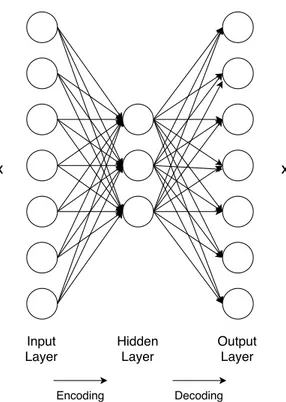
3.3 The structure of a classic Autoencoder. The network is trained to reconstruct the inputs x into x1_{, capturing the most salient features of the inputs in the smaller} dimension hidden layer . . . 21

3.4 Individual RBMs (left) can be stacked to create the corresponding DBN (right). For classification tasks, an output layer is also added . . . 22

3.5 Connectivity pattern between neurons of adjacent layers - how CNNs emulate the neuron response to stimulus only within its receptive field: units in layer m are connected to 3 adjacent units in layer m-1, therefore having receptive fields of width 3; the unit in layer m+1 is also connected to 3 adjacent units in layer m, therefore having a receptive field of width 3 with respect to that layer and a receptive field of width 5 with respect to layer m-1 (input) [3] . . . 23

3.6 Parameter sharing technique: the three units of layer m form a feature map and the connections of the same color are constrained to be equal (shared) [3] . . . 24

3.7 Architecture of the LeNet-5, a well-known convolutional neural network example [4] . . . 25

3.8 Hierarchical structure and signal flow of a DeSTIN architecture[5] . . . 26

4.1 Geographical disposal of PMUs implemented in Medfasee Project [6] - details in AppendixD . . . 30

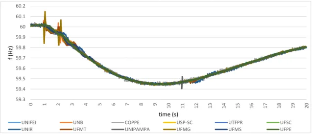
4.2 Typical frequency change in the presence of a Generation Tripping. Details about the PMUs that caught the event in AppendixD . . . 32

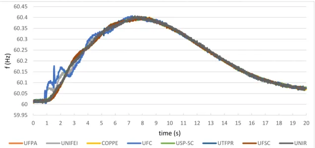
4.3 Typical frequency change in case of a load shedding - details in AppendixD . . . 33

4.4 Typical frequency change in case of a transmission line tripping off - details in AppendixD . . . 34

4.5 Typical frequency change in case of an oscillation - details in AppendixD . . . . 35

(16)

5.1 Generation Tripping: the input pattern of the CNN and the corresponding original frequency variation . . . 43

5.2 Load Shedding example: the input pattern of the CNN and the original frequency variation . . . 43

5.3 Line Tripping example: the input pattern of the CNN and the original frequency variation . . . 44

5.4 Oscillation example: the input pattern of the CNN and the original frequency variation . . . 44

5.5 CNN designed for performing classification in 30x40 images (adapted from [4]) . 45

5.6 Evolution of the training and generalization errors along with training epochs [7] 46

5.7 How the division of code sections is made between the GPU and the CPU [8] . . 47

(17)

List of Tables

1.1 Main attributes of traditional SCADA systems and PMU-based WAMS . . . 2

4.1 List of extracted events . . . 30

5.1 Specifications of the several Multilayer Perceptrons developed . . . 40

5.2 Specifications of the Deep Belief Network designed . . . 41

5.3 CNN settings defined for processing the input 30x40 and 20x60 images . . . 46

6.1 List of cases regarding each possible combination of 2, 3 and 4 events . . . 50

6.2 Accuracy of each architecture developed in each event distinction . . . 51

6.3 Predicted vs real events . . . 53

6.4 Speed-ups obtained with using the GPU: ratio time(CPU) / time(GPU) . . . 55

B.1 Hyper-parameters defined for the application of the 1 hidden layer MLP . . . 63

B.4 Hyper-parameters defined for the application of the Deep Belief Network . . . . 65

B.5 Hyper-parameters defined for the application of the 20x60 Convolutional Neural Network . . . 66

B.6 Hyper-parameters defined for the application of the 30x40 Convolutional Neural Network . . . 66

C.1 Accuracy obtained as a percentage of the total examples in each dataset . . . 67

C.2 Number of examples of each class in the dataset GT vs LS . . . 68

C.3 Number of examples of each class in the dataset GT vs LT . . . 68

C.4 Number of examples of each class in the dataset GT vs OS . . . 68

C.5 Number of examples of each class in the dataset LS vs LT . . . 68

C.6 Number of examples of each class in the dataset LS vs OS . . . 68

C.7 Number of examples of each class in the dataset LT vs OS . . . 68

C.8 Number of examples of each class in the dataset GT vs LS vs LT . . . 69

C.9 Number of examples of each class in the dataset GT vs LS vs OS . . . 69

C.10 Number of examples of each class in the dataset GT vs LT vs OS . . . 69

C.11 Number of examples of each class in the dataset LS vs LT vs OS . . . 69

C.12 Number of examples of each class in the dataset GT vs LS vs LT vs OS . . . 69

C.13 Confusion matrix for the MLP of 1 hidden layer applied to the dataset GT vs OS 70 C.14 Confusion matrix for the MLP of 1 hidden layer applied to the dataset LS vs OS . 70 C.15 Confusion matrix for the MLP of 1 hidden layer applied to the dataset LT vs OS . 70 C.16 Confusion matrix for the MLP of 1 hidden layer applied to the dataset GT vs LS vs LT . . . 70

(18)

C.17 Confusion matrix for the MLP of 1 hidden layer applied to the dataset GT vs LS

vs OS . . . 70

C.18 Confusion matrix for the MLP of 1 hidden layer applied to the dataset LS vs LT vs OS . . . 71

C.19 Confusion matrix for the MLP of 1 hidden layer applied to the dataset GT vs LS vs LT vs OS . . . 71

C.20 Confusion matrix for the MLP of 4 hidden layer applied to the dataset GT vs OS 72 C.21 Confusion matrix for the MLP of 4 hidden layer applied to the dataset LS vs OS . 72 C.22 Confusion matrix for the MLP of 4 hidden layer applied to the dataset GT vs LS vs OS . . . 72

C.24 Confusion matrix for the MLP of 8 hidden layer applied to the dataset GT vs OS 73 C.25 Confusion matrix for the MLP of 8 hidden layer applied to the dataset GT vs LS vs OS . . . 73

C.27 Confusion matrix for the DBN applied to the dataset GT vs OS . . . 74

C.28 Confusion matrix for the DBN applied to the dataset LS vs OS . . . 74

C.29 Confusion matrix for the DBN applied to the dataset LT vs OS . . . 74

C.30 Confusion matrix for the DBN applied to the dataset GT vs LS vs OS . . . 74

C.31 Confusion matrix for the DBN applied to the dataset GT vs LS vs LT vs OS . . . 74

(19)

Abbreviations

AE Autoencoder

AI Artificial Intelligence ANN Artificial Neural Network CI Communication Infrastructure CNN Convolutional Neural Network CPU Central Processing Unit dAE Denoising Autoencoder DBN Deep Belief Network

DeSTIN Deep Spatio-Temporal Inference Network DNN Deep Neural Network

FFNN Feed-Forward Neural Network GPS Global Positioning System GPU Graphics Processing Unit GT Generation Tripping LS Load Shedding LT Line Tripping

MLP i Multilayer Perceptron with i hidden layers NLL Negative Log-Likelihood

OS Oscillation

PDC Phasor Data Concentrator PLC Power-line Communication PMU Phasor Measurement Unit RBM Restricted Boltzmann Machine RMS Root Mean Square

ROCOF Rate Of Change Of Frequency SdA Stacked Denoising Autoencoder SGD Stochastic Gradient Descent

SCADA Supervisory Control and Data Acquisition SPDC Super Phasor Data Concentrator

UTC Coordinated Universal Time WAMS Wide Area Measurement System

(20)

(21)

Chapter 1

Introduction

This chapter presents a brief overview on the main topics addressed to in this work. It intro-duces the benefits resulting from the integration of Phasor Measurement Units (PMUs) in power system operation and the corresponding usefulness of Deep Learning as a computational tool for harnessing the resulting surplus of data.

The purpose and main contribution of the developed work are then described.

1.1 Motivation

Electrical Power Systems are dynamic infrastructures facing significant changes nowadays. The growth of decentralized energy sources penetration in the system is boosting the modifications required for improvements in both monitoring and control of power systems. The operation paradigm has changed, evolving from a load-driven to a generation-driven mode. That is, gen-eration is now leading the opgen-eration paradigm of power systems, since the increase of renewable energy sources leads to generation profiles that cannot be absolutely controlled. Therefore, a need arises for new solutions and technologies to improve the operation of the power system, with its growing complexity requiring more advanced and sophisticated monitoring capabilities.

Currently, transmission networks are endowed with more advanced solutions than distribution systems. In addition, the large presence of distributed energy resources connected at distribution levels is enhancing the role of this infrastructure in power system operation and emphasizing the lack of active distribution grids. The improvement of the monitoring resources for both transmis-sion and distribution networks is conceived as the employment of new measurement technologies and the development of new algorithms for data management. Phasor Measurement Units (PMUs) represent a significant upgrade in the measurement devices being used to improve the monitoring of power systems. Its uniqueness relies on providing measurements of both Root Mean Square (RMS) and phase of an electrical signal, with high sampling rates and synchronized with very accurate time-stamps provided by the Global Positioning System (GPS).

(22)

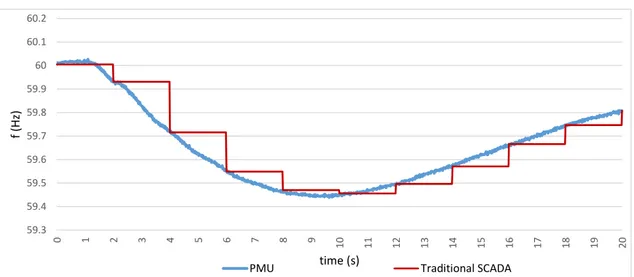
More specifically, PMUs provide 10-60 samples per second (10-60 Hz), which is very high when compared to the traditional SCADA acquisition devices that sample every 2-4 seconds (0.25-0.5 Hz). This significant difference is illustrated in Figure 1.1, where the frequency variation resulting from an actual generation tripping, registered by both technologies, is shown.

59.3 59.4 59.5 59.6 59.7 59.8 59.9 60 60.1 60.2 0 1 2 3 4 5 6 7 8 9 ₁₀ ₁₁ ₁₂ ₁₃ ₁₄ ₁₅ ₁₆ ₁₇ ₁₈ ₁₉ ₂₀ f (Hz ) time (s)

PMU Traditional SCADA

Figure 1.1: Frequency variation resulting from a generator tripping, registered with a PMU sam-pling at 60 Hz (blue) and a traditional SCADA acquisition device samsam-pling at 0.5 Hz (red)

It is evident that the adoption of PMUs can have significant impacts in the operation of the sys-tem. To better understand the resulting changes, a comparison between both paradigms regarding their main attributes is presented in Table1.1.

Table 1.1: Main attributes of traditional SCADA systems and PMU-based WAMS Attribute Traditional SCADA System PMU-based WAMS Resolution 1 sample every 2-4 seconds 10-60 samples per second Observability Steady State Dynamic / Transient Measured Quantities Magnitude Magnitude + Phase

Time Synchronization No Yes

Monitoring Local Global

By replicating several PMUs across the system and creating a Wide Area Measurement System (WAMS), the directly measured phasor data can help to infer the state of the power system, at a given instant, enhancing several control functionalities that the system operator has to deal with. So, PMUs are able to play a critical role in real-time operation, namely in stability surveillance throughout the electrical grid. The high precision knowledge PMUs can provide is required to minimize and control power outages and avoid problems such as cascading blackouts. This new paradigm results in a high resolution situational awareness, described perfectly by Terry Boston -CEO of PJM Interconnection, a USA region transmission organization - "It’s like going from an X-ray to an MRI of the grid.".

(23)

1.2 Main Contribution 3

Indeed, the time-synchronization of geographically dispersed measurements provides a better real-time operational awareness. This becomes particularly relevant in cases of abnormal operating conditions, in which the collection of measurements with high sampling rates captures the dynamic behaviour of the system, providing a deeper knowledge of the transients involved. Having the measurements duly synchronized, the sequence of grid states over an occurrence represents a kind of a "film" of the event, that can be reproduced and used for improving examination methods such as post-mortem analysis.

As PMUs are deployed in larger numbers, the transmission and distribution operators will need practical tools to efficiently deal with the arising amounts of data. Consequently, the im-portance of developing innovative methods for harnessing the data collected from PMUs becomes evident. Indeed, the workload imposed by the stream of data generated by those devices suggests the application of Artificial Intelligence (AI) methods. In particular, the recent interest in Deep Learning is partly due to the availability of large amounts of data and also the improvement of computational power. Driven by these assumptions, this dissertation suggests the application of Deep Learning frameworks to extract knowledge from patterns present in raw data generated by a real, PMU-based, measurement system.

1.2 Main Contribution

There is a willingness to bring closer the concepts of computer science and power systems, with the objective of using breakthrough strategies from the field of AI to leverage the way everyday problems of an electrical grid are solved. Since it is a very recent research subject, this dissertation represents a novelty with an added value for the state of the art of power systems.

The methodologies proposed intend to demonstrate how efficiently Deep Learning frameworks can perform on power system disturbance analysis, applied to a set of PMU measurements. The in-cursion herein conducted aims at developing disturbance classifiers based on the frequency change during a given occurrence - for instance, the one previously illustrated in Figure1.1. The distinc-tiveness of such an approach is to model the power system dynamics as a movie from which snapshots are taken and duly evaluated with the help of new computational tools.

In general, the main contributions are:

• Application of Deep Learning frameworks for extracting patterns from PMU frequency measurements: development of disturbance classifiers for post-mortem analysis;

• Performance evaluation of three classifiers: Multilayer Perceptron, Deep Belief Network and Convolutional Neural Network;

• Demonstration of the usefulness of Convolutional Neural Networks as a classifier on non-image data;

• Assessment of gains in the processing time of the methodologies proposed by harnessing the properties of GPU computing.

(24)

(25)

Chapter 2

Phasor Measurement Units

This is the first of two chapters reviewing the literature on the concepts related to this thesis. Here, the main features regarding Phasor Measurement Units are addressed. The chapter starts by pre-senting the basic concepts and moves towards the explanation on how PMU-based measurement systems are designed. Then, the most important subjects harnessing the data collected by the PMUs are described. The chapter ends with the incentive for the application of Deep Learning to PMU data.

2.1 Brief Overview

A Phasor Measurement Unit (PMU), which can be a dedicated device or as a function inte-grated in other devices such as protective relays, measures electrical waveforms in a power system, specifically voltage and current signals. Moreover, PMUs provide frequency and rate of change of frequency (ROCOF) of local measurements. With the use of a common time source provided by a Global Positioning System (GPS) clock, voltage and current measurements are time-stamped with high precision, enabling synchronization. This synchronized phasor measurements, also called synchrophasors, are becoming an important element of Wide Area Measurement Sys-tems (WAMS). Synchrophasors are enabling more advanced real-time monitoring, protection and control applications, therefore improving the electric power system operation.

2.2 Historical Background

The development of PMUs can be traced back to the field of computer relaying of transmission lines. The first works dedicated to transmission line microprocessor-based relaying (around the 1970s) were hindered by the insufficient computational capabilities to perform the calculations of all relaying functions. The research for reducing that computational effort came out with a solu-tion based on symmetrical component analysis of line voltages and currents [9]. The calculation of positive-sequence voltages and currents using the algorithms presented in 1977 [9] represented a great contribution for modern phasor measurement systems. Effectively, the importance and

(26)

applications of such an advent were identified in 1983 by [10]. These developments matched the beginning of the GPS project (1978), which offered the possibility of synchronizing measure-ments. In the early 1980s, the first PMU prototype using GPS was designed at Virginia Tech. However, the commercial manufacture of PMUs only started in 1991, in a collaboration between Virginia Tech and Macrodyne. This initiative and the further growth of PMUs manufacturers led to a series of "IEEE Standards for Synchrophasor Measurements for Power Systems" governing all issues related to phasor measurements.

2.3 Fundamentals of Synchrophasors

Charles Proteus Steinmetz, back in 1893, revolutionized the AC circuit theory and analysis when he introduced a way to describe a sinusoidal signal, using a complex number that referred to its RMS value and phase-angle - a phasor. The classical mathematical definition of a phasor can be depicted considering a sinusoidal waveform with constant frequency and magnitude, x(t):

xptq “ Xmcospwt ` φ q (2.1)

where Xmis the signal peak value, w “ 2π f is the angular frequency and φ the phase-angle of the signal. The corresponding phasor representation can be determined in both polar and rectan-gular coordinates, respectively:

xptq “?Xm 2e

jφ “ ?Xm

2pcosφ ` jsinφ q “ Xr` jXim (2.2) where the module of the phasor is the RMS value _?Xm

2 of the sinusoid waveform and Xrand Xim are the real and imaginary rectangular components of the complex phasor. Positive phase angles are measured in a counterclockwise direction from the real axis. However, phase is actually dependent of the initial time instant used as a reference, so it has to be referred correctly to that reference. Both phasor and sinusoidal representations are illustrated in Figure2.1.

Synchrophasors are as simple as synchronized phasors. More specifically, the phase-angle of a synchrophasor is calculated using the Coordinated Universal Time (UTC), provided by a GPS signal, as time reference. In doing so, a unique time reference is defined for all measured signals in a wide area, at a given instant, thus being synchronized.

2.4 Generic Configuration of a PMU

The purpose of a PMU is to provide phasor measurements of voltages and currents, clearly refer-enced to a time source, besides the additional frequency and ROCOF measurements. So, despite the existence of different manufacturers, a generic configuration of a PMU can be described and its

(27)

2.4 Generic Configuration of a PMU 7

Figure 2.1: Phasor representation of a sinusoidal signal. (a) Phasor representation; (b) Sinusoidal Signal

key elements are presented in Figure2.2. This structure is based on the first PMU built at Virginia Tech.

Figure 2.2: Elements of a PMU [1]

So as to compute positive-sequence measurements, all three-phase currents and voltages must be obtained from the respective current and voltage transformers. These can be acquired from several places in a substation and are identified as the analog inputs. To avoid aliasing errors, it is customary to use anti-aliasing filters, the frequency response of which is dictated by the sampling rate chosen for the sampling process. A common choice is to use analog-type filters with a cut-off frequency less than half the sampling frequency, meeting the Nyquist criterion [1]. Nevertheless, using a high sampling rate (thus oversampling) with a high cut-off frequency has some benefits. In fact, a digital decimation filter must be added so as to reduce the sampling rate, resulting in a digital anti-aliasing filter concatenated with the analog ones. In doing so, all analog signals have the same phase shift and attenuation, assuring that the phase-angle differences and relative magnitudes of different signals remain unchanged. Additionally, the oversampling technique can enable digital fault recording if raw data storage is available. It is important to note that current and voltage signals must be converted to appropriate voltages that match the requirements of the

(28)

analog-to-digital converters. The GPS receiver main task is to provide the UTC clock time used for time-tagging the sampled measurements. The phase locked oscillator converts the one pulse per second provided by the GPS into a sequence of high-speed timing pulses used in the waveform sampling. The microprocessor determines the positive-sequence of current and voltage signals. In phasor representations, the frequency of the sinusoidal signal is considered constant, implying stationary sinusoidal waveforms. Consequently, in practical applications where frequency does not remain constant, phasor representations must be handled carefully. This is usually surpassed considering the input signal over a finite data window, normally corresponding to one period of its fundamental frequency. Such a procedure can be conducted by several techniques depend-ing on the instantaneous system frequency. Since that frequency is seldom equal to the nominal frequency, the PMU must use a frequency-tracking step so as to estimate the period of the funda-mental frequency before the phasor is determined. Additionally, in order to do so, the PMU has to filter the input signal, separating the fundamental frequency from the harmonic or non harmonic components. The most commonly used technique for determining the phasor representation of an input signal relies on the application of the Discrete Fourier Transform (DFT) to a moving window over the sampled data. Considering N samples taken over one period and xk k “ 1, 2, ..., N ´ 1

( as the kth sample, the phasor representation is given by:

X “ ? 2 N ÿ xke´ jk 2π N _(2.3)

Finally, the output files of the PMU are transferred over the available communication facilities to a higher level in the measurement system hierarchy.

2.5 Measurement System Hierarchy

The architecture supporting modern measurement systems is commonly referred to as Wide Area Measurement System (WAMS). This term implies a set of new digital metering devices (e.g. PMUs), along with communication infrastructures, designed to acquire, transmit and process data over a wide geographic area.

Regarding PMUs as the quintessential example of metering devices, they are typically installed in power system substations. Despite local applications, the main use of PMUs information is carried out remotely at control centers. Therefore, a proper measurement system architecture is required, featuring, apart from the individual PMUs, dedicated communication channels and data concentrators. An illustrative scheme is shown in Figure2.3.

The PMUs provide time-stamped measurements of positive-sequence voltages and currents of all monitored buses and feeders in the respective substation, in addition to frequency and ROCOF. These measurements can be stored for further exploration, like post-mortem analysis. Since the lo-cal data storage is limited, relevant events are to be flagged for permanent storage. Besides storage,

(29)

2.6 Communication Infrastructures 9

Figure 2.3: Measurement system hierarchy [1]

a stream of information flows upwards being available for other applications. At a higher hierar-chical level, data from several remote PMUs is gathered in Phasor Data Concentrators (PDCs). The role of these devices depends on the application. For non-real-time scenarios, PDCs usually reject bad data and store all the information for future analysis. For real-time applications, such as network monitoring, PDCs align measurements according to each time-stamp. Subsequently, sorted measurements can be streamed to upper hierarchical levels such as control centers, where primary PDCs or Super Phasor Data Concentrators (SPDC) are placed. This hierarchical architec-ture enables information to flow from local to global entities.

The great advantage of such an architecture is that measurements coming from different sub-stations can be correlated in respect to the common time reference. Consequently, the status of a wide network-area can be directly obtained.

2.6 Communication Infrastructures

The deployment of a Wide Area Measurement System regarding Phasor Measurement Units re-quires robust communication infrastructures. In fact, real-time applications rely on the effective-ness of information flow between all elements of the measurement system. Therefore, commu-nication tasks should provide small latency - time lag between the instant of data creation and its availability for the desired application. In addition, an adequate channel capacity should be guaranteed, which is, in fact, rarely a limiting factor in PMUs applications.

Currently, optical-fiber is the physical medium of choice for communications, due to their unique channel capacity, high data transfer rates and immunity to electromagnetic interference [1], therefore meeting the requirements imposed. However, many existing applications are still using the conventional Power-line Communication (PLC) owing to its simplicity and low cost of implementation. Moreover, wireless infrastructures are emerging, with some applications using

(30)

the Internet via Virtual Private Network (VPN) systems. This is especially applied when large distances between the PMUs and the PDCs are involved, as seen in the Brazilian Synchronized Phasor Measurement System (SPMS) [11]. However, many existing applications are still using PLC.

With the advent of smart grids, significant investments are being made in the distribution grid, particularly in what regards the communication infrastructures (wired and/or wireless). This recent paradigm requires an almost absolute monitoring and control of the network, which is inherently dependent on the performance of the communication system. Therefore, it must be guaranteed a high level of robustness, with the infrastructure having some redundancy, high availability and speed, interoperability and security - especially cyber security, nowadays.

2.7 Output Data

The development of the synchrophasor technology and the corresponding need to transmit infor-mation over the network led to the establishment of several communication standards by the IEEE working group. Most recently, the IEEE C37.118-2 standard was developed, covering the com-munication framework and requirements for transmission of synchrophasors. Concretely, without imposing restriction on the communication media itself, the standard defines four file types for data transmission to and from PMUs:

• Header frame; • Data frame;

• Configuration frame; • Command frame.

The Header frame is the only human readable file, containing valuable information from the producer to the user of data. The Configuration frame is sent whenever the configuration of the system changes. Therefore, both Header and Configuration frame are transmitted by the PMU when the nature of data to be sent is defined for the first time. The Data frame, sent from the PMU to the PDC, contains the principal output of the PMU, such as the phasor measurements, frequency and ROCOF, voltages, currents, active and reactive powers. Finally, the Command frame is usually provided by higher levels of hierarchy for controlling the performance of the PMU (for instance, sent from a PDC to a PMU). Overall, under normal operation conditions, only the Data frame is communicated.

2.8 Harnessing PMU data

Synchronized phasor measurements are extremely important for monitoring and controlling the dynamics of a power system. Since PMUs were introduced into power systems in 1980s, their

(31)

2.8 Harnessing PMU data 11

value has been acknowledged by the extensive studied, proposed and implemented applications, which have shown significant benefits.

Nowadays, there are several PMUs installed around the world providing valuable information to improve power system operation. One of the major concerns regarding the deployment of PMU technology is its placement. Due to installation costs - devices, communication infrastructures and labouring - it is not cost-effective to install a PMU at every node of a system. That is why a great amount of research has been conducted to develop optimal placement strategies aiming at minimizing the number of devices. It is important to note that the intended applications of PMU installation are determinant to the strategies defined, with state estimation as one of the most common.

In [12], the authors present three different methods for optimal placement of PMUs: observ-ability factor analysis, sequential orthogonalization algorithm and coherency identification tech-nique combined with observability factor analysis. However, in addition to the cost of PMUs, the cost of the Communication Infrastructure (CI) has to be considered because it can even be dominant in relation to the cost of PMUs. Reference [13] shows that independent approaches for optimal placement of PMUs and optimal design of the CI might not lead to a global optimum so-lution in terms of cost; considering both simultaneously led to better soso-lutions in terms of cost and state estimation observability. In addition, a genetic algorithm is used for optimizing the defined problems, however exposing the methodology to the vicissitudes inherent of genetic approaches, such as randomness and computation effort. An extension to that work is proposed by [14], where binary imperialistic competition algorithm and Dijkstra algorithms are combined to optimize the cost of WAMS. Here, optimal placement of PMUs and CI design are determined simultaneously, whilst N-1 contingency is considered and observability is ensured.

Finding the optimum design of the measurement infrastructures to be installed is of great importance for power system operators. In fact, the development of modern WAMS is inherently dependent on the strategies found for PMUs placement, which have to be considered in investment plans. As aforementioned, the optimum solutions are dependent on the application to be explored. In general, there are five major areas of interest in which the PMUs have significant impacts [15]:

• Oscillation Detection and Control; • Load Modeling Validation;

• Voltage Stability Monitoring and Control; • System Restoration and Event Analysis; • Improvement on State Estimation; 2.8.1 Oscillation Detection and Control

The deregulation of electric power systems and consequent market-based scheme, along with con-tinuously growing demand, led to increasingly stressed operation in terms of oscillatory stability.

(32)

Therefore, the dynamics involved in power transmission became more complex, specially for low frequency oscillations. These are of great importance because they not only limit the amount of power transfer, but also degrade the power system security. The traditional SCADA systems can-not detect these fast dynamics due to their low data sampling rate and lack of synchronization. These restraints are effectively surpassed by the high data reporting rate of synchronized PMUs and the availability of fast communication links. So, the advent of PMU-based WAMS offers great opportunities to monitor the dynamic behaviour of power systems and identify its oscillation modes. For instance, an online monitoring of power system dynamics by using the synchronized measurements is presented in [16]. Additionally, both [17] and [18] suggest other online appli-cations, where Prony-based analysis - method used for the direct estimation of system modal in-formation - is implemented for frequency and damping oscillations detection by harnessing PMU data.

2.8.2 Load Modeling Validation

The analysis of a power system consists of modelling its various components and it has been an object of extensive studies. Thereof, load modelling has always been a challenging area for power system engineers, due to its great uncertainty and impact on system voltage and dynamic stability. In this practice, two approaches are widely employed: the component-based approach and the measurement-based approach [19]. The latter provides direct monitoring of true dynamic load variations, hence easily updating the load model parameters in real time for transient stability studies [20]. The recent growth of synchronized PMUs employment enhanced the efficiency of the measurement-based approach. In fact, the inherent accuracy of PMU measurements is reflected in the precision of load models, whereas the high reporting rates enable real-time development and validation of the model [21]. Moreover, [15] discusses the use of PMUs for measurement-based load modelling in the light of real-time security assessment and dynamic characteristics of end-use load.

2.8.3 Voltage Stability Monitoring and Control

In electrical power systems, voltage stability is inherent to the loadability of transmission net-works. Moreover, recent developments regarding distributed energy resources have brought in-creased uncertainty to power transfer as well as network expansion. Consequently, voltage stabil-ity has become a problem of major concern in both planning and operating of power systems. The advent of PMU technology brought the possibility of measurement-based real-time voltage sta-bility monitoring and control to transmission systems, thus improving the management of power transfer and system security [15]. For instance, [22] proposes an algorithm for voltage stability im-provement by optimally setting the output of control devices, assuming the availability of several dispersed PMUs. In a different perspective, [23] presents PMU-based Artificial Neural Network approach for faster than conventional real-time voltage stability monitoring. The synchronized

(33)

2.8 Harnessing PMU data 13

measurements are the inputs of the neural network, which is trained for providing the different voltage stability indices.

2.8.4 System Restoration and Event Analysis

Facing a major disturbance, system operators want to limit the resulting impact for consumers by restoring the system as quickly as possible. Afterwards, a complete event analysis must be driven in order to determine the root cause of the disturbance - commonly referred to as post-mortem analysis. However, the process of system restoration and event analysis is technically difficult to implement due to the absence of synchronized data and consequent computation time. Therefore, synchronized PMUs arise as a way to effectively deal with both issues.

As soon as a disturbance occurs, the protection system should detect it and operate appro-priately so as to isolate and minimize the affected area. Then, the location and source of the disturbance should be identified and isolated in order to restore power service. Approaches to fault location regarding PMUs reveal advantages in computation burden and technical assump-tions reduction [15]. In addition, [24] presents the effectiveness of high-speed synchrophasor data in a multi-terminal calculation of fault location.

As reported in [25], PMUs gave a significant contribution to information acquisition during a system islanding situation. The formation of the island was detected by monitoring the data from PMUs, where rapid diverging oscillations of frequencies were captured. Subsequently, [26] proposed a methodology for islands-synchronization with PMU measurements.

Overall, PMU-based systems can improve restoration time by providing high accuracy mea-surements that help pinpointing a fault. Also, the presence of synchronized data is greatly lever-aged whenever post-mortem analysis of events is required. These unique properties of PMUs also prospect a successful application in preventive recognition schemes.

2.8.5 Improvement on State Estimation

State estimation plays an important role in real-time monitoring and control of a power system. The traditional procedure uses measured voltage and current, real and reactive powers to infer the operating condition of the grid, at a given instant. The synchronized measurements provided by PMUs can be easily incorporated into state estimators along with conventional measurements [27]. Since voltage angles (which are state variables to be estimated in conventional state estimators) are measured directly, the accuracy of the state estimation is increased. This accuracy improvement was also obtained for dynamic state estimators [28].

State estimators are intended to provide the most likely state of the network. Therefore, they must be able to adequately detect and correct measurement errors, in a procedure called bad data processing. The detection of bad data in a power system can be improved by the effective place-ment of PMUs [29].

(34)

2.9 WAMS Implementations

Nowadays, Phasor Measurement Units are being used for several large scale WAMS implementa-tions around the world, from which some examples are mentioned.

In USA, The Bonneville Power Administration was the first electrical utility to implement a PMU-based architecture, in the beginnings of 2000. Thereafter, in response to the largest blackout in American history that affected about 50 million people in 2003, the New York Independent System Operator decided to install several PMUs in the system so as to prevent similar catas-trophic events [30]. In addition, Mexico developed a WAMS architecture capable of reaching up to eight transmission regions, helping the real-time monitoring and operation and improving sys-tem reliability and security [31]. China has also made substantial investments in this technology. Besides producing their own devices and standards, its grids have thousands of PMUs currently installed, mainly in EHV levels [32]. In Brazil, a phasor measurement project called Medfasee was developed. The project started by implementing Medfasee BT, a low voltage synchrophasor system in which PMUs are installed in universities. In 2013, 22 low voltage PMUs were already installed in several universities scattered around the country [6]. This brazilian project will be paid detailed attention in chapter4, since it provided a totally labelled dataset of disturbances recorded by the synchrophasor measurement system. Driven by the success of Medfasee BT, the Medfasee CTEEP was designed so as to implement a synchrophasor measurement system in a 440kV grid owned by CTEEP (Companhia de Transmissão de Energia Elétrica Paulista). In 2013, the project accounted 13 PMUs monitoring 13 transmission lines [33].

2.10 PMUs as a Big Data issue

With the advent of WAMS and the consequent the proliferation of digital measurement devices, control centers are being flooded with increasingly amounts of data. PMUs are capable of collect-ing samples at ratcollect-ings from 10 to 60 (dependcollect-ing on system frequency) samples per second [34], which are much higher sampling rates than the employed in traditional SCADA systems, that typ-ically collect measurements every 2-4 seconds [35]. This new paradigm represents a huge amount of raw data collected everyday. For instance, [36] refers that a single PMU sampling at 60Hz can create roughly 721MB of data per day. In addition, they use a dataset from Bonneville Power Ad-ministration’s PMU installation containing 44 PMUs that generate approximately 1TB per month. Reference [37] prospects how large-scale PMU systems present challenges for such a volume of data processing. Therefore, power system operators are craving for efficient techniques to digest the incoming data, improving grid operations. The volumes of data involved in the operation of WAMS suggest that this is a Big Data issue, where techniques in the field of Artificial Intelligence, like Machine Learning, can be very helpful to extract features from raw data.

(35)

Chapter 3

Deep Learning

This second chapter of the literature review describes the state of the art concerning Deep Learn-ing. After some initial considerations, the chapter addresses the concepts of learning from training and includes detailed description of the most important Deep Learning frameworks.

A section of final remarks regarding both chapters of the literature review can be found at the end.

3.1 Why Deep Learning?

Driven by the massive amounts of data involved in the operation of PMU-based WAMS, innova-tive methods in the field of Artificial Intelligence, such as Machine Learning, are emerging for harnessing the information provided and extract valuable knowledge for system operators. Instead of declaring complex analytical models, learning to recognize patterns and identifying features seems to be the answer to overcome the challenges imposed by processing the huge volumes of raw data involved in WAMS operation. Thus, as a class of the Machine Learning algorithms, Deep Learning arises as a computational learning technique in which high level abstractions are hierarchically modelled from raw data. In doing so, computers are taught to understand the world in terms of a hierarchy of concepts, where a complex concept can be defined in terms of simpler concepts. Why Deep Learning? The core of Deep Learning emergence lies on recent increase in computation power and access to enough data to train the algorithms. Also, in comparison to other learning algorithms, Deep Learning has shown better performance when larger datasets are involved. As illustrated in Figure 3.1, most learning algorithms reach a plateau in performance, whereas Deep Learning continues increasing.

The hierarchical learning representations of data in Deep Learning are usually inspired in neu-roscience, underlying the interpretation of information processing in neural systems. Hence, the majority of Deep Learning frameworks are based on the working principle of Artificial Neural Networks (ANNs), leading to the appearance of Deep Neural Networks (DNNs). DNNs can be considered as a class of ANNs where multiple hidden layers are placed between the input and output layers. Each layer is composed of single units, referred to as neurons due to the similarities

(36)

Figure 3.1: Performance of learning algorithms on available data [2]

they share with the behaviour of the neurons present in the human brain. Mathematically, a neuron can be considered as a non-linear function of the weighted sum of its inputs. This multi-layered processing enables the algorithm to learn representations from data with multiple levels of abstrac-tion. By composing the simple non-linear modules, representations at one level (starting from the raw input) are transformed into a representation at a higher, slightly more abstract, level [38].

3.2 Learning from Training

Learning from training is perhaps the most interesting property of ANNs. The ability of learning is generally obtained by iteratively adjusting the connection weights of neural network layers, so as to reproduce features of the input data. The theory of Machine Learning presents a broad categorization of its algorithms as supervised, unsupervised or even reinforcement learning, by the kind of experience they are allowed to have during the learning procedure.

In supervised learning, the algorithm experiences a dataset, in which each example consists of input values and the respective label/target. The outputs of the network are compared to the targets and the corresponding difference is determined. The weights are then adjusted so as to minimize such a difference. The backpropagation algorithm, addressed to in the following section, is considered the quintessential example of supervised learning.

In unsupervised learning, algorithms are fed with sets of unlabelled examples. The objective is to learn the probability distribution that generated the dataset. The connection weights are therefore adjusted by a self-organizing process that learns useful properties of the input dataset structure.

The algorithm can also be in a dynamic environment, receiving a reward feedback from its current performance, in a context of learning called reinforcement learning, which should not be confused with the supervised learning paradigm.

(37)

3.2 Learning from Training 17

3.2.1 Backpropagation

One of the most common and successful methods for supervised training of artificial neural net-works is the backpropagation algorithm. Introduced in 1986 by [39], the process adjusts the weights of the hidden connections of the network in order to meet a given loss function. This adjustment showed that backpropagation training is able to generate useful internal representa-tions of incoming data in the hidden layers of neural networks. A standard choice as the loss function is to minimize the difference between the actual and the desired output (for instance, the Mean Squared Error).

In general, the procedure comprises a two step sequence:

• Propagation — input data is presented to the network, propagating forward and producing an output. The output is compared to the desired/target values using a loss function that returns the resulting error;

• Weight Adjustment — the resulting error is then propagated backwards, updating the weights of the internal connections so as to minimize the loss function. This minimiza-tion is generally done through the applicaminimiza-tion of a gradient descent method, in which the weight parameters are iteratively updated in the direction of the gradient of the loss function, until the minimum is reached.

The latter step is the trickiest. Indeed, the accuracy of the model depends directly on how good the connection weights are adjusted. Time efficiency is also a concern, since this step can take a significant part of the training duration.

3.2.2 Gradient-based Optimization

The inherent nonlinearity of ANNs implies that most loss functions become non-convex. There-fore, these networks are usually trained employing iterative, gradient-based optimization methods, in order to conduct the loss function to the lowest value possible. Regarding a learning paradigm, objective functions are typically additive, formed as a composition of parcels from the training set, all summed up. Consequently, a gradient optimizer is also an additive operation. For this reason, optimizers have the possibility of performing one step (update of model parameters) based on two distinct techniques:

• Batch or Deterministic Gradient Descent — a single step requires running over the entire training set, hence updating the weights at the end of each epoch (one epoch is considered as a pass over all examples of the training set);

• Stochastic or Online — a single example is used at a time. The term Online refers to a specific case of real-time Stochastic, employed whenever each example is drawn from continuously created examples. The weights are updated after every training example until the entire training set is treated. At that point, an epoch of training is considered as complete, having performed as much updates as training examples.

(38)

In general, machine learning algorithms require large datasets for good generalization. Thus, applying the Batch Gradient Descent to huge training sets causes the time efficiency of the opti-mization to drop tremendously. On the other hand, the Stochastic Gradient Descent will imply a stochastic approximation of the true gradient of the loss function. In order to overcome those disadvantages, most applications employ a hybrid solution and use more than one example at a time -a mini-b-atch - inste-ad of -all the tr-aining set. This is commonly referred to -as Mini-b-atch Stoch-as- Stochas-tic Gradient Descent (SGD). Indeed, the Mini-batch SGD provides a more accurate estimate of the gradient [7] and is computationally more efficient in memory usage of modern computers [3], specially for GPU (Graphics Processing Unit) computing [7].

3.2.3 Problems with Training

The training process acquires additional importance to avoid common issues such as overfitting and excessive computation time. Frameworks like DNNs are prone to overfitting, that is, to over-adapt to the training set and lose capacity of generalization. In these cases, regularization methods such as dropout (where neurons are randomly removed during training, preventing the network from becoming overly dependent on any neuron) or early-stopping can be applied during training to help combat overfitting.

The success of backpropagation with stochastic gradient descent relies on its ease of imple-mentation and tendency to converge to better local optima than other methods. However, es-pecially for DNNs, these methods can be computationally expensive due to the many training parameters to be considered such as size of the network (number of layers, number of units per layer), learning rates and the initialization of weights. Covering all the parameter space to find the optimal parameters might not be feasible in terms of time or computation resources. This has led to several adaptations to speed up computation: mini-batching (determine the gradient for several training examples at once) and application of GPU computing.

In the development of the Deep Learning algorithms, both issues were considered and their solutions implemented. Therefore, these concepts are further detailed when appropriate - regular-ization in Section5.6.1, mini-batching and its influence on GPU computing in Section6.5.1.

3.3 Deep Learning Frameworks

Deep learning is a fast-growing field and new applications of its frameworks/architectures emerge often. The process of determining the best architecture is not straightforward, since it is not always possible or even advisable to compare their performance on the same datasets. That is, some architectures were developed for specific purposes and might not perform well on all tasks. Bearing that in mind, the following sections present a description of the most important Deep Learning Frameworks, especially for classification tasks (the aim of this dissertation). It is also important to note that Deep Learning has not come across the field of Power Systems very often, so the description given tends to be generic. Nevertheless, when appropriate, connections to Power Systems are traced.

(39)

3.3 Deep Learning Frameworks 19

3.3.1 Multilayer Perceptron

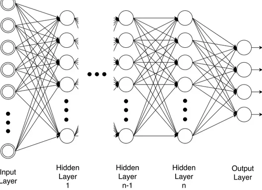
Multilayer Perceptron (MLP) is the name hereby given to a deep multilayered feedforward arti-ficial neural network, which is perhaps the most basic example of a Deep Learning Framework. The concepts related to structure and working principle of DNNs were continuously introduced as Deep Learning ideas were being introduced. So, to avoid redundancy, only the main features will be highlighted. In addition, an illustration of a typical MLP is given in Figure3.2.

Figure 3.2: An example of the typical architecture of an MLP: input layer, a series of n hidden layers and an output layer

Defining the structure of an MLP for a specific application can assume a high level of com-plexity. The number of neurons in the input layer is completely and uniquely determined once the shape of the input data is acknowledged. The output layer is specified by the aim of the solution developed. For instance, classification and regression require different but well defined output configurations. However, defining the number of hidden layers and respective number of neurons is not straightforward. Regarding the number of hidden layers, literature in general suggests that ore or two layers is usually enough and going deeper not always implies accuracy improvements. On the other hand, some rules-of-thumb for the number of neurons have been developed but are too generic for a universal acceptance - for instance restricting the number of hidden units to be between the number of units in the input and output layers. Still, these guidelines provide a starting point for a final selection based on trial and error.

(40)

Having defined the configuration and purpose of an MLP, its training is conducted in a super-vised fashion by employing the technique of backpropagation. If properly trained, these archi-tectures are able to acquire sufficient knowledge to solve its given task very accurately. In fact, they have shown very good performances in computer science field, such as speech and image recognition systems.

In what regards power systems, the application of ANNs in general, and MLPs in particular, is wide and not a novelty. Therefore, a lot of subjects have at least experienced their use: for instance, the definition of protection schemes for transmission lines, determining the location of the fault with ANNs [40] [41]; transformer fault diagnosis [42] [43]; on-line voltage stability mon-itoring [44]; forecasting problems of load [45] [46] [47], wind power [48] [49] and photovoltaic production [50] [51] [52].

3.3.2 Autoencoders

Autoencoders (AEs) are a kind of artificial neural network trained to output a copy of its input. However, it is usual to apply some restrictions that allow them to copy approximate and only inputs that resemble the training data. This process forces to prioritize given aspects to be copied, providing the ability to learn useful properties of data. Since merely copying the inputs may seem useless, the objective of training the Autoencoder is that the hidden layers obtain useful properties from data. A way of doing that is to constrain the hidden layer to have smaller dimension than the input layer, as exemplified in Figure3.3. This is a process commonly referred to as encoding, in which the Autoencoder is forced to capture the most salient features of the training data by representing it in an undercomplete representation, enabling dimensionality reduction [7]. Then a conversion of that representation is performed by a decoding function, retrieving the original format.

An interesting approach beyond the classic Autoencoders is found in the so-called Denoising Autoencoder (dAE). These can be interpreted as a stochastic version of the Autoencoder, receiv-ing a corrupted input ˜x and trained to reconstruct and obtain the original, uncorrupted input x. That is, firstly, a stochastic corruption process randomly chooses some of the input points and sets them to zero, simulating the removal of these components from the input [53]. This procedure approximates an actual issue affecting power systems nowadays, that being the case of missing data. Control centers are constantly flooded with measurements arriving from the various mea-surement points, and sometimes that information can be distorted or even missing. This could be explained by the malfunction of the metering devices or the communication facilities. In fact, this is a common issue regarding the communication of the measurements by PMUs. Receiving that sort of data values, the dAE tries to predict the missing/corrupted values from the non-missing ones. More specifically, the dAE encodes the input by preserving as many features as possible, followed by the inversion of the stochastic corruption effect applied to the input. Therefore, it aims at capturing the statistical dependencies between the inputs [3].

Stacked Denoising Autoencoders (SdAs) consist of series of dAEs forming a deep network, in which the output of one dAE is the input of the subsequent dAE. Such a framework is usually

(41)

Figure 3.3: The structure of a classic Autoencoder. The network is trained to reconstruct the inputs xinto x1_{, capturing the most salient features of the inputs in the smaller dimension hidden layer}

trained in an unsupervised, greedy (one layer at a time) fashion. Each layer is therefore trained as a single Denoising Autoencoder, focusing on reconstructing its input. Worth noticing in this case that greedy procedures are not always adopted. In fact, some alternatives regarding Infor-mation Theoretic and (top-down) Generative Model have been addressed to in both [53] and [3]. Additionally, as long as a classification task is desired, a second phase of supervised training is required. Slight adjustments are applied in this fine-tuning step, in which the network as a whole resembles an MLP.

3.3.3 Deep Belief Networks

The concept of Belief Networks is not new. In fact, their origin can be traced back to 1992 [54]. However, the depth of these and other architectures was not much explored due to the difficulty of training and consequent bad generalization performance. An explanation was found in the problems that randomly initializing parameters brought to gradient-based optimization [55]. The breakthrough for effectively train deep architectures was only introduced in 2006 by [56]: Deep Belief Networks (DBNs) are pre-trained in a greedy, layer-wise unsupervised manner, followed by a supervised fine-tuning process. More specifically, each layer is individually pre-trained with an unsupervised method, such as the Contrastive Divergence, for learning a non-linear transformation of its input. Afterwards, a gradient-based optimization performs the final supervised training

(42)

for fine-tuning the network. The unsupervised learning acts as an initialization of the network parameters by finding a good starting point in the parameter space for the supervised training, which represents better generalization [55]. Despite the initial eagerness, DBNs have been falling out of favour since they have been outperformed by other frameworks in several applications. Still, recent developments in power system forecasting research have reawakened the interest in DBNs, specially in the field of power systems, demonstrating its current usefulness and motivating the author to experience its performance.

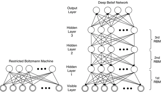
Structurally, DBNs can be understood as a composition of single unsupervised networks -Restricted Boltzmann Machines (RBMs) - stacked to form a deep architecture. As the name implies, RBMs evolved from the simple Boltzmann Machine, which is a fully-connected network with two layers, one visible and one hidden. By restricting the connections between neurons within the same layer, an RBM is created. The individual RBMs are stacked in a way that the hidden units of one RBM correspond to the visible layers of the next RBM. In doing so, the Deep Belief Network structure is generated, as seen in Figure3.4.

Figure 3.4: Individual RBMs (left) can be stacked to create the corresponding DBN (right). For classification tasks, an output layer is also added

In terms of structure, Deep Belief Networks are very similar to Multilayer Perceptrons. How-ever, the employment of RBMs and the distinctive unsupervised pre-training method turns DBNs into probabilistic generative models due to their ability to provide the joint probability distribution of their inputs and outputs. The additional supervised fine-tuning learning can be handled as in the traditional MLPs, requiring the provision of labelled data.

Mainly, DBNs have been used for generating and recognizing images [56] [57], video se-quences [58] and motion-capture data [59]. Moreover, Deep Belief Nets can also be structured so as to perform non-linear dimensionality reduction [60]. In fact, [55] showed that using Autoen-coders as an alternative to RBMs produced very similar results.

(43)

As mentioned earlier in this section, Deep Belief Networks have recently been employed in forecasting problems. For instance, [61] applied deep feature learning using DBNs for day-ahead wind speed forecasting. The DBN model employed was trained by using a step-by-step greedy algorithm, enabling the extraction of complex features of wind speed due to its strong nonlinear mapping ability, demonstrating high forecast accuracy. Moreover, applications in wind power forecasting regard a hybrid combination of Wavelet Transform and DBN, as adopted in [62] and [63]. Besides wind forecasting, in [64] a DBN is used for electricity load forecasting and the model implemented demonstrated good results in 24h ahead forecasting; in [65], a DBN is used for solar power forecasting.

3.3.4 Convolutional Neural Networks

Convolutional Neural Networks (CNNs) [4] are a special type of FFNN for processing data that has grid-like topology. Its structure is biologically-inspired, in which the connections between the neurons are based on the animal visual cortex. Each neuron responds to stimulus within their receptive field in a way mathematically approximate to a convolution operation. Receptive fields of different neurons partially overlap, tiling the visual field. Indeed, CNNs tend to explore spatially-local correlations, therefore enforcing spatially-local connectivity patterns between neurons of adjacent layers - a property sometimes called Sparse Connectivity. This special behaviour is illustrated in Figure3.5: the inputs of a hidden unit in layer m come from a subset of units in layer m-1 that are spatially contiguous (receptive field).

Figure 3.5: Connectivity pattern between neurons of adjacent layers - how CNNs emulate the neuron response to stimulus only within its receptive field: units in layer m are connected to 3 adjacent units in layer m-1, therefore having receptive fields of width 3; the unit in layer m+1 is also connected to 3 adjacent units in layer m, therefore having a receptive field of width 3 with respect to that layer and a receptive field of width 5 with respect to layer m-1 (input) [3]

Variations outside the receptive field of each unit do not interfere with its output. Thus, this architecture guarantees that the learnt "filters" produce an effective response to a spatially local input pattern. Stacking several layers, as shown in the previous figure, leads to "filters" that are more global, i.e., responsive to larger regions of the input space.

This connectivity pattern is replicated for all units within each layer to cover the entire visual field, which allows the detection of features regardless of their position in the visual field. In doing