Advanced impact integration platform for cooperative road use

Advanced impact integration platform for cooperative

road use

Jorge M. Bandeira

_{, Claudio Guarnaccia}

_{, Paulo Fernandes}

_,

_Margarida

C. Coelho

_*

a _{University of Aveiro, Centre for Mechanical Technology and Automation / Dep. Mechanical Engineering,}

Campus Universitário de Santiago, 3810-193 Aveiro - Portugal

b _{Department of Industrial Engineering, Faculty of Engineering, University of Salerno, Via Giovanni Paolo}

II, 132, I-84084 Fisciano (SA)

Abstract

In order to improve networks efficiency, a considerable number of studies has been addressing the potential of eco-friendly assignment solutions as alternative approaches to reduce emissions and/or fuel use. So far the majority of studies generally assumes that the most eco-friendly solutions are the ones that minimize the absolute amount of emissions produced along a certain trip. In this work a platform based on both empirical GPS data and microscopic simulation models of traffic, emissions, noise, and road safety was developed to examine in depth 4 routes of an origin-destination pair over a Portuguese city. In addition to the integrated externalities assessment based on state of the art techniques, a novelty of this work was the preliminary inclusion of social criteria in defining sustainable assignment solutions. This paper provides new insights about sustainable traffic management issues and addresses multiple novel route choice indicators. Specifically we found that the relative variation of the individual costs and total pollution produced among 4 routes varies to a factor of 1.4 while the variation of the potentially exposed population ranges up to a factor of 10. The main results confirm the need to take into account real-time urban activity patterns in order to effectively implement sustainable traffic management measures.

Introduction

In addition to traffic congestion, several transport-related negative externalities are known to lead to market inefficiencies and social welfare losses (Kickhöfer and Kern, 2015). Concerning environment, the transportation sector has the second biggest greenhouse gas emissions in the European Union (EU) EC, (2014). Road transportation contributes in more than two thirds of transport-related greenhouse gas emissions. Regarding local pollutants, there were substantial reductions, but emissions from road vehicles are still a main source of air pollution significant for human exposure. Approximately 75% Europe’s population lives in urban areas (UN, 2014) where exceedances of air quality standards often occur, causing serious health risks (EEA, 2013) and costs to society representing approximately 2% of the Gross Domestic Product (GDP) (United Nations, 2014). These results add to the evidence that long-term exposure to ambient air pollution is associated with increased mortality (Beelen et al., 2007; OCDE, 2014). In addition to air pollutants, noise emissions from road traffic are associated with various health outcomes (HEI, 2010). The external costs of noise (e.g. annoyance, health damage) in the EU amounts to at least 0.4 % of its GDP (NoiseInEU, 2015).

Liquid hydrocarbon fuels are expected to remain predominant over the next decades ((European Commission - EC, 2011). In this context, the White Paper for Transport 2011 emphasizes that advances in the automobile industry are not enough per se to minimize the above-mentioned problems. Thus, road networks must be operated in a way that maximizes positive impact on economic growth and minimizes negative impact on the environment. Hence, the efforts towards a more competitive and sustainable use of the transport networks need to consider the performance of the network under different domains and to bring an holistic approach to consider system performance, equity, and detailed assessment of external impacts.

1.1. Previous work on eco-assignment

In order to improve networks efficiency, since the last decade of the XX century, a considerable number of studies has been addressing the potential of eco-friendly assignment solutions as a way to reduce emissions and/or fuel use (Gwo-Hshiung and Chien-Ho, 1993). Different authors have been demonstrating empirically that a smart traffic assignment or proper route choice decisions may result in significant energy emissions savings. Boriboonsomsin et al., (2014) state that in future, where emission externalities are internalized in the form of carbon tax or else, the value of eco routes would be higher and financially attractive to drivers. Pereira et al., 2014 developed an eco-friendly app an based on GPS data and demonstrated that the routes defined by SmartDecision app can provide a 15%-32% reduction in health and social costs when compared with the recommended Google route. Empirical studies based on real world driving cycles data tend to be focused on individual impacts of a single vehicle (Bandeira et al., 2013; Frey et al., 2008; Minett et al., 2011) traveling on several routes, whereas analytical studies based on traffic simulation models are generally used for assessing the impacts of eco-routing strategies within the whole network (Ahn and Rakha, 2013; Ferguson et al., 2012; Guo et al., 2013; Levin et al., 2014). These methods conglomerate traffic and mobile-source energy and emission models with route minimization algorithms which are employed for routing proposes. Barth et al. (2007) applied such methodology in different case studies resulting in substantial fuel savings compared to usual navigation techniques. Zhang et al. (2010) addressed the air quality component as part of objective function of the optimization routing problem, but have emphasized that an alternative deserving further analysis is to contemplate air quality as a form of constraint to the optimization problem. However, research has also demonstrated that there are no single solutions to optimize all main traffic externalities (emissions, noise and safety issues) (Wismans et al., 2011). Furthermore, the major traffic

environmental externalities (noise and emissions) are seldom calculated in an integrated way (Wismans et al., 2013).

Additionally, a factor often neglected in network optimization algorithms is where the impacts are produced. So far the above mentioned studies generally assume that the best eco-route is the one that minimizes the absolute amount of a certain pollutant(s) emitted along a trip. Indeed, this approach is correct for greenhouse gases GHG (e.g. carbon dioxide – CO2) whose impact depend merely on the total quantity in the earth’s atmosphere.

However, there is a considerable number of traffic related externalities (local pollutants, noise and safety) which their effective impact is totally dependent on where they are produced. Conversely, the above mentioned previous studies on eco-navigation systems tend to implicitly presume that every unit of produced emissions is equally harmful. Recently, to overcome this drawback Kickhöfer and Kern, (2015) developed a simplified approach aiming at internalizing air pollution exposure costs, i.e. pricing damages to human health in an agent-based transport model with activity-based demand. However, there is still a lack of research addressing this issue in a context of smart and eco navigation systems.

For the assessment of traffic externalities, field data or the output of traffic simulation models can be used in combination with so-called effect models. It is not part of the scope of this paper to conduct an integrated review of these methodologies. However, comprehensive review works on this matter such as (Wismans et al., 2011) for integrated externalities platforms; (Hughes et al., 2015) for road safety (Smit et al., 2008) for pollutant emissions and (Garg and Maji, 2014; Guarnaccia, 2013) for traffic noise can be found. Overall, there is no consensus regarding a particular type of model that is the most appropriate or more valuable. Throughout the text we will try to rationalize the chosen approach for each analyzed dimension.

1.2. Study objectives

What has arisen from the literature on smart and eco navigation systems is that there are considerable advances in the development of solutions towards the optimization of driver’s costs and even on the minimization of total emissions. However, there are still research gaps in the field of internalizing traffic related effects and assessing more effectively social impacts. Massive and passive data such as cell phone density could provide detailed data on city activity patterns therefore contributing to identify the most vulnerable zones. This information could change the way how traditional routing systems are built and how the overall transport system is managed.

This paper aims at bringing new insights and new study variables towards the implementation of more effective eco-friendly and sustainable routing systems taking into account the fundamental pillars of sustainability – Social, Environmental, and Economic (see Fig.1). The analysis is based on a case-study and performed taking into account the different users of the transport network ecosystem: individual drivers (who choose the route); other drivers sharing the same routes; pedestrians and residents/workers potentially affected by the route choice.

The social aspect of sustainability focuses on balancing the needs for drivers with the needs of the society. Considering the social component we will focus primarily on all citizens (sharing the same roads whether drivers or simply residents and pedestrians) that can potentially be adversely and directly affected by the traffic volume increment.

Regarding the environmental component, the likely absolute impacts generated by route choice (pollutant emissions and noise) will be estimated.

The economic component will consider the monetary impacts associated with the cost of travel time along each route. Furthermore this pillar may be used to outline traffic assignment strategies that stimulate the utilization of socio-economic resources to their best advantage. A cost-effective route choice is more likely to remain stable and continue to be chosen over time.

The interaction of these layers result into new variables (equity, viability and bearableness) that can be applied for traffic management purposes. Thus, the main objective of this paper is to identify potential trade-offs among the parameters analyzed for a set of alternative routes. This paper provides the following novel contributions:

 Extension of the concept of “eco-routing” to “sustainable routing” or sustainable traffic assignment;

 Integration of different traffic-related externalities (noise, emissions and road safety) in the context of route choice decision process;

 Use of detailed GPS data to predict noise and pollutant emission and microscopic simulation to generate safety and route performance indicators.

2. Methodology

2.1. Overall methodology

A set of indicators was defined to evaluate the parameters of sustainability related to route selection (see Fig. 2). Indicators “A” refer to parameters usually taken into account for individual route choice decision: travel costs and more specifically travel time and fuel use (Boriboonsomsin et al., 2014). Additionally, an indicator based on the expected number of conflicts was developed. Indicators “B” and “C” are related to the environmental impacts of the route selection. This field includes criteria pollutants (B1-B3 – Carbon Monoxide (CO), Nitrogen Oxides (NOX) and Volatile Organic Compounds VOC) and noise emissions (B4)

whose major impacts are mostly generated at local scale and GHG (C1) – CO2, a global scale

externality (C1).

Indicators “D” and “E” refer to the impacts assessment of the route choice process, but considering the point of view of the remaining drivers sharing the same routes. For this purpose, environmental and delay performance functions were developed taking into account the local fleet characteristics (Fontes et al., 2014).

The indicators “F” and “G” are a first approach to include the vulnerability and social risk associated to route choice. At this stage, the link-based activity patterns (e.g. the exposed population living/working within a certain distance of the road) are determined based on empirical observation (videotaping) and geostatistical data.

Fig. 2 Overall methodology for developing route indicators. 1 _{Please Consult Bandeira et. al}

2013 and 2 _{Fontes et al 2014 for further description of the field work and the microscopic}

modeling platform validation)

2.2. Field work assessment of route choice impacts – individual perspective

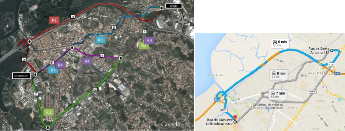
To analyze a set of sustainability indicators related to route choice decision, four routes located in the medium-sized Portuguese city of Aveiro were selected. All routes connect the northeastern part of the suburbs to the city center and all of them are alternatives suggested by traditional navigation systems (e. g Google Maps, via Michelin). These routes allow the

assessment of roads with different characteristics including a wide range of geometric configurations (arterials, motorways, and urban streets) and traffic conditions. In this case, we simulate up the impacts of route choice of a gasoline passenger vehicle travelling from the suburbs to the city centre in the morning rush hour (8:15-9:15 AM). This paper takes advantage of an extensive database (1200 km) of second-by-second GPS data collected in the city of Aveiro in previous research (Bandeira et al., 2013).

Travel time and emission results are based on a selection of GPS database recorded at 1 Hz rate over the four different routes. A sub-sample of GPS data was selected to analyze trips carried out during working days, at peak hour and without rainfall in the years 2011, 2012, 2014 and 2015. In total, 321 km of recorded GPS data were considered which corresponds to an average of 16 trips on each route. During this time interval (2011-2015) no structural changes in the network configuration were observed.

Travel time data (indicator A1), speed and acceleration data (1 Hz) were gathered directly from the GPS data logger. Altitude data was obtained through a Digital Elevation Model (Space Shuttle Radar Topography Mission 1) based on the geographic coordinates (GPS Visualizer). Due to the inexistence of significant obstacles (e.g. High buildings in narrow streets), for 99% of cases, the horizontal dilution of precision (HDOT) was within 2 m. 2.3. Travel time and total amount of air emissions produced

An instantaneous emissions model was used to estimate emissions. According to different authors, this type of models tend to be more realistic than average speed models (Coelho et al., 2013; Folberth et al., 2006) and especially in the context of comparative analysis of different routes (Ahn and Rakha, 2008; Bandeira et al., 2014; Frey et al., 2008). The methodology used to estimate emissions was based in the Vehicle Specific Power (VSP) which is built on regression models and allows characterizing the vehicle activity data on a second-by-second basis. The VSP values were categorized in 14 modes (ranging from -2 to

over 39 kW/ton) of the engine regime and an emission factor for each mode is used to estimate CO2, CO, NOX and Hydrocarbon (HC) emissions from an EURO 4 Gasoline

Passenger Vehicle (GPV) with engine size of 1.4 l which is a common vehicle observed in the local fleet (ACAP, 2012). Therefore typical vehicle activity data observed among the 4 routes of the study domain were characterized by instantaneous VSP obtained as (eq 1):

𝑉𝑆𝑃 = 𝑣[1.1𝑎 + 9.81 𝑠𝑖𝑛 (𝑎𝑟𝑐𝑡𝑎𝑛 (𝑔𝑟𝑎𝑑𝑒) + 0.132] + 0.000302 × 𝑣3 ₍₁₎

Where

VSP = vehicle specific power (kW/ton); v = velocity (m/s);

a = acceleration (m/s2_).

Instantaneous VSP was calculated for each trajectory observed among the four routes. The average number of seconds in each VSP mode (considering all runs in each route) was multiplied by the respective modal emission rate, and summed over all modes, to obtain total emissions of the trajectory performed on each route (eq. 2). Emissions rates for each VSP mode can be found in Coelho et al., (2009).

𝑅𝐸𝑖 = ∑14𝑖 𝐸𝐹𝑖𝑗×𝑡𝑖𝑗 (2)

Where:

REi = Total emissions of the pollutant i generated on route (g);

EFij = Emission factor for the source of pollutant i (NOX, CO2, CO, HC) for the VSP mode

j (1, 2, 3…14) (g/s);

Figure 3 presents the study routes. A KML interactive map data file is available to provide geospatial data information on the empirical tests for route driving cycle assessment. This file includes raw data of a representative trip performed over the 4 routes (instantaneous speed, acceleration, VSP, and VSP mode).

Route 1 is mostly performed on a motorway in free flow conditions (segment a) with an average traffic flow of 1400 vph at morning peak hour. This route goes into the city through the segment b, a single lane urban street operating near its maximum estimated capacity at 948 vph.

Route 2 is mostly performed in national roads (segments c and d) with 1-2 lanes per direction and with an average traffic flow of 1750 vph, corresponding to approximately a V/C ratio of 0.8. A mix of land uses types is observed along this corridor. The northern sections are predominantly commercial/industrial (segment c). Some agriculture fields can be found in the center while the southern d segment mostly consists of residential/services areas). Some recurrent traffic congestion is observed when approaching the 3 lanes roundabout located at the intersection of segments c, d and e and over the intersections of segment f, (two-lanes urban arterial).

Route 3 is virtually performed in urban arterials with a high density of residential and services areas (g and h segments). Although the average observed traffic flow in these segments (750 vph) is lower than in the former routes, this route is operating near its maximum capacity which is mainly constrained by the high density of intersections and traffic lights present in the urban core (Estimated V/C ratios: segment g-0.95 and h 0.75).

Finally route 4 is coincident with route 2 at segment c and with route 3 and segment d. Additionally, route 4 uses the segment e, (two lanes arterial) operating far from its estimated capacity (V/C of 0.6).

Fig. 3 Left: Aerial Map of the analyzed routes including second-by-second GPS logs for each route (Base map from Google Earth). Right: Snapshot of Google Maps suggestion for the analyzed Origin-Destination (OD) pair.

2.4. Noise assessment

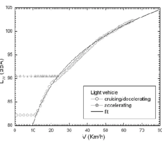
The evaluation of noise impact is commonly performed through the evaluation of the collective noise produced by a certain number of vehicles, in a certain time range, at a certain distance (see for example Guarnaccia et al., 2011; Iannone et al., 2013). In this section, the approach is somewhat different since the authors are interested to the noise level produced by a single vehicle, as one of the pollutants produced by the vehicles itself during the trip. For this reason, the authors developed the “Mean Noise Value” (MNV) produced by a vehicle and propagated to a certain distance. Thus, the steps that were followed are described below:

1) Evaluation of the source power level, as a function of the speed, both in cruising/decelerating and accelerating phases (gathered from GPS data);

2) Evaluation of the mean value of the source power level (log average), both in cruising/decelerating and accelerating phases;

3) Propagation of the source power level to a fixed distance from the vehicle.

Regarding point 1, the first choice is to follow the approach of Lelong (1999) in which the experimental power levels have been fitted as a function of the speed. In particular, for a light vehicle in cruising/decelerating state, the function is given by eq. 3:

{

82 𝑓𝑜𝑟 𝑣 < 11.5 𝐾𝑚/ℎ

(3)

with α = 53.6 ± 0.3 dBA and β = 26.8 ± 0.2 dBA .

In accelerating state, the sound level suddenly rises from zero to a constant value of 90.5 dBA, approximately until v = 25 km/h. Over this value, it switches to the curve of cruising/decelerating state (as shown in Fig. 4).

Fig. 4 Average Lw dependence from vehicle speed

Further methods to evaluate the source power level as a function of the speed can be implemented and compared in future work. For instance, the Imagine Model (Peeters, 2007) can be implemented, including the various coefficients that take into account many parameters (such as asphalt typologies, road gradients, accelerating and decelerating states). Also the “Common Noise Assessment Methods in Europe” (CNOSSOS-EU) model

(Kephalopoulos, Stylianos Paviotti and Anfosso-Lédée, 2012) could be considered, but both of these models have straight reference conditions such as constant vehicle speed, flat road, etc., that are not suitable for the approach of this paper. The approach presented here is a first approximation, enough coherent with literature, that allows the authors to have a reliable and simple formulation, for instantaneously emitted power source levels. Once the source power level formula has been obtained, the noise emission in each time step can be calculated and averaged over time. Let us underline that the mean value of the source power level is obtained performing a log average (eq. 4):

𝐿

̅

[

∑

] (4)

Finally, the propagation to a fixed distance is done according to the pointlike source propagation formula (eq. 5):

𝐿𝑃 = 𝐿𝑊− 20 𝑙𝑜𝑔

(

𝑟₀

)

In order to have a safe and precautionary approach, the authors will consider the asphalt as completely reflective (even if it is not). So, considering a reference distance r0 of 1 m, the

propagation formula to be adopted is given by eq. 6: 𝐿𝑃= 𝐿𝑊− 20 𝑙𝑜𝑔(𝑟) − 8 (6)

The chosen distance is 7.5 m, according to many regulations and papers in literature (see for instance (Bühlmann et al., 2015; Shilton et al., 2015) and the resulting value represents the mean value of the noise level “immitted” at 7.5 m , by a vehicle running on a certain route. The term “noise level immitted” stays for the noise level that instantaneously occurs

at 7.5 m when the vehicle is operating. Naturally, the average performed on the entire trip time range, has the meaning of the average noise level on the route.

2.5. Safety Indicator

The VISSIM microsimulation traffic model is widely accepted as a powerful instrument for perform an operation analysis of urban routes since it can be calibrated to set faithful representations of the traffic, assessments in urban areas (PTV, 2005). Furthermore, VISSIM permits exporting second by second trajectory files which in turn can be the input of external emission models. The simulation model was run for 90 minutes (7:30-9:00) with the first 30 minutes used for a warm-up period and data was extracted only for the remaining 60 minutes (8:00-9:00). Once this modeling platform has been calibrated and validated in a previous study, we suggest to consult the calibration and validation procedure in (Fontes et. al 2014)

For the safety assessment methodology, the software Surrogate Safety Assessment Model – SSAM was employed. This approach automates traffic conflict analysis by processing vehicle and pedestrian trajectories. For each interaction between vehicles using the same route, SSAM stores the trajectories of vehicles from the traffic model and registers surrogate measures of safety determining whether or not that interaction satisfies the condition to be deemed a conflict. Time-to-Collision (TTC) was used as a threshold to define if a given interaction is a conflict while the Relative Speed (DeltaS) was used as an indirect mean for the crash severity. TTC is the minimum time-to-collision value observed during the interaction of two vehicles on collision route. If TTC drops below a given threshold (1.5 seconds, as suggested for vehicle-vehicle events (Gettman et al., 2008) the interaction is tagged as a traffic conflict. DeltaS is the difference in vehicles’ speeds as observed at the instant of the minimum TTC (Gettman et al., 2008). Specifically, this value is

mathematically defined as the magnitude of the difference in vehicle velocities such that if v1 and v2 are the speed vectors of the first and second vehicle respectively, then DeltaS = ||

v1 – v2 ||. If they are traveling in the same direction and same speed then DeltaS = 0. If they

have a perpendicular crossing path, DeltaS = √2v. If they are approaching each other head on, DeltaS = 2v. SSAM categorizes subsequent conflicts into three categories based on a conflict angle (from -180° to +180°). The angle is expressed in the perspective of the first vehicle arriving at the conflict point, and indicates the direction from which the second vehicle is approaching relatively to the first one. The type is classified as rear end if 0º < conflict angle < 30°, a crossing conflict if 85º < conflict angle < 180°, or is otherwise a lane change conflict (Gettman et al., 2008). Due to the nonexistence of an updated database on road accidents in those routes, this method should be seen as a provisory road safety indicator that should be validated after the development of such crashes records.

2.6. Assessment of route choice impacts on other drivers

The route choice has not only direct influence on emissions produced by a given vehicle but also contributes, even if only marginally, to modify the performance of other vehicles using the same route, since the vehicles’ dynamics and interactions change.

To assess this effect, the previously described integrated traffic-emission microsimulation platform integrating the microscopic traffic simulator VISSIM and the instantaneous emission model VSP was used. The impact on route performance as a consequence of the route selection decision is based in terms of travel time (TT) variation, CO2 (global pollutant

and directly related to fuel use) and criteria local pollutants (NOX, CO, HC). To aid in

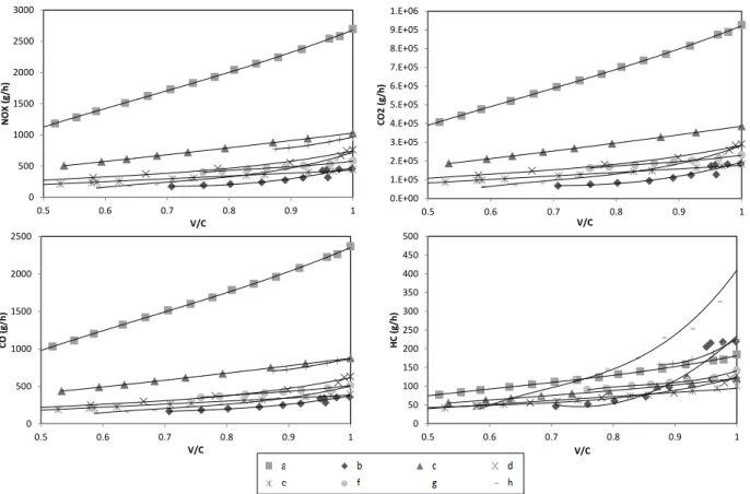
visualizing this concept a set of link-based relationships between volumes and traffic related externalities was developed. Volume-Delay-Functions (VDF), Volume-Emissions-Functions (VEF) (see Fig. 5) were expressly designed for each main segment of the network (see segments a, b, c, d, e f, g, and h, in Fig. 3). These relationships use the traffic volume as an

independent variable, and travel time (VDF) and emissions (VEF) as dependent variables. In this study, we use the average traffic volumes data during peak hour to assess the variation in route performance before and after an individual route choice. In the first scenario, all vehicles with a similar OD pair to the current study were removed from the simulation. Then multiple incremental traffic demands scenarios (20 vph) were performed, until the segment capacity is achieved. For each scenario 10 random seed runs were executed (Hale, 1997).

By conducting a regression analysis, a cubic polynomial function was shown to be appropriated to interpolate the traffic volume with total emissions produced over the analyzed segments (R2 _{> 0.95, p-value < 0.05). Fig. 5 illustrates these equations. It is}

expected that in near future these equations can be included into innovative online eco-assignment algorithms. For the purpose of this paper, these relationships will be used for establishing an indicator of relative impact on traffic performance associated with route choice.

For each parameter the marginal impact of choosing a certain route is given by (eq. 7)

𝑅𝐼 (%) =∑ 𝑓(𝑞+1)𝑛𝑖 −∑ 𝑓(𝑞)𝑛𝑖

∑ 𝑓(𝑞)𝑛 𝑖

(7)

Where:

RI – Relative impact on a certain route due to the marginal increment on demand; f(q) – Volume emission/delay function estimation for q vehicles per hour before assignment;

f(q+1) – Volume emission/delay function estimation for q vehicles per hour after assignment.

Fig. 5 VEF (NOX, CO2, CO and HC) for the analyzed network segments (a-h)

2.7. Assessment of route choice impacts on pedestrians, residents and workers (G and H) In addition to consider the absolute amount of route choice impacts, in a context of sustainable routing, it is essential to assess key characteristics of the routes to characterize the magnitude of the generated impacts. At this stage of the work, a qualitative assessment of the number of potential citizens that may be directly affected by a certain route choice was performed. The objective of this assessment is not to have a definitive answer on the exposure levels to traffic-related externalities, but rather to identify potential trade-offs between the minimization of traffic related impacts and the density of population directly affected by traffic externalities with strong and direct effect at the very local scale (e.g. CO, NOX, and noise emissions).

0 500 1000 1500 2000 2500 3000 0.5 0.6 0.7 0.8 0.9 1 N OX (g/h ) V/C 0.E+00 1.E+05 2.E+05 3.E+05 4.E+05 5.E+05 6.E+05 7.E+05 8.E+05 9.E+05 1.E+06 0.5 0.6 0.7 0.8 0.9 1 CO2 (g/h ) V/C 0 500 1000 1500 2000 2500 0.5 0.6 0.7 0.8 0.9 1 CO ( g/ h ) V/C 0 50 100 150 200 250 300 350 400 450 500 0.5 0.6 0.7 0.8 0.9 1 H C (g/h ) V/C

The Indicator F is related to the potential number of affected pedestrians. This indicator was developed based on videotaping performed during empirical work for traffic monitoring (see section 2.2). For each trip the number of pedestrians sharing the sidewalks of each route segment was counted in the lab by the research team. The indicator G corresponds to the mean value of pedestrians counted during 6 trips at morning peak hour.

The indicator H is related to the built environmental density and therefore indirectly related to the potential affected residents and workers that live/work on buildings which its façade is within 50 m of the center of the road. This distance is frequently used in risk assessment studies to traffic effects (Beelen et al., 2007; Finkelstein et al., 2004; Hoek et al., 2002). In order to determine the density of the built environment of the routes analyzed, the area of façades faced for the each route segments was determined according to eq. 8 and based on geo spatial data (CMA, 2015). These indicators based on “proximity” ignore the parameters that affect pollutants dispersion and physicochemical activity but are a reliable indicator of the potential exposure to traffic related impacts at the local scale.

𝐴𝑏 = ∑ 𝐵𝐻𝑃 − 𝑎𝑙𝑡𝑖𝑡𝑢𝑑𝑒 ∗𝑛𝑖 𝑙𝑒𝑛𝑡ℎ𝑖 (8)

Where

Ab = Area of building façades faced at route (m2_);

BHP = Altitude of the i building highest point faced at a specific route segment (m); altitude = Ground level street altitude (m);

length = Length of the i building (m).

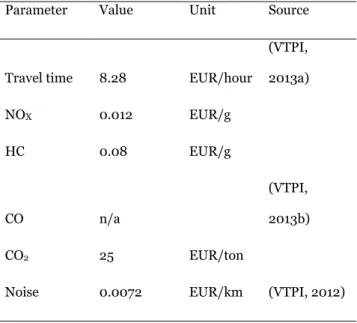
2.8. Weighing criteria and monetization of impacts

Different criteria and sources have been used to ponder the diverse analyzed parameters. Unless better local data are available, according to suggested in VTPI, (2013) work travel

time should be valued at wages and benefits, and that a default value for adult personal (including commuting) travel time should be 30% of household income per hour. Based on this methodology, for travel time costs the value 8.28€ per hour has been obtained.

Regarding noise effects literature tend to identify the marginal cost of additional vehicles on major highways and so are not sensitive to urban street traffic noise thus failing to consider for impacts, and incorporate arbitrary thresholds of traffic volumes and distance between homes and streets at which noise is considered a “problem.” For these reasons, such studies appear to undervalue urban traffic noise costs VTPI (2012). For monetize noise emissions costs we applied the methodology suggested in VTPI (2012) and we considered the value of 0.013 USD per mile which was estimated to be equivalent to 0.0072 EUR/km. Regarding air pollution emissions the monetization costs suggested by the Victoria Transport Policy Institute (VTPI, 2013b), which provides specific values for Portugal, were followed (see Table 1). Since the correlation between conflicts and accidents is not yet completed for the study area we did not consider an economic approach for this indicator.

Table 1 Considered Parameters cost factors

Parameter Value Unit Source

Travel time 8.28 EUR/hour

(VTPI, 2013a) NOX 0.012 EUR/g HC 0.08 EUR/g CO n/a (VTPI, 2013b) CO2 25 EUR/ton

Noise 0.0072 EUR/km (VTPI, 2012)

3. Results

This section presents and discusses and main the results of the previously described indicators. At the end a comprehensive and comparative analysis of the various analyzed parameters is performed.

3.1. Assessment of route choice impacts – individual perspective

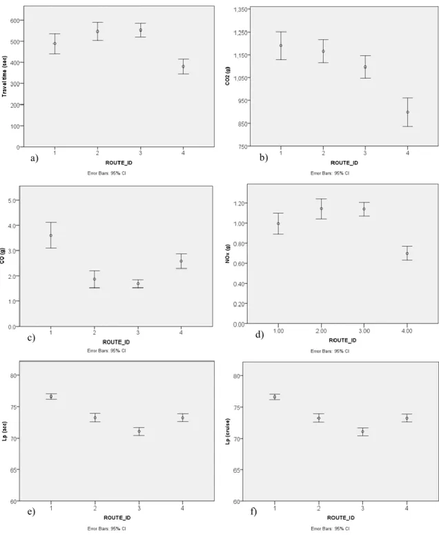
Fig. 6 shows the impact of different parameters according to route selection based on empirical data with error bars at 95%.

For the set of analyzed indicators, route 4 is the statistically significant best option regarding travel time (up 31% regarding the worst option), CO2 emissions and NOX

emissions (up to 13%). By contrast Route 3 is the best alternative as far as noise and CO emissions are concerned (up to 8 and 53%, respectively). This is explained due to the fact that this route is the shortest and virtually performed on urban routes with lower speeds. The impact due to the noise emission of a vehicle can be assessed monitoring the average

value of pressure level “immitted” at a certain distance, as described in section 2.4. These values represent the level that averagely occurs at 7.5 m during each route, both in the cruising/decelerating and in the accelerating states. Let us remind that Route 1 is mostly a motorway, Route 2 a national road, Route 3 an urban trip and Route 4 a mix of urban streets and national road. Route 3 presents the lower values of noise, due to the mainly urban trip and lower speeds. The higher values are obtained in Route 1, in which a motorway is present (higher speeds).

It can be noticed that the overall differences between cruising/decelerating and accelerating states are almost negligible. Only in Route 3, about 0,5 dBA difference occurs, probably due to the typology of roads during the trip. In urban trip, in fact, there is a higher number of stops or decelerations, because the existence of intersections with traffic lights roundabouts and stop controlled junctions and pedestrian crosswalks.

Fig. 6 Overall results for travel time and environmental indicators; a) Travel time; b) CO2; c)

CO; d) NOX; e)

Noise (at acceleration) and f) Noise (cruise)

a) b)

c) d)

Fig. 7 Left: Predicted number of conflicts for each route and, right: map of crash severity

Regarding safety, Fig 7 (left) shows the total number of conflicts (error bars at 95%) estimated from SSAM. For this parameter, it can be seen that routes 2 and 4 have a significant higher number of traffic conflicts mainly located at segment c which is a 2-lane national road with a relatively high demand (2400 vph). This section also includes an interchange with a motorway and finishes at a 3-lane roundabout which is a hotspot in terms of predicted conflicts, namely lane change and rear-end. Route 3 has a lower number of conflicts mainly because is the shortest route. Despite being the longest route, route 1 has a relatively low density of conflicts. Nevertheless as may be observed in the map (Fig 7 right), the severity of conflicts in the segment A of Route 1 (motorway) is noteworthy higher.

Table 2 summarizes the number and typology of conflicts.

Rout e TTC (s) PET (s) MaxS (m/s) DeltaS (s) DR (m/s) Total/per sim Rear End Lane Change Crossin g R1 1.090 1.590 7.957 4.869 -1.355 100.2 80.5 15.2 4.5 R2 0.901 1.012 10.161 7.076 -1.256 359.3 232.7 108.2 18.5 R3 1.079 1.439 7.334 4.230 -1.377 48.7 42.3 6.3 0.0 R4 0.935 1.176 8.208 5.964 -1.288 403.7 259.2 132.8 11.7

Legend: Time-to-collision (TTC); Post-encroachment time (PET); Maximum speed (MaxS);

Maximum speed differential (DeltaS); Deceleration rate (DR).

Note: The conflict type classification was made according to the Federal Highway Administration

criteria (Gettman et al., 2008)

Routes 2 and 4 present the lowest TTC and PET values, thus are the routes presenting the most severe conflicts. Route 2 presents Higher MaxS, and DeltaS, which means that there is a higher probability of severe potential collisions on that route. The findings for safety are not consensual. Route 3 presents less conflicts and these were less severe (lower TTC and PET). Also, this route yields the lower MaxS and DeltaS values which seem to suggest a low probability of severe potential collisions. However, DR (in absolute terms) is the highest computed value for all routes, maybe due to the high number of intersections. The results of Table 1 also confirm that routes 2 and 4 obtained the highest number of conflicts and these were more severe (low TTC and PET values). The evaluation report of SSAM model suggests the occurrence of conflicts and crashes may be to a certain extent distinct while still significantly related. The distribution of conflicts seems to lean more deeply toward “less harmful” conflicts events (i.e. rear ends) that do police-reported crash records. Therefore, the conflicts of different types (and corresponding severities) may exhibit different conflict-to-crash ratios. Taking into account the lack of information of severity and crash reports on the study area we will just use the total number of conflicts as a safety indicator. Moreover

from a driver perspective the existence of fewer decision points and traffic conflicts may simplify the driving task, increasing not only safety but also driving comfort.

3.2. Assessment of route choice impacts on other drivers (Indicators D and E).

Fig. 8 summarizes the marginal impact of the route of choice in rush hour taking into account the current demand values. Routes 1 and 3 are the routes where a higher marginal impact on all parameters is observed. This is due to the fact that these routes comprise segments with a observed higher Volume-to-Capacity (V/C) ratio where the tangent is steeper.

Routes 2 and 4 include sections on national highway whose incremental impact of demand is less noticeable. We also observed that CO2 and specially HC are the parameters

most affected by the increase in demand and consequent increase in travel time. CO emissions are rather less dependent on travel time and more affected by the acceleration system and high speeds. Obviously these results are only indicative of the general trend of the various routes to accommodate an increase in demand since in reality each individual driver exhibits a stochastic driver pattern. For instance, a vehicle can be more or less significantly affected in its performance by the time of arrival and time spent going through a corridor with traffic lights or roundabouts.

Fig. 8 Assessment of route choice impacts on route performance.

3.3 Assessment of route choice impacts on pedestrians, residents and workers (G and H)

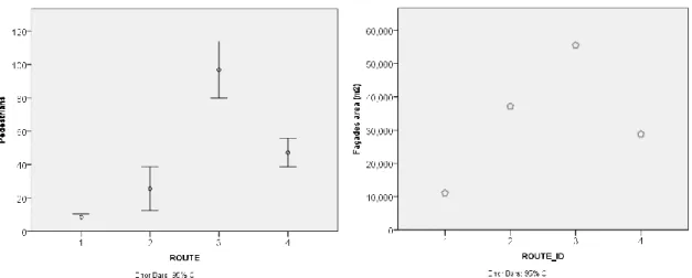
Fig. 9 illustrates the inductors F and G. F represents the average number of expected pedestrians (Fig. 9- left) walking in 9 sidewalks along both sides of a street for each route and potentially the ones more directly affected by traffic related externalities with local effect (e.g, noise, and CO emissions). Fig. 9 (right) shows the area of exposed façades for each route and must be seen as an additional indirect indicator of the number of citizen potentially exposed to local traffic-related effects. Route 3 exhibits the highest values both for the pedestrians and for the area of exposed façades. Route 1 which features a section on the motorway is by far the one with the lowest indicators of potential vulnerability to direct traffic effects. Route 2 and 4 shows an intermediate value in both indicators.

Fig. 9 Left: Expected number of affected pedestrians and, Right: exposed façades area.

Table 3 Overall results for the analysed indicators Indicator Unit Route 1 Route 2 Route 3 Route 4 Route 1 Route 2 Route 3 Route 4 A0 Distance (m) 6010 5900 3900 4117 1.00 0.98 0.65 0.69 A1 Travel time costs (EUR) 1.12 1.26 1.27 0.87 0.88 0.99 1.00 0.69

A2 Fuel Use costs (lEUR 0.71 0.69 0.65 0.54 1.00 0.98 0.92 0.76

A Travel costs (EUR ) 1.83 1.95 1.92 1.41 0.94 1.00 0.99 0.72 A3 Conflicts numbe r 100 359 49 404 0.25 0.89 0.12 1.00 B1 CO (g) 3.61 1.87 1.68 2.58 1.00 0.52 0.47 0.72 B2 NOX (g) 0.99 1.142 1.139 0.99 0.87 1.00 1.00 0.87 B3 HC (g) 0.13 0.13 0.10 0.97 1.00 0.95 0.72 C1 CO2 (g) 1190 1166 1096 898 1.00 0.98 0.92 0.76 B4 Noise (db) 76.53 73.12 70.69 73.16 1.00 0.96 0.92 0.96 B Local Env. costs (EUR) 0.022 0.024 0.023 0.019 0.91 1.00 0.98 0.81 C Global Env. Costs (EUR) 0.030 0.029 0.027 0.022 1.00 0.98 0.92 0.76 C+

B Total Env. Costs (EUR) 0.051 0.053 0.051 0.042 0.97 1.00 0.96 0.79

D1 CO (%) 0.26 0.22 0.40 0.20 0.65 0.54 1.00 0.51 D2 NOX (%) 0.31 0.21 0.54 0.23 0.58 0.40 1.00 0.43 D3 HC (%) 0.93 0.38 1.07 0.51 0.87 0.35 1.00 0.48 E1 CO2 (%) 0.34 0.21 0.56 0.24 0.61 0.37 1.00 0.43 F1 Travel time (%) 0.72 0.20 0.69 0.37 1.00 0.28 0.96 0.52 G Pedestrians numbe r 9.60 25.60 96.80 47.20 0.10 0.26 1.00 0.49 H Exposed Façade (ha) 1.11 3.71 5.55 2.88 0.20 0.67 1.00 0.52

Table 3 quantifies the overall results presented previously for each route and provides economic cost values based on the monetization criteria presented in 2.8. For facilitating a

comparative analysis among indicators, the four right columns show the relative results represented by a graduation of colors on the various parameters analyzed (darker cells are worse options for each indicator).

The indicators "A" represent the individual and direct impacts for drivers. Clearly, route 4 performs better in terms of driver’s costs. Albeit short, Route 3 is strongly penalized by its substantially higher travel time. At the same time, this route is the safest option in terms of conflicts occurrence. Route 4 shows a higher probability of occurrence of conflicts resulting in a trade-off between the minimization of conflicts/safety and drivers costs.

Regarding environmental parameters, even though Route 3 enables greater savings in CO and noise emissions, route 4 is generally the itinerary that enables the minimization of environmental costs. Thus, an eco-routing algorithm based on absolute minimization of emissions would suggest Route 4 as the best option. In this case (for this type of vehicle and OD pair) and from the point of view of personal and environmental costs, the options are coincident which enhancing the viability of eco-friendly choice options by drivers.

The picture becomes more complex when other parts are taken into account. With regard to the impact on other drivers (indicators D and E), route 2 is the option enabling a lower marginal impact on both the travel time and emissions, while routes 1 and 3 show higher marginal impacts on other drivers performance. While for a single vehicle the absolute values per vehicle may be considered negligible, these indicators based on link-performance functions would certainly be a factor to consider when assigning subpopulation/platoons of vehicles in a context of a centralized/automated traffic management center.

Regarding the exposed population, here represented by pedestrians and other citizens living/working in buildings within 50 m from each route, a clear trade-off between the minimization of impacts, personal costs and the minimization of exposed population can be identified. In this case, route 1 is by far the alternative that minimizes the number of citizens

potentially exposed to traffic impacts. However, it is also the option that leads to a higher amount of emissions generated by vehicles.

Figure 10 exemplifies how some of the main indicators obtained can be reflected in the triangular diagram of sustainability (see Fig. 1). The pillar "environment" is represented by the full environmental costs (C + B). The pillar "economy" here is focused in the individual costs of travel along each route (A). The social pillar is only indicative and is represented by the mean of G and H indicators. The social aspect is the most critical and its final

dimension must be estimated after estimating the actual levels of population exposure to traffic-related effects.

For each dimension of sustainability, the route with the best indicator has the circle with maximum radius (100%) centered in the respective triangle vertex. The remaining routes have a circle with a radius proportional to the value obtained for that dimension. In the diagrams of Fig. 10, the circles overlap iff at least two circles present a radius greater than 2/3 of the largest diameter circle for the set of analysed routes.

The interaction between environmental and economic areas shows to what extent it would be viable to ask drivers to choose an environmentally friendly route. The interaction between the economic and social dimension provide insights into equitability issues namely the distribution of efforts, costs and impacts among drivers and non-road users. The intersection of the environmental and social dimensions leads to the consideration of the bearable environment. Namely it shows the relationship between the absolute amount of generated environmental impacts and the impacts potentially felt by local communities. Figure 10 suggest that that although route 4 present the best results in the economic and environmental fields, only in Route 1 all domains can be overlapped suggesting that this is unique viable, bearable and equitable salutation. In fact, from the point of view of urban sustainability it seems logical to divert traffic from city centers for city rings. However, this option has the following problems:

a) We would be giving privileging to routes whose local impacts would be smaller but simultaneously we would be promoting an increase in CO2 emissions in the atmosphere with

impacts on a global scale (similar problem identified by Kickhöfer and Kern (2015);

b) From the methodological point of view, such approach lack of scientific basis in several aspects: i) the actual exposure (concentration*time) of the population to noise and air pollutants is not yet known, ii) the monetization costs used in the study should be adapted to characterize with a higher degree of resolution local contexts; iii) special emphasis should be given to the most vulnerable population (such as elderly and children).

4. Conclusions and Future work

In this work empirical GPS data, microscopic simulation models of traffic, pollutant emissions and noise, as well as a road conflict prediction platform, were used to characterize in detail 4 routes of a origin/destination pair. In addition to the traditional indicators taken

into account in common navigation systems and even in eco-routing systems, new variables have been considered such as noise and road safety. A novelty was also the preliminary inclusion of social criteria in defining sustainable routes.

In addition to some trade-offs identified in the field of absolute minimization of environmental indicators (e.g. CO and Noise vs. other pollutants), the most obvious conflict was between the minimization of environmental costs and the exposed population to local traffic externalities. In particular, the route that minimizes pollutant emissions presents 4 times more pedestrians subject to traffic impacts and the route with the lowest mean noise value has 9 times more pedestrians that the route with fewer number of pedestrians. In summary if we consider the ratio between the maximum relative difference for each indicator, travel individual costs varies up to a ratio of 1.39; the probability of conflicts can vary by a factor of 4, pollutant emissions generated vary up to 1.39, and noise up to 1.08. If we consider the impacts on other drivers and non-road users we may observe a relative variation in the impact caused to other drivers of 3.5 and the number of potential people affected traffic local impacts by a factor of 10 times.

The present work should be seen as a first approach to identify conflicts of interest in the field of sustainable traffic assignment and cooperative road management. An evident conclusion is that the range of variation of the potential of affected people may be much higher than that the estimated relative differences in the amount of total pollution among all routes. This fact highlights the need to take into account the urban activity patterns if we want to provide quality information on environmentally friendly routes beyond the CO2

factor. In the context of implementation of real-time traffic management systems, the findings suggest the need for the inclusion of automatic systems for activity monitoring namely the spatiotemporal distribution of population in cities. Future research should explore the application of supplementary data sources to develop temporally sensitive models involving the daytime distribution of various vulnerable groups. In addition to

commuting and employment, information on people in daytime institutions (e.g., schools / hospitals), remote sensing, radiofrequency and activity-space analysis technologies can be used to calibrate and develop an independent model of the urban people distribution. In order to better determine population exposure to pollution, several air quality scenarios may be assessed based on mesoscale and statistical dispersion models (e.g. an artificial neural network model), which could allow the development of a spatiotemporal database of air pollutant concentrations and the identification of critical pollution hotspots as a function of different congestion scenarios and weather conditions. This analysis will be an important input for implementing an online cooperative traffic management system (an on-going project of the research team).

Acknowledgements

The authors acknowledge the support of the Portuguese Science and Technology

Foundation - FCT for the grants SFRH/BPD/100703/2014 and SFRH/BD/87402/2012, as well as the R&D project PTDC/EMS-TRA/0383/2014. The authors acknowledge Toyota Caetano Portugal.

References

ACAP, 2012. Automotive Industry Statistics 2010 Edition.

Ahn, K., Rakha, H. a., 2013. Network-wide impacts of eco-routing strategies: A large-scale case study. Transportation Research Part D: Transport and Environment 25, 119–130.

Ahn, K.G., Rakha, H., 2008. The effects of route choice decisions on vehicle energy consumption and emissions. Transportation Research Part D-Transport and Environment 13, 151–167.

Bandeira, J.M., Carvalho, D., Khattak, A., Rouphail, N., Fontes, T., Fernandes, P., M.C., C., n.d. Empirical assessment of route choice impact on emissions over different congestion scenarios. International Journal of Sustainable Transportation.

Bandeira, J.M, Pereira, S.F., Fontes, T., Fernandes, P., Khattak, A.J., Coelho, M.C., 2014. Assessing the importance of vehicle type for the implementation of eco-routing systems. Transport Research Procedia 00, 2–4.

Bandeira, J.M., Almeida, T.G., Khattak, A.J., Rouphail, N.M., Coelho, M.C., 2013. Generating Emissions Information for Route Selection: Experimental Monitoring and Routes Characterization. Journal of Intelligent Transportation Systems 17, 3–17.

Barth, M., Boriboonsomsin, K., Vu, A., 2007. Environmentally-Friendly Navigation. In: Proceedings of the 2007 IEEE Intelligent Transportation Systems Conference.

Beelen, R., Hoek, G., van den Brandt, P. a., Goldbohm, R.A., Fischer, P., Schouten, L.J., Jerrett, M., Hughes, E., Armstrong, B., Brunekreef, B., 2007. Long-Term Effects of Traffic-Related Air Pollution on Mortality in a Dutch Cohort (NLCS-AIR Study). Environmental Health Perspectives 116, 196–202.

Boriboonsomsin, K., Joseph, D., Barth, M., 2014. An Examination of the Attributes and Value of Eco - Friendly Route Choices. Transportation Research Record, Journal of the Transportation Research Board 20427, 13– 25.

Bühlmann, E., Sandberg, U., Mioduszewski, P., n.d. Speed dependency of temperature effects on road traffic noise. Internoise 2015.

CMA, 2015. City of Aveiro [WWW Document]. URL www.cm-aveiro.pt

Coelho, M.C., Fontes, T., Bandeira, J.M., Pereira, S.R., Tchepel, O., Dias, D., Sá, E., Amorim, J.H., Borrego, C., 2013. Assessment of potential improvements on regional air quality modelling related with implementation of a detailed methodology for traffic emission estimation. The Science of the total environment 470-471C, 127–137.

Coelho, M.C., Frey, H.C., Rouphail, N.M., Zhai, H., Pelkmans, L., 2009. Assessing methods for comparing emissions from gasoline and diesel light-duty vehicles based on microscale measurements. Transportation Research Part D-Transport and Environment 14, 91–99.

European Commission, n.d. Roadmap to a Single European Transport Area - Transport Matters [WWW Document]. URL

http://ec.europa.eu/transport/strategies/facts-and-figures/transport-matters/index_en.htm

European Commission - EC, 2011. EG FTF - 1st Report of the Expert Group: Future Transport Fuels. European Environmental Agency - EEA, 2013. European Environment Agency. EMEP/EEA air pollutant

Ferguson, E.M., Duthie, J., Travis Waller, S., 2012. Comparing Delay Minimization and Emissions

Minimization in the Network Design Problem. Computer-Aided Civil and Infrastructure Engineering 27, 288–302.

Finkelstein, M.M., Jerrett, M., Sears, M.R., 2004. Traffic Air Pollution and Mortality Rate Advancement Periods. American Journal of Epidemiology 160, 173–177.

Folberth, G.A., Hauglustaine, D.A., Lathière, J., Brocheton, F., 2006. Interactive chemistry in the Laboratoire de Météorologie Dynamique general circulation model: model description and impact analysis of biogenic hydrocarbons on tropospheric chemistry. Atmos. Chem. Phys. 6, 2273–2319.

Fontes, T., Fernandes, P., Rodrigues, H., Bandeira, J.M., Pereira, S.R., Khattak, A.J., Coelho, M.C., 2014. Are HOV/eco-lanes a sustainable option to reducing emissions in a medium-sized European city?

Transportation Research Part A: Policy and Practice 63, 93–106.

Frey, H.C., Zhang, K.S., Rouphail, N.M., 2008. Fuel use and emissions comparisons for alternative routes, time of day, road grade, and vehicles based on in-use measurements. Environmental Science & Technology 42, 2483–2489.

Garg, N., Maji, S., 2014. A critical review of principal traffic noise models: Strategies and implications. Environmental Impact Assessment Review 46, 68–81.

Gettman, D., Pu, L., Sayed, T., G., S.S., 2008. Surrogate safety assessment model and 1 validation: final report. FHWA-HRT-08-051, FHWA, 2008.

Guarnaccia C ., Nikos E. Mastorakis and Joseph Quartieri, T.L.L.L., 2011. A Comparison between Traffic Noise Experimental Data and Predictive Models Results. International Journal of Mechanics 5, 379–386. Guarnaccia, C., 2013. Advanced Tools for Traffic Noise Modelling and Prediction noise. WSEAS

TRANSACTIONS on SYSTEMS 12, 121–130.

Guo, L., Huang, S., Sadek, A.W., 2013. An Evaluation of Environmental Benefits of Time-Dependent Green Routing in the Greater Buffalo–Niagara Region. Journal of Intelligent Transportation Systems 17, 18–30. Gwo-Hshiung, T., Chien-Ho, C., 1993. Multiobjective decision making for traffic assignment. IEEE

Transactions on Engineering Management 40, 180–187.

Hale, D., 1997. “How Many Netsim Runs Are Enough?” McTrans 11, 1–9.

HEI, 2010. Traffic-related air pollution: a critical review of the literature on emissions, exposure, and health effects Special Report, Health Effects Institute.

Hoek, G., Brunekreef, B., Goldbohm, S., Fischer, P., Van Den Brandt, P. a., 2002. Association between mortality and indicators of traffic-related air pollution in the Netherlands: A cohort study. Lancet 360, 1203–1209.

Hughes, B.P., Newstead, S., Anund, a., Shu, C.C., Falkmer, T., 2015. A review of models relevant to road safety. Accident Analysis & Prevention 74, 250–270.

Iannone, G., Guarnaccia, C., Quartieri, J., 2013. Speed Distribution Influence in Road Traffic Noise Prediction 12, 493–501.

Kephalopoulos, Stylianos Paviotti, M., Anfosso-Lédée, F., 2012. Common Noise Assessment Methods in Europe (CNOSSOS‐EU).

Kickhöfer, B., Kern, J., 2015. Pricing local emission exposure of road traffic: An agent-based approach. Transportation Research Part D: Transport and Environment 37, 14–28.

Lelong, J., 1999. Vehicle noise emission: evaluation of tyre/road-and motornoise contributions,. In: Proceedings of Internoise 99 – The 1999 International Congress on Noise Control Engineering. Fort Lauderdale, pp. 203–208.

Levin, M.W., Jafari, E., Shah, R., Ruiz-Juri, N., Mouskos, K.C., 2014. A Dynamic Traffic Assignment

Framework to Assess the Short-Term Network-Level Impacts of Eco-Routing Strategies. TRB 93rd Annual Meeting Compendium of Papers.

Minett, C., Arem, B. van, Kuijpers, S., 2011. Eco-routing: comparing the fuel consumption of different routes between an origin and destination using field test speed profiles and synthetic speed profiles. In: IEEE Forum on Integrated and Sustainable Transportation Systems June 29 - July 1, 2011. Vienna.

NoiseInEU, 2015. No!se in EU [WWW Document]. OCDE, 2014. The Cost of Air Pollution. OCDE Publishing.

Peeters, B., 2007. The noise emission model for European road traffic.

Pereira, S.R., Fontes, T., Bandeira, J.M., Fernandes, P., M.C., C., 2014. SmartDecision: A Route Choice App Based on Eco-Friendly Criteria. In: TRB 94th Annual Meeting Compendium of Papers.

PTV, 2005. VISSIM 410 Users’ Manual.

Shilton, S.J., Ledee, F.A., Leeuwen, H. van, 2015. Conversion of existing road source data to use. In: Proceedings of the 2015 Euronoise Conference.

Smit, R., Brown, a. L., Chan, Y.C., 2008. Do air pollution emissions and fuel consumption models for roadways include the effects of congestion in the roadway traffic flow? Environmental Modelling & Software 23, 1262–1270.

UN, 2014. World Urbanization Prospects - The 2014 Revision, ST/ESA/SER.A/352. New York, US. United Nations, 2014. United Nations Environment Programme [WWW Document]. URL

http://www.unep.org/urban_environment/issues/urban_air.asp VTPI, 2012. Transportation Cost and Benefit Analysis II – Noise Costs 1–16.

VTPI, 2013a. Transportation Cost and Benefit Analysis II – Travel Time Costs.

VTPI, 2013b. Transportation Cost and Benefit Analysis II – Air Pollution Costs. Transportation Cost and Benefit Analysis 1–33.

Wismans, L., Van Berkum, E., Bliemer, M., 2011. Modelling Externalities using Dynamic Traffic Assignment Models: A Review. Transport Reviews 31, 521–545.

Zhang, Y.L., Lv, J.P., Ying, Q., 2010. Traffic assignment considering air quality. Transportation Research Part D-Transport and Environment 15, 497–502.