Finding simple strategies for high returns

(1)

Master Thesis Finding Simple Strategies for High Returns

Dissertation (Value & Momentum)

Finding Simple Strategies for High Returns

Value & Momentum

Francisco Pinto Coelho

Dissertation written under the supervision of Professor Franck Bancel

Dissertation submitted in partial fulfilment of requirements for the MSc in Double Degree Program, at Católica Lisbon School of Business & Economics, May 6th

(2)

1

Keywords: Value, Momentum, Earnings Momentum, Acceleration, Investment Strategies; Empirical Finance

Abstract

My objective throughout this paper is to provide useful insights to investors on simple ways to obtain high return focusing on Value & Momentum strategies applied to the US Market. Opposite from most existing literature, we were not able to prove the existence of both Price and Earnings Momentum. However, we see that past returns are explanatory of future for the same stock, as predicted by Moskowitz, Ooi and Pederson (2012). We observe that Value yield positive and abnormal returns, confirming past literature. Nonetheless, both strategies seem to be underperforming as they are not able to efficiently distinguish between true and false winners and losers. In order to solve this problem, I double sorted Value & Momentum using financial ratios and short-term trend indicators (acceleration indexes). For Momentum, generally, double sorting was either slightly or ineffective at all. For Value, double sorting improved returns suggesting that Price Earnings and Price to Cash-flow add complementary information to each other. After Accelerating Value & Momentum, we were able to establish the most profitable returns. However, the best possible risk-adjusted solution is the one proposed by Asness, Moskowitz & Pedersen (2013): an equal-weighted combination of returns.

(3)

2 Palavras-chave: Value, Momentum, Earnings Momentum, Aceleração, Estratégias de Investimento; Empirical Finance

Abstract

O objetivo principal deste paper é providenciar formas simples de obter retornos elevados focando em estratégias Value & Momentum aplicadas ao mercado Americano. Contrario à literatura existente, não pudemos provar a existência de Price e Earnings Momentum. Contudo, observamos que para a mesma Ação (Stock), retornos passados são indicadores relevantes de retornos futuros, tal como mencionado por Moskowitz, Ooi and Pederson (2012). Para além disso, podemos verificar que estratégias Value providenciam retornos anormais e positivos, confirmando os resultados de literatura existente. No entanto, ambas as estratégias Value e Momentum apresentam resultados aquém do esperado, uma vez que não são significativamente capazes de distinguir entre os verdadeiros e falsos winners e losers. De modo a resolver este problema, Value e Momentum foram filtrados duplamente utilizando rácios financeiros e indicadores de tendência de curto prazo (Índices de Aceleração). Momentum filtrado duas vezes por rácios financeiros, foi geralmente ineficiente. Por outro lado, para Value, pudemos observar que a dupla filtragem melhorou os resultados gerais, sugerindo que os rácios Price-Earnings e Cash-Flow to Price adicionam informação complementar um ao outro. Depois de acelerar Value e Momentum, fomos capazes de observar as estratégias com maior retorno. Contudo, a melhor solução ajustada ao risco é a mesma sugerida por Asness, Moskowitz & Pedersen (2013): uma combinação com pesos iguais de Value e Momentum, embora neste caso acelerados.

(4)

(5)

4

Table of Contents

Introduction & Methodology ... 1

Literature Review ... 3

A. Momentum Strategies ... 3

B. Value ... 7

C. Final Remarks... 9

I. Data & Methodology ... 10

I.I The Sample ... 10

I.II Price Momentum ... 11

I.II.I Acceleration Index ... 12

I.III Earnings Momentum & Value ... 12

I.IV Performance Measures ... 13

II. Empirical Results ... 14

II.I Price Momentum Analysis ... 14

I.I.I Momentum sorted by fundamental ratios ... 15

II.I.II Accelerated Momentum ... 22

II.II Earnings Momentum ... 25

II.II.I Double Sorted Earnings Momentum ... 28

II.II.II Accelerated Earnings Momentum ... 29

II.III Value Analysis ... 33

II.III.I Double Sorted Value ... 37

II.III.II Accelerated Value... 40

III.Overall Best ... 43

I. Drawbacks & Conclusions ... 45

III.I Model Drawbacks ... 45

III.II Concluding Remarks ... 45

III.II.I Momentum ... 46

III.II.II Value ... 48

APPENDIX ... 49

(6)

1

Introduction & Methodology

Ever since its creation, stock markets have been having a growing importance on the economy. Many authors like Nelson (1976), Bodie (1976), Fama & Schwert (1977) claimed the existence of a negative correlation between stock returns and inflation, which is claimed by Fama (1981) to be negatively correlated to real activity1. The latter mentioned author also

states the existence of a positive relation between stock returns and some other real variables: capital expenditure, real rate of return on capital and output (Fama (1981)) or even industrial production as proved by Domian & Louton (1997). Furthermore, according to Levine & Zervos (1998), stock market liquidity is a “robust predictor of real per capita gross domestic product (GDP) growth for more than 40 countries.

Sharpe (1964) and Lintner’s (1965) Capital Asset Pricing Model (CAPM) marks the birth of asset pricing theory (Fama & French, 2004). According to the CAPM, the expected excess return of every security is proportional to its systematic risk (beta) with respect to the market portfolio. However, since shortly after it was published, research showed that the model empirically fails. Friend and Blume (1970) concluded that CAPM consistently overestimates the cost of equity for high beta stocks and underestimates for low ones. Also, other variables than Beta are proven to be positively correlated to stock returns, meaning that systematic risk is not the only factor useful to predict returns. Other ones have been proved valuable: Market Capitalization (Banz (1981)), leverage (Bhandari (1988)) and book-to-market ratio (Rosenberg et al. (1985), Chan, Hamao, and Lakonishok (1991)). Fama & French (1992) also mention that companies’ size, book-to-market ratio, Earnings-Price or Dividend-price have a strong explanatory power over stock returns, while being low correlated to each other.

Most of these studies can be separated into two categories: Value & Momentum. Value strategies are supported by the fact that firms with low price-to-financials (Market to book, Price to Equity, Price to Cash-flow, …) are overvalued. Momentum strategies show that past stock performance is correlated to the futures’.

In fact, once we categorize these empirical studies one can realize that Momentum and value effects are some of the most studied capital market phenomena and yet still yielding positive abnormal returns. One of the most recent authors, Asness, Moskowitz & Pedersen (2013)

(7)

2 showed that these methodologies are useful tools to predict returns on a global scale (U.S., U.K., Continental Europe and Japan and across different asset classes (individual stocks, equity index futures, government bonds, currencies and commodity futures). Bird, Ron and Whitaker (2004) also confirmed the predictive power of both strategies combined in major European markets, whereas Zhang, Brown, Yan Du and Rhee (2008) were not able to demonstrate Value effects in Asian markets.

Most times, Value and Momentum are studied separately and out of context. Therefore, the aim of this project is to extend and unify the analysis of phenomena, exposing connections between them and identifying the power of their combination to predict future stock performance. In order to keep a commonly known reference point, throughout this analysis results will be compared to the market returns.

(8)

3

Literature Review

A. Momentum Strategies

Momentum strategies are defined by Asness, Moskowitz & Pedersen (2013) as the “relationship between an asset’s return and its recent relative performance in history”.

Poterba & Summers (1988) and Fama & French (1988) prove that stock prices follow a mean reverting process in US markets, i.e. that there is a tendency for the price to return to its trend. Richards (1997), Balvers, Wu & Gilliland (2000) also prove this theory for international equity indexes. Therefore, it seems reasonable and intuitive to assume that if stocks provide high mid-term past performance, they will continue to do it in the future. However, Lo & Mckinlay (1988), Kim et. al (1991) argue that this phenomenon is not verified or only under certain conditions, respectively. Inclusively, Horne & Parker (1967) and Fama (1995) prove that stocks price variations are mostly independent from each other, meaning that they are not significantly predictable. The fact that Momentum’s base assumptions do not seem to be clearly proved constitutes an argument in favor of studying this phenomenon.

Bird & Whitaker (2003) establish two different types of Momentum based on the different sources used to track relative performance and establish portfolio weights. Price Momentum theory states that historical stock market prices are a proxy for future returns while Earnings Momentum assumes that information provided by financial reports and/or analysts’ forecasts can explain future returns on equity investments. Moskowitz, Ooi & Pedersen (2012) also mention a third form of Momentum based on each stock’s time series instead focusing on the cross-sectional relative returns (Price and Earnings Momentum). They verified that across different markets and asset classes, each instrument’s 12-month excess returns are positive predictors of its own future returns.

The history of the Price Momentum anomaly dates from 1993 with Jegadeesh & Titman (1993) who first proved that buying stocks with high returns and selling those with low ones yield positive and statistically significant results. Chan, Jegadeesh & Lakonishok (1996), Haugen & Baker (1996), Bird & Casavecchia (2007), Asness, Moskowitz & Pedersen (2013), among others, attested this phenomenon across different countries and asset classes such as U.S., U.K., Continental Europe and Japan, individual stocks, equity index futures, government bonds, currencies and commodity futures. Rouwenhorst (1998) also proves Price Momentum among 20 emerging market. However, others like Zhang et al (2008) were not

(9)

4 able to find the evidence of such effect in Asian markets. Some other authors also proved the success of Price Momentum under different circumstances: Bernard & Thomas (1989,1990) conclude that this type of investment strategy yield positive and significant abnormal returns even after controlling for post-earnings-announcement drift. The explanation of this phenomenon is still controversial. However, Conrad and Kaul (1998), Chordia and Shivakumar, (2002) state that it represents a compensation for the implicit increase in systematic risk when comparing to other strategies. De Long et al (1990) conclude that Price Momentum returns can be driven by investors’ overreaction given the success of a certain asset. In another words, “trend-chasers” reinforce price movements, explaining the abnormal returns. Vayanos & Woolley (2013) by creating a model where Momentum depends on delegated management, shows that slow capital movement between investment funds can drive prices further from fundamentals causing future price reversals, explaining both value and Momentum. Thus, I expect that after applying this strategy, stocks with the highest (lowest) past returns, i.e. Momentum winners (losers), yield positive (negative) and significant future outcomes. This will lead to even better outcomes if we consider longing the winners and shorting the losers (spread portfolio).

Bird & Casavecchia (2007) claimed that Price Momentum returns can be enhanced using acceleration indexes. Not applying those can result into misleading conclusions as stocks with a positive or negative Momentum can have an upward, stabilizing or downward price trend. In another words, sole Momentum lacks the ability to sort between three types of stocks, according to the same authors: the first ones (Type One) are those which start performing soon after they were identified as winners) or losers, i.e., with high or low Value & Momentum, respectively. The second type (Type Two) includes stocks which only start suffering from a significant price variation towards a trend (up or downwards) in a mid-term range. The last ones (Type Three) are those which do never outperform (stable price returns) or have a price trend towards a different direction than the expected.

Distinguishing between these three types of assets will allow a better identification of both winners and losers (Type One), leading to potential higher spread portfolios – higher return for winners and lower for losers.

In order to solve this problem, we will try two different approaches: the first, using the acceleration indexes provided by Bird & Casavecchia (2007). Those are ratios between different time span Momentums, which allow determining the slope of the cumulated returns. I expect that after applied to Value & Momentum, high slopes (acceleration) imply higher

(10)

5 returns, then each of the phenomena on a stand-alone basis. On the other hand, low slopes should require lower returns than Value & Momentum alone.

Secondly, each Price Momentum portfolio will be sorted into others based on firm’s financial ratios (Earnings Momentum). This will enable us to conclude whether past fundamental financial ratios2, add or not any relevant information to the one absorbed by the market prices.

It can also happen that Price Momentum's overall performance is negatively affected by Earnings Momentum. While ratios are released on a general basis within each three months, market prices are updated constantly with expectations and recent news3 that can have a

lagged impact on the company's financials. For that reason, one can expect Price Momentum’s ability to explain future returns to decrease after double sorting by financial ratios. On the other hand, financial analysts are widely known amongst literature to overreact to information (De Bondt & Thaler (1985, 1987), Easterwood & Nutt (1998), Chopra, Lakonishok & Ritter (1992), Abarbanell & Bernard (1992), Lim (2001), …). As key financials represent pure firm conditions with low level of subjective opinions, from which stock prices calculations are derived, one can argue that firms that hold financially well in the present will perform well in the future. Concluding, accelerating and double sorting Momentum are my two hypotheses to distinguish Type One assets from the remaining and consequently obtain better results using a spread portfolio.

Several authors proved the existence of abnormal returns yielded by Earnings Momentum; According to Mao & Wei (2014), Ball & Brown (1968) were the first ones to mention this effect. However, there is a divergence on the methodology used. Most of them, such as Chan, Jegadeesh & Lakonishok (1996), Bird & Whitaker (2003), Mao & Wei (2014), among others estimate Earnings Momentum based on earnings’ positive or negative surprise versus analyst consensus expectations. Using this approach, Griffin, Ji & Spencer (2003) proved the existence of earnings Momentum strategies across north and south American markets, most of European countries, some and Asian. Schneider & Gaunt (2012) stated the same conclusion for Australian equity markets.

Chan, Jegadeesh & Lakonishok (1996) claim that a possible explanation for Earnings Momentum approach’s abnormal returns is the fact that it takes advantage of stock price delayed reactions to certain events. In other words, for good (bad) news, financials are already

2 Financial ratios and its respective analysis reason of application is explained below on Earnings Momentum 3 Note that we call news to any extra-ordinary event that may occur during the financial year that is publicly

(11)

6 high (lower) but stock prices are still lower (higher) than they should. Assuming market efficiency, stock prices will soon adjust to its fair value, driving undervalued prices to go up (winners) and overvalued to go down (losers) and consequently Earnings Momentum to yield a positive outcome. However, for this theory to be verified, one should expect a high correlation between Earnings and Price Momentum strategies, since Momentum exists due to stock prices’ adaption to firms’ financial reality.

On the other hand, the opposite situation can also happen: if market prices react immediately to released information and financial ratios do not, its explanatory power of future returns will decrease and Earnings Momentum will not likely yield positive and significant returns. In fact, Khotari & Warner (2005) claim that more than 500 papers have been published in top financial journals stating that stock prices significantly react to news. This means that financial ratios might not fully reflect future company reality as market prices. Therefore, adding market information to financial ratios is one of the reasons why Earnings Momentum will also be sorted by acceleration indexes. Also, even if Earnings Momentum portfolios are able to select stocks with future growth and decline, they fail to identify when it will happen. Similar to Price Momentum, exclusively based on Earnings Momentum it is difficult to distinguish between Type One, Two or Three assets. Therefore, acceleration might prove as useful as it is expected to Price Momentum: it is expected to enhance both winners’ growing and losers’ declining price trends, creating spread portfolios with even higher returns.

Despite occurring earlier in time and being updated more frequently than reported earnings, analysts’ forecasts will not be used during the current study for two major reasons: (1) for some firms data is hard to obtain for a sample large enough to represent the analysts’ consensus on a given price and (2) because one of this study’s objectives is to conclude whether past/present information is better predictor of future stock prices than forward-looking one, such as an asset’s market prices or analyst’s forecasts. This changes a little the base hypotheses of Earnings Momentum. Instead of believing that firms with higher analyst recommendations or most number of earnings surprise outperform, we will try to prove if firms with highest (lowest) financial returns provide is the greatest and positive (lowest and negative) the future price returns.

Myers, Myers & Skinner (2007), followed our desired approach, proving that firms who present high levels of Earnings per Share (EPS) not only keep the trend on the forthcoming years but also show “abnormally strong market performances” during the same period. During

(12)

7 the current work, I will extend the previous author’s methodology to other ratios, since I believe that one single indicator is not representative of the whole firm’s condition. Thus, it is expected that sorting portfolios based on a combination of different financial ratios will yield better returns than each one solely, as I believe them to have complementary information. In my opinion, there are four critical areas which can affect a company’s performance: Profitability (Earnings per Share - EPS), Liquidity (Current Ratio – current assets/current liabilities), Risk (Debt-to-equity – D/E) and Efficiency (Asset Turnover – Sales/Total Assets). The reason why we use ratios instead of sole financials (sales, earnings, assets or debt) is to control for size, as it might be argued that bigger companies provide higher financials but not necessary greater ratios and stock price returns. Fama & French (1995, 2012), for example, proved that smaller firms provide higher outcomes, stressing our need to control for this variable.

As mentioned before, my hypothesis is that firms with higher profitability, liquidity, risk or efficiency will yield positive and significant returns and firms which have a greater combination of those measurements will yield even higher. On the contrary, firms with the lowest levels of those measurements will provide negative and significant outcomes, leading to higher spread portfolios.

B. Value

According to Bird & Whitaker (2003), Value based strategies include investing on undervalued stocks (Value stocks) and selling those which are overly expensive, also called growth or glamour stocks. Previous authors such as Fama & French (1992, 2012), Lakonishok, Shleifer & Vishny (1994), Bird & Whitaker (2003), Bird & Casavecchia (2007), Asness, Moskowitz & Pedersen (2013), among others proved that on average higher returns are yielded by stocks with low levels of some price to fundamental value ratios such as: Price Earnings (P/E - Basu (1977), Jaffe, Keim, and Westerfield (1989), Chan, Hamao, and Lakonishok (1991), and Fama and French (1992)), book-to-market value of equity (B/M - Rosenberg, Reid, and Lanstein (1984), Asness, Moskowitz & Pedersen (2013), Fama & French (2012)) or price to Cash flow (P/CF - Chan, Hamao, and Lakonishok (1991)).

Asness, Moskowitz & Pedersen (2013) and Fama & French (2012) and other authors proved the existence of Value based strategies across international markets (U.S., U.K., Europe and

(13)

8 Asia Pacific4), through different industries (Moskowitz & Grinblatt (1999)) and asset classes,

such as: government bonds (Asness, Moskowitz & Pedersen (2013)), currencies (Asness, Moskowitz & Pedersen (2013)), commodities (Erb & Harvey (2006)) and even international bond futures (Asness, Moskowitz & Pedersen (2013)).

The explanation why Value strategies yield abnormal returns still remains on controversial. However, most authors explained using behavioral arguments. Lakonishok, Shleifer & Vishny (1994) claim that investors tend to get “overly excited” regarding stocks with past high performance. This over-investment leads to a price inflation not reflected on the fundamentals to price ratio (glamour stocks). The same happens to assets with decreasing past returns, with which investors get “overly concerned”, leading to an overall decrease in the investment and price to deflate (value stocks). As value strategies invest on low price to fundamentals, the counter-cycle investment leads to abnormal returns. Fama & French (1992) claim that value strategies bear high fundamental risk. Therefore proven abnormal returns are a compensation for bearing this risk.

Past literature focuses on one indicator to explain stocks’ excess returns, either on PE, BM or P/CF. However, one can say that different indicators provide complementary information regarding a given firm. For example, Barbee, Mukherji & Rains (1996) proved that between 1971 to 1991 Sales to Price had a higher explanatory power over stock returns than Book-to-market. Therefore, when comparing to current literature, we will test if in fact this is true. In case it is, we expect that double sorting Earnings Momentum by two ratios will in general yield better (worse) returns for winners (losers) than one solely.

The fact that BM ratio is easy manipulable by accounting standards and its subjective principles cause problems in terms of comparability between firms, influencing our results and conclusions. Also, it was frequent to find negative BM ratios among our data sample, which had to be excluded, decreasing the overall sample size. Moreover, past literature focuses heavily on this ratio, decreasing the amount of added value by this paper. Therefore, during the current work, only the E/P and CF/P will be analyzed, following the approach used for Earnings Momentum – both an individual and combined analysis of the previously mentioned ratios.

(14)

9 We expect that firms with lowest price-to-fundamentals ratios yield the greatest, positive and significant returns while the ones with highest provide the smallest, negative and significant outcome. I also expect that firms with the best (worst) combination of both ratios provide better (worse) returns than single sorting winners (losers).

It is also worth mentioning that Value strategies carry a major drawback: similarly to both Price and Earnings Momentum, it allows the identification of future increases or decreases on stock prices based on reported and market information but it fails to identify when this growth/decline will happen. We can say that value strategies cannot separate stocks with short-term price variations (Type One) from the ones which will suffer a delayed change (Type Two) or a zero /opposite to what was expected price variation (Type Three). As Momentum provides the investor with the current direction of the stock price, one should expect that the combination between both strategies should result in a better outcome than each one standing alone, as confirmed by Asness, Moskowitz & Pedersen (2013) and Bird & Casavecchia (2007). In fact, during the current work, we provide a Value accelerated portfolio and an equal-weighted return analysis between those two strategies. Asness, Moskowitz & Pedersen (2013) stressed that these greater combined outcomes are caused by the expected high positive returns and the negative correlation between value and Momentum, which brings the portfolio much closer to the efficient frontier than the sole ones.

C. Final Remarks

Based on what was mentioned above, the current work adds value to current literature by (1) updating the sample used, since most past literature dates from a while ago; (2) Momentum is sorted by financial ratios to conclude whether they add or not information to stock prices and (3) both Earnings Momentum and Value are single and double sorted by different ratios in order to see if complementary information is provided by different ones.

This article will be organized as follow: Section I describes the sample and methodology and section II the empirical results of both value and Momentum separate and conjoint. Finally, section IV presents the major drawbacks from our analysis and the conclusions from my research.

(15)

10

I. Data & Methodology

On the following section I describe the data, sample and the methodology used to build our Value and Momentum portfolios.

I.I The Sample

Value and Momentum are obtained by using 571 randomly chosen stocks from the historical S&P 500 members obtained from Compustat. Given the different characteristics of the stocks included, I am able to build a more robust model and avoid having a biased and non-representative sample. Furthermore, the S&P 500 Index comprises very liquid stocks with high market-cap. This, according to Asness, Moskowitz & Pedersen (2013), drives to more conservative results, as Value and Momentum are larger among smaller and less liquid firms. Prices and ratios data were obtained from Bloomberg database. Also, as commonly practiced among current and past literature, we used monthly data in order to avoid possible speculating noises that can possibly be included on daily or weekly data. Furthermore, when comparing to daily or weekly, monthly data are known to be closer to normality, which is one of the necessary assumptions used for our performance measurements. In order to replicate the strategy for each past period, I use the time-corresponding members of the S&P 500 to each of the monthly rebalanced portfolios, avoiding survivorship bias.

Our sample time span goes from 1990 to 2015. When found relevant, I analyze our time period both globally and split into two similar ones (1990-2002 and 2002-2015) comprising events can contribute towards the broadness of our conclusions: economic growth period (1990-1999), the dot.com bubble burst (2000-2002), the Sub-prime crisis (2007-2009) and a post-crisis recovery (2010-2015).

For some specific assets, Momentum and/or value could not be calculated: assets which were removed (included) from an index within less than one year away from the lower (higher) time-span boundary (1990-1991 and 2014-2015) as well as those which took part of an index for less than 12 months. On those cases, the respective assets were removed from our sample.

(16)

11 Each of the analyzed strategies is monthly rebalanced since performing it more frequently would yield in substantially higher transaction costs. Less frequently rebalancing could result in less significant data since at most we could have 80 years of sample (12x lower than monthly).

Throughout this analysis, I benchmark the results to S&P 500, used as proxy for the market. The reason to choose this index was (1) because it comprises very liquid and diverse set of mostly American blue chip stocks. This leads me to avoid high divergences on the trading volume and price. Also, (2) it represents a diversified portfolio within different industries, dodging any possible bias towards a specific sector. Finally, (3) we used this index as proxy for the market because it is familiar to most investors. From now on, S&P 500 can be referred as market.

I.II Price Momentum

Price Momentum is obtained based on the past 12-months cumulative monthly returns excluding the most recent period on each computation. In this way, 1-month reversals related to liquidity and microstructure are avoided, as mentioned in Asness, Moskowitz & Pedersen (2013), Grinblatt and Moskowitz (2004), Boudoukh, Richardson, and Whitelaw (1994)). Then, for each month, stocks are ranked into three portfolios based on each asset’s prior year price Momentum performance – PM3 (winners), PM2 and PM1 (losers). Within each portfolio, past literature uses equal (Bird & Casaveccia (2004)) or value weighting (Asness, Moskowitz & Pedersen (2013)). However, the former method gives no importance to stocks with higher or lower Momentum and value weighting, under this circumstances, assumes that bigger firms in terms of market cap provide higher returns, which is not entirely true, as seen above. From my point of view, as our objective is to capture the maximum return on stocks, more weight should be given to the ones with higher Momentum within PM3 and lower weight to the ones with lower Momentum within PM2. Equal weighting will only be used for PM2 as its stocks are considered to be the ones with a track record of providing the most stable returns among the sample. Therefore, to obtain portfolio returns within Value and Momentum strategies we use a Rank based approach where each stock is weighted proportionally to its respective portfolio rank:

Return = Stock * Stock Rank Return ∑ Portfolio Ranks

(17)

12 I.II.I Acceleration Index

Bird & Casavecchia (2007) measured Acceleration indexes price trend as a ratio between different time span Momentums. As the “periodicity of upward movements tends to be much longer than for downward movements” (Bird & Casavecchia (2007)) the authors claim that to identify a growing and a decreasing trend one should use the 12-month over 24 price Momentum and the 3-month over 6, respectively.5 According to their methodology, the long

term Momentum ratio will be applied to the 50% of the sample with higher Momentum and a short term to the 50% lower price Momentum.

After, within each Price Momentum Portfolio (PM3, PM2 and PM1), we will sort by the Acceleration Index, into other three portfolios: A3 (the winners), A2, and A1 (the losers), resulting in a total of 9 (3x3) different sets of stocks.

I.III Earnings Momentum & Value

First, similarly to Price Momentum, Earnings Momentum will be sorted based on each firms’ ratios, separately (EPS, Current Assets/Current liabilities, D/E, Sales/Total Assets, individually), as well as Value (B/M, P/E and CF/P). Therefore, for each ratio we will obtain a winner, mid performers and a loser portfolio. Opposite from Asness, Moskowitz & Pedersen (2013), ratios are not lagged, since most enterprises release quarterly reports and investors have access to the most current information. Then, for both strategies we provide a double sorting analysis: after the first sorting, I re-rank each portfolio into another three different portfolios, similar to what was used on the acceleration index. It could be said that the four analyzed areas (Liquidity, Profitability, Risk and Efficiency) are somehow complementary. Therefore, defining the firms with highest financial situation would require a triple or even a higher number of sorts. However, once a sample is divided into three different portfolios, each one contains 1/(3*n), being n the number of sorts. In a given year and a sample of almost 600 stocks, under a triple sorting, a portfolio holds less than 25 assets, which is not representative of the whole market, nor are results. In the end, each individual sort (sole Value and Earnings

5 The rationale behind these ratios is related to the number of positive and negative Momentum for a given stock, as mentioned Bird, R., & Casavecchia, L. (2007). Sentiment and Financial Health Indicators for Value and Growth Stocks: The European Experience. The European Journal of Finance, 769-793.

(18)

13 Momentum) will be combined with an acceleration index in order to conclude whether market prices add information to the ratios.

I also provide an equal weighted combination (50%-50%) of value and Momentum strategies where returns are calculated as follow:

50% − 50% 𝑅𝑒𝑡𝑢𝑟𝑛𝑠 = 0.5 ∗ 𝑉𝑎𝑙𝑢𝑒 𝑅𝑒𝑡𝑢𝑟𝑛𝑠 + 0.5 ∗ 𝑀𝑜𝑚𝑒𝑛𝑡𝑢𝑚 𝑅𝑒𝑡𝑢𝑟𝑛𝑠 I.IV Performance Measures

In order to select our performance measurements we used as most important criteria the ease of interpretation and familiarity to a regular investor. Therefore, for both Value & Momentum strategies, we calculate average annual Raw Returns, average annual Standard Deviation and Returns controlled by Standard Deviation, commonly known as Sharpe Ratio. We also compare our results to the markets’ in two different ways. The first is by considering the above mentioned value and/or Momentum’s performance measurements against the ones obtained by the market. The second is to regress returns provided by a given strategy versus the markets’ and confirm if there is an alpha statistically significant and different from zero. Both average returns and alphas are tested for statistical significance given their high importance to our analysis. To do it, we use a t-distribution due to the ease of calculation, simplicity to interpret and general acquaintance. Moreover, it is still one of the most used distributions given the central limit theorem. In another words, for large samples, t-statistic assumes asymptotically a normal distribution, which is the closest to our monthly returns’. This allows us to easily calculate critical values from which the null hypothesis is rejected using the following formula:

𝑡 =

𝑥̅ − µ

_𝛿

√𝑛

For a 95% confidence, if alpha (α) is higher than critical value, we reject the null hypothesis Sample Number 40 1,684 2,021 2,704 50 1,676 2,009 2,678 60 1,671 2,000 2,660 80 1,664 1,990 2,639 100 1,660 1,984 2,626 1000 1,646 1,962 2,581 Large (z) 1,645 1,960 2,576 Confidence Level 90% 95% 99% Critical Values

(19)

14 Note that during the current work our conclusions are based on a 95% confidence level.

II. Empirical Results

The following part is dedicated to showing the obtained results and compare it to what would be expected given what was mentioned before.

II.I Price Momentum Analysis

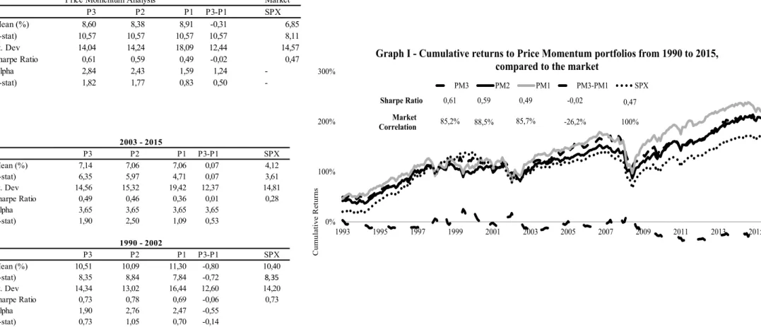
Before presenting the results of accelerated Momentum or the double sorted, I first provide a stand-alone analysis to the results yielded by Momentum strategy. Table I, found on the page below, show rank-weighted raw returns, t-statistic, standard deviation and Sharpe Ratio for Momentum alone portfolios. Between 1990 and 2015 the S&P 500 provided a total statistically significant average return of 6.85% per year and a Sharpe Ratio of 0.47.

One can perceive that all Momentum portfolios (P3, P2 and P1) yield positive, statistically significant and above market significant average annual raw returns (8.60%, 8.38% and 8.91%, respectively). This only shows the existence of Time-series Momentum proved by Moskowitz, Ooi & Pedersen (2012) - independently from being high or low momentum, using past returns as investment criteria yield on average positive and significant returns. This positive abnormal return when comparing to the market is not captured by the alphas, which by not being significant cannot show whether our portfolios are able to reject a null hypothesis of average annual abnormal returns equal to zero. In terms of risk adjusted results, we see that only P3 and P2 hold Sharpe Ratios above the market. Another particularity of Momentum is the fact that the provided portfolios seem to be highly correlated with the market (Graph I). This is not surprising given that our sample comprises stocks from S&P 500, which is also our proxy for the market.

The P3-P1 portfolio represents the investment strategy of a long position on P3 and a short on P1. Contradictory to past literature, we observe Momentum’s inexistence, i.e., despite high Momentum (PM3) stocks deliver a positive returns, low Momentum (PM1) does not imply a negative outcome, as it would be expectable by underperforming stocks. We even observe that losers (PM1) outperform winners (PM3) in terms of raw returns. However, once controlled for risk, we observe that Sharpe Ratios from P3 stocks outperform P1, reaching

(20)

15 values of 0.61 and 0.49, respectively. This means that on a risk adjusted basis, we can claim the existence of Price Momentum.

The conclusions obtained above seem to be valid historically. We verify positive, significant and above average and market cumulated returns within the two analyzed periods. Average annual returns provided by P3-P1 continue to be negative and statistically significant, claiming the inexistence of Momentum for this category. Out of the historical analysis, there are also two factors that should be mentioned: financial crisis (2000 and 2008) are highly visible on all portfolios and within our sample mostly due to the high correlation between the portfolios and the market. The second fact is that between 2003 and 2015, Sharpe Ratios have decreased significantly both in our portfolios and the market, despite reaching similar cumulated returns in both periods. The average return has fallen while on a general basis, volatility has increased. Taking a closer look, we observe that

between 1990 and 2000 the US was characterized by an economic prosperity with a constantly increasing GDP, number of jobs and low inflation. Between 1990 and 2003, there was only one crisis which stroke late in 2002/2003. Therefore, the second period, comprised between 2003 and 2015, includes the main effects of the dot.com bubble bust and the 2009 financial crisis which severely decreased returns and increased the total volatility within the stock markets.

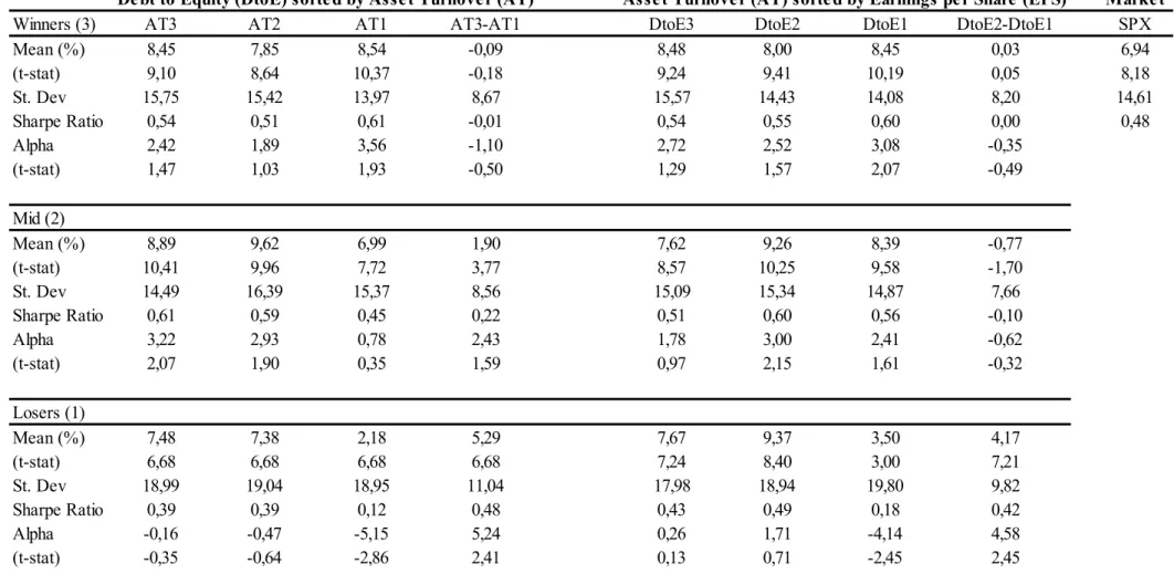
I.I.I Momentum sorted by fundamental ratios

In order to pursue a broader analysis, I also sorted Price Momentum portfolios based on Earnings Momentum. In another words, we re-ranked PM3 (winners), PM2 and PM1 (losers) into other three portfolios for each of the Earnings Momentum ratios - EPS, Current Assets/Current Liabilities, D/E, Sales/Total Assets, representing different ways of evaluating a firm’s condition: profitability, liquidity, risk and efficiency. As it was mentioned before, Momentum strategies fail to identify three different types of stocks: the ones with immediate price variation (Type One), those with delayed (Type Two) and the ones which will present a different than expected or a close to zero growth/decline (Type Three). By using fundamental ratios, our objective is to conclude whether they can serve as criteria to sort between the first and the remaining types.

(21)

16

Tables I, II and III

P3 P2 P1 P3-P1 SPX Mean (%) 7,14 7,06 7,06 0,07 4,12 (t-stat) 6,35 5,97 4,71 0,07 3,61 St. Dev 14,56 15,32 19,42 12,37 14,81 Sharpe Ratio 0,49 0,46 0,36 0,01 0,28 Alpha 3,65 3,65 3,65 3,65 (t-stat) 1,90 2,50 1,09 0,53 P3 P2 P1 P3-P1 SPX Mean (%) 10,51 10,09 11,30 -0,80 10,40 (t-stat) 8,35 8,84 7,84 -0,72 8,35 St. Dev 14,34 13,02 16,44 12,60 14,20 Sharpe Ratio 0,73 0,78 0,69 -0,06 0,73 Alpha 1,90 2,76 2,47 -0,55 (t-stat) 0,73 1,05 0,70 -0,14 1990 - 2002 2003 - 2015

Table I, II and III: Momentum Portfolio Performance Chart I: Cumulative Returns to Price Momentum Portfolios

Table I, II and III & Chart I, II and III - Tables report for stand-alone Momentum, average return, t-statistic of the return, annualized standard

deviation of the returns and the average annual Sharpe ratio. It is also presented the alphas or intercepts, and their t-statistics from a time series regression of each return series on the return of the S&P 500 index stocks. The P3-P1 portfolio represents the high minus low spread in returns. Chart I provides the cumulated returns for each portfolio compared to the market. Table and Charts II and III/ provide the same analysis split into two different periods.

Market P3 P2 P1 P3-P1 SPX Mean (%) 8,60 8,38 8,91 -0,31 6,85 (t-stat) 10,57 10,57 10,57 10,57 8,11 St. Dev 14,04 14,24 18,09 12,44 14,57 Sharpe Ratio 0,61 0,59 0,49 -0,02 0,47 Alpha 2,84 2,43 1,59 1,24 -(t-stat) 1,82 1,77 0,83 0,50

-Price Momentum Analysis

-300% -200% -100% 0% 100% 200% 300% 1993 1995 1997 1999 2001 2003 2005 2007 2009 2011 2013 2015 C umul ati ve R eturns

Graph I - Cumulative returns to Price Momentum portfolios from 1990 to 2015, compared to the market

PM3 PM2 PM1 PM3-PM1 SPX Sharpe Ratio Market Correlation 0,61 0,59 0,49 -0,02 0,47 85,2% 88,5% 85,7% -26,2% 100%

(22)

17 -300% -200% -100% 0% 100% 200% 300% 1991 1993 1995 1997 1999 2001 C umul ati ve R eturns

Graph III - Cumulative returns to Price Momentum portfolios from 1990 to 2002, compared to the market

PM3 PM2 PM1 PM3-PM1 SPX Sharpe Ratio Market Correlation 0,73 0,78 0,69 -0,06 0,73 99% 97% 94% -28% 100%

Charts II and III - Charts II and III/ provide the cumulative returns to Momentum Portfolios split into two periods: 1990-2002 and

2003-2015. -300% -200% -100% 0% 100% 200% 300% 2002 2004 2006 2008 2010 2012 2014 C umul ati ve R eturns

Graph II - Cumulative returns to Price Momentum portfolios from 2002 to 2015, compared to the market

PM3 PM2 PM1 PM3-PM1 SPX Sharpe Ratio Market Correlation 0,49 0,46 0,36 -0,01 0,28 85,2% 88,5% 85,7% -26,2% 100%

(23)

18 Therefore, we expect that for a given sole Momentum portfolio (PM3, 2 or 1), firms with high financials will outperform both the lower ones and sole Momentum. Firms with low financials as they include type 2 and 3 stocks are expected to have a lower performance than sole Momentum. If what as mentioned above occurs, the best strategy to apply is the difference between true winners and true losers (both Type One stocks).

After double sorting, generally speaking, the four analyzed ratios lead to different results. Double sorting by the Current Ratio, for all the three sole Momentum portfolios (PM3, PM2 and PM1), resulted in a decrease in average raw returns of firms with high financial ratios (CR3). We also observe a general stabilization of the same performance measurement for companies with mid (CR2) and low financials (CR1). As volatility stayed similar to sole Momentum’s, Sharpe Ratios decreased for high financials (CR3) and remained between 0.4 and 0.60 for CR2 and CR1. This states the previous hypothesis that Current ratios are outdated by market information, as it decreases the overall sole Momentum performance. Debt to Equity double sorting led to generally stable results when comparing to sole Momentum. Average Raw Returns kept between 8 and 9%. The slight increase in volatility to levels around 20%, led sometimes to small drops on Sharpe ratios. In light of what was mentioned above, we can say that the cause of these results might a positive correspondence of the information provided by the ratio and held by the market.

Therefore, we are able to conclude that both Current Ratio and Debt to Equity are not suitable criteria to solve our sole Momentum problem of distinguishing between the three types of stocks

Neither Earnings per Share seems to be, as we observe a negative spread portfolio for winners (EPS3). The same conclusions can be drawn, when comparing to the previous Debt to Equity ratio: despite a slight average return, its variation is followed by volatility, meaning that Sharpe Ratios will be kept the same. Therefore, this ratio also provides little information comparing to the one held by the market, overall performance kept stable after double sorting.

(24)

19

Table reports for the performance of Momentum portfolios re-ranked based on each stock’s fundamental ratios. The following performance measurements can be found: average return, t-statistic of the return, annualized standard deviation of the returns and the average annual Sharpe ratio. It is also presented the alphas or intercepts, and their t-statistics from a time series regression of each return series on the return of the S&P 500 index stocks. The P3-P1 portfolio represents the high

minus low spread in returns. Market

PM3 CR3 CR2 CR1 CR3-CR1 DtoE3 DtoE2 DtoE1 DtoE3-DtoE1 SPX

Mean (%) 4,80 9,67 8,53 -3,73 7,64 7,43 7,78 -0,14 6,94 (t-stat) 4,72 11,57 10,56 -5,30 9,72 8,90 8,05 -0,22 8,18 St. Dev 17,24 14,19 13,71 11,95 13,34 14,16 16,39 10,74 14,61 Sharpe Ratio 0,28 0,68 0,62 -0,31 0,57 0,52 0,47 -0,01 0,48 Alpha -1,91 4,46 3,97 -5,67 3,03 2,19 1,56 1,45 (t-stat) -0,94 2,49 1,86 -2,33 1,59 1,26 0,91 0,55 PM2 Mean (%) 4,54 8,88 8,78 -4,24 7,76 8,68 7,62 0,14 (t-stat) 4,49 9,96 11,44 -6,88 9,49 10,02 8,07 0,27 St. Dev 17,15 15,13 13,02 10,46 13,88 14,70 16,04 8,73 Sharpe Ratio 0,26 0,59 0,67 -0,41 0,56 0,59 0,48 0,02 Alpha -2,26 2,98 4,12 -6,15 2,82 2,98 1,33 1,48 (t-stat) -1,30 1,60 2,58 -3,36 1,65 1,80 0,65 1,09 PM1 Mean (%) 7,31 7,17 8,64 -1,33 7,73 6,84 8,83 -1,10 (t-stat) 5,24 5,74 7,10 -1,45 6,15 5,55 6,84 -1,34 St. Dev 23,67 21,20 20,65 15,48 21,33 20,92 21,93 14,00 Sharpe Ratio 0,31 0,34 0,42 -0,09 0,36 0,33 0,40 -0,08 Alpha -1,43 -0,76 1,27 -2,67 -0,03 -0,47 0,57 -0,60 (t-stat) -0,61 -0,46 0,31 -0,81 -0,18 -0,38 0,18 -0,33

Price Momentum sorted by Debt to Equity (DtoE) Price Momentum sorted by Current Ratio (CR)

PM3 AT3 AT2 AT1 AT3-AT1 EPS3 EPS2 EPS1 EPS2-EPS1

Mean (%) 8,20 7,69 7,91 0,29 6,27 7,63 8,78 -2,51 (t-stat) 9,52 8,56 9,13 0,51 7,19 9,42 9,53 -4,27 St. Dev 14,61 15,25 14,70 9,57 14,80 13,74 15,64 9,99 Sharpe Ratio 0,56 0,50 0,54 0,03 0,42 0,55 0,56 -0,25 Alpha 2,73 1,80 2,67 0,06 1,10 2,46 2,80 -1,66 (t-stat) 1,76 0,98 1,12 0,49 0,66 1,38 1,66 -0,78 PM2 Mean (%) 6,99 9,05 5,98 1,01 7,59 8,81 7,39 0,20 (t-stat) 7,93 9,56 6,92 1,97 9,11 10,58 7,70 0,41 St. Dev 14,95 16,07 14,67 8,68 14,13 14,13 16,28 8,37 Sharpe Ratio 0,47 0,56 0,41 0,12 0,54 0,62 0,45 0,02 Alpha 1,12 2,92 0,33 0,78 2,20 3,36 1,09 1,10 (t-stat) 0,83 1,47 0,17 0,58 1,46 2,19 0,51 0,85 PM1 Mean (%) 8,22 10,09 4,95 3,27 10,85 8,95 6,58 4,27 (t-stat) 6,70 8,13 3,91 4,91 10,25 7,22 4,67 5,88 St. Dev 20,81 21,07 21,51 11,30 17,97 21,05 23,92 12,35 Sharpe Ratio 0,40 0,48 0,23 0,29 0,60 0,43 0,27 0,35 Alpha 0,38 2,06 -2,74 3,20 4,33 0,87 -2,36 6,83 (t-stat) 0,15 0,64 -1,20 1,57 1,86 0,25 -1,12 3,16

(25)

20

Chart IV, V and VI: Momentum Portfolio Performance double sorted by Asset Turnover, Earnings per Share, Current Ratio & Debt to Equity

Charts report for the cumulated returns to top performers of price Momentum portfolios double sorted by Asset Turnover (AT), Earnings per Share (EPS), Current Ratio (CR) or Debt to Equity ratio (DtoE).

Graph IV - Cumulative returns to top performers of Price Momentum portfolios double sorted by Asset Turnover from 1990 to 2015, compared to the market

PM3 PM3A3 PM2A2 PM1A2 SPX

Sharpe Ratio Market Correlation 0,73 0,56 0,48 85% 83% 83% 0,48 1% 0,56 83% -400% -300% -200% -100% 0% 100% 200% 300% 400% 1992 1994 1996 1998 2000 2002 2004 2006 2008 2010 2012 2014 C umul ati ve R eturns

Graph V - Cumulative returns to top performers of Price Momentum portfolios double sorted by Earnings Per Share from 1990 to 2015, compared to the market

PM3 PM3 EPS1 PM2 EPS2 PM1 EPS3 SPX

Sharpe Ratio Market Correlation 0,73 0,56 0,62 0,60 85% 84% 85% 80% 0,48 1%

(26)

21

Charts report for the cumulated returns to top performers of price Momentum portfolios double sorted by Asset Turnover (AT), Earnings per Share (EPS), Current Ratio (CR) or Debt to Equity ratio (DtoE).

Graph VI - Cumulative returns to top performers of Price Momentum portfolios double sorted by Current Ratio from 1990 to 2015, compared to the market

Sharpe Ratio Market Correlation 0,73 0,31 0,42 0,29 85% 81% 78% 30% 0,26 1% -300% -200% -100% 0% 100% 200% 300% 1992 1994 1996 1998 2000 2002 2004 2006 2008 2010 2012 2014 C umul ati ve R eturns

Graph VII - Cumulative returns to top performers of Price Momentum portfolios double sorted by Debt to Equity Ratio from 1990 to 2015, compared to the market

Sharpe Ratio Market Correlation 0,73 0,21 0,23 0,24 85% 0,83% 80% 32% 0,48 1%

(27)

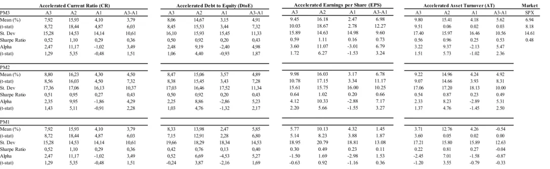
22 Regarding average raw returns, Momentum combined with Asset Turnover generated heterogeneous conclusions among the different Price Momentum portfolios (PM3, 2 and 1), when comparing to sole Momentums’. Our expected results were partially verified after double sorting for Asset Turnover ratio; instead of increasing returns for high AT (AT3) they remained fairly stable; meaning that for those stocks AT adds no extra value to Momentum. However, for mid performers (PM2) and Price Momentum losers (PM1) portfolios with low AT (AT1s) decreased its performance, leading to positive spread portfolios (PMx AT3 – PMx AT1). This takes us to conclude that AT seems to be a positive but weak identifier of firms which will have future decreasing revenues (overvalued stocks), delayed or stabilizing price reactions for Price Momentum losers and Mid Performers.

The same conclusions can be drawn if we split or time frame into two: 1990-2002 and 2003-2015 (Table IV.I and VI.II, respectively on appendix6)

II.I.II Accelerated Momentum

Following Bird & Casavecchia (2007)’s methodology, stocks were double sorted according to its recent Momentum’s growth rate – last 3 months versus 12 or 12 over 24, depending if the stock has a high or low Momentum. Results are available on table III and chart VII. I expected that within each sole Momentum portfolio, firms with high acceleration (A3) provide higher returns than lower ones (A1) and sole Momentum. In this way, we expect to be able to isolate true winners (Type One) on A3 and the remaining (Type Two and Three) on the remaining portfolios (A2 and A1). True losers should be isolated in A1 portfolios, as they seem to provide low returns with low short-term trend. Therefore, if the acceleration phenomenon is verified, PM3 A3 – PM1 A1 (true winners – true losers) will be the best combination.

In fact, that is what we observe for high and mid Momentum stocks (PM3 and PM2). Average annual returns increased for accelerated winners (A3) to above 27% while losers (A3) provide negative up to 15% p.a. Therefore, best case scenario, if we long A3 and short A1 stocks (spread portfolio) for Price Momentum winners (PM3), we obtain a higher return (on average 40% p.a.) and Sharpe ratio (2.26) than any individual strategy, sole Momentum and the

(28)

23 Market. Therefore, we are able to say that this strategy successfully separates Type Two and Three assets from Type one within Momentum Winners (PM3) and Mid Performers (PM2). Moreover, being long on A3 and short on A1 provides our portfolio with a negative correlation to the market (-18%), as perceived on chart VII. This would be expected given that the ideal strategy should prove itself resilient to crashes as it is supposed to pick the stocks with a greater growth (Type One) and decline (Type Three) in stock price returns, even when the market is crashing.

Within Price Momentum loser stocks (PM1) the acceleration index seems to have the reverse effect – assets with low acceleration yielded a very positive return (PM1 A1) of 15% - both above market and above sole Momentum. Also, within the same portfolio, high acceleration assets provided a negative 0.61% outcome and a Sharpe Ratio close to zero. This allows us to take two conclusions: (1) truly worse performers are the ones with low past performance but higher acceleration (PM1 A3) – even though they seem to be recovering, they end up decreasing in the longer term, leading to negative annual returns. The second conclusion (2) is that when comparing to sole Momentum, stocks with the lowest performance and acceleration (PM1 A1) bring both future higher average returns (15%) and Sharpe ratios (0.68). In fact, Bondt & Thaler (1985) confirm these results as they conclude that there is a natural tendency for investors to be over-pessimistic regarding current losers. Therefore, investing on current losers with lowest acceleration (PM1 A1) takes advantage of this behavioral bias, profiting from the stock price reversal. Therefore, among price momentum losers (PM1) the best alternative is investing on low momentum and acceleration (PM1 A1) and short the true losers (PM1 A3).

This strategy is therefore able to sort correctly truly growing stocks (Type One) and overvalued stocks (Type Three) for Price Momentum winners (PM3). For losers (PM1), it identifies the ones which are undervalued and the overvalued. This leads in both cases for high, positive and above market returns. In this case, we verify that the true winners (PM3 A3) minus true losers (PM1 A3) is not the best performing portfolio. It seems that investing on true winners (PM3 A3) and shorting false ones (PM3 A1) would be the best possible combination.

(29)

24

Table VIII: Accelerated Momentum portfolios performance

Chart VII: Cumulated returns of Spread Accelerated Mometum Portfolios

Table reports for the performance of Momentum portfolios re-ranked based on each stocks’ acceleration ratios. The methodology used was the one provided by Bird & Casavecchia (2007). According to the same authors, positive trends take longer to be identified than negative ones. Therefore, the 50% higher Momentum stocks were accelerated based on a long term ratio between Momentum (12 months over 24) and the remaining using a short term one (3 months over 6). Then stocks within each portfolio (PM3, PM2 and PM1) were double sorted based on the value of the ratio obtained leading to a total of 9 (3x3) new portfolios (PMx A3, PMx A2 and PMx A1)

The following performance measurements can be found: average return, t-statistic of the return, annualized standard deviation of the returns and the average annual Sharpe ratio. It is also presented the alphas or intercepts, and their t-statistics from a time series regression of each return series on the return of the S&P 500 index stocks. The P3-P1 portfolio represents the high minus low spread in returns.

Chart VII presents the cumulated returns for the top performers of Accelerated Momentum portfolios Market PM3 A3 A2 A1 A3-A1 SPX Mean (%) 27,74 23,59 -15,84 43,58 10,41 (t-stat) 10,36 8,43 1,87 12,63 0,06 St. Dev 14,86 15,21 18,99 19,32 14,26 Sharpe Ratio 1,87 1,55 -0,83 2,26 0,73 Alpha 23,38 16,58 -23,56 59,74 (t-stat) 5,27 4,46 -6,29 7,73 PM2 Mean (%) 20,40 17,91 -5,78 26,19 (t-stat) 13,48 12,28 -3,58 26,51 St. Dev 16,37 15,78 17,47 10,68 Sharpe Ratio 1,25 1,13 -0,33 2,45 Alpha 14,86 10,58 -12,17 30,41 (t-stat) 3,71 3,64 -3,10 5,29 PM1 Mean (%) -0,61 13,55 18,91 -19,35 (t-stat) -0,37 8,93 12,50 -15,78 St. Dev 21,14 19,66 19,61 15,90 Sharpe Ratio -0,03 0,69 0,96 -1,22 Alpha -10,44 4,16 9,80 -18,45 (t-stat) -2,10 0,88 1,92 -3,87

Table V: Accelerated Price Momentum

-900% -650% -400% -150% 100% 350% 600% 850% 1992 1994 1996 1998 2000 2002 2004 2006 2008 2010 2012 2014 C umul ati ve R eturns

Graph VII - Cumulative returns to Spread Accelerated Price Momentum portfolios 1990 to 2015, compared to the market

PM3 PM2A3 - PM2A1 PM3A3 - PM3A1 PM1A3 - PM1A1 SPX

Sharpe Ratio Market Correlation 0,73 2,26 2,45 -1,22 85% 18% 7% 3% 0,48 1%

(30)

25 However, identifying correctly Type One, Two and Three stocks creates the following best investment strategy: within stocks with high momentum (PM3), invest in true winners and short false winners (PM3 A3 – PM3 A1). For stocks with low momentum (PM1), one should invest on those with low acceleration (PM1 A1) – false losers - and short the ones with high – true losers (PM1 A3). This would yield a total average annual return around 60%.

On an historical perspective, we observe that the period before the Dot.com bubble burst boosted our strategy’s returns of investing on winner stocks with high acceleration, shorting winners with low acceleration (PM3 A3 - PM3 A2) and investing on losers with low acceleration – PM1A1 (Chart VII, VIII and VIII – last two in exhibit). A possible explanation is that this phenomenon is driven by short term results that compose a speculating bubble. In another words, during those periods, investors seem to be more risk prone, putting their money in more volatile stocks that provide high immediate returns, increasing those assets’ acceleration, they can be called “trend chasers” (De Long et al (1990)). If we take in consideration the whole market, we might observe a phenomenon where there are higher than normal number of stocks “in trend” with very high accelerations. Once the bubble bursts, our strategy does not suffer severely from the crisis because it is able to detect decreases in investments by the drop in acceleration ratios, even though it decreased its average growth rate. We also see this type of results, even though in a much smaller scale on the 2008 sub-prime crisis.

II.II Earnings Momentum

As mentioned above, Earnings Momentum is a strategy fully based on firms’ financials. Our hypothesis is that companies presenting the best financial health are the ones holding a higher future return. In order to perform this analysis, we used four different ratios evaluating four different critical areas for any firm: Profitability (Earnings per Share - EPS), Liquidity (Current Ratio – current assets/current liabilities), Risk (Debt-to-equity – D/E) and Efficiency (Asset Turnover – Sales/Total Assets). I not only provide a single but also a double sorting, since one ratio might not representative of the whole firm condition.

Results obtained from Earnings Momentum sole revealed two different conclusions:

Debt to Equity (DtoE) and Current Ratio (CR) provided not significant results, in general. This means that we cannot prove both annual average and abnormal returns different from

(31)

26 zero and therefore, these two criteria are not useful on a standalone basis to obtain positive and above market returns. One can interpret these results by saying that the information included on these ratios is fully reflected in the market prices, leading to indifferent reactions after sorting.

Using Asset Turnover (AT) and Earnings per Share (EPS) as criteria to allocate assets to portfolios yield similar and positive average annual returns across winners (AT3 and EPS3), mid performers (AT2 and EPS2) and losers (AT1 and EPS1) - between 6% and 9%. Despite being slightly higher than the market, the increase in volatility dropped Sharpe ratios to S&P 500’s levels (between 0.4 and 0.6). Alphas also point the existence of positive and abnormal returns when compared to the index. Considering these results, high correlation observed on Chart X was expectable because I used S&P 500’s past and present stocks both as sample and benchmark and this strategy was not able to select persistently the true winners (Type One). Concluding, we verify that sorting portfolios by efficiency (AT) and profitability (EPS) can lead to positive and similar to market returns. However, the same problem as Momentum is verified: this strategy does not have the ability to distinguish between winners (Type One) and losers (Type Three) stocks, as similar results are provided across portfolios. I also observe that among AT and EPS sorting, there is a winner-loser spread between the risk adjusted returns. This suggests that despite offering similar average annual returns, stocks with lower financial ratios (EPS1/AT1) tend to be more volatile than the ones with higher.

Also, we observe that Sole Earnings Momentum based on AT or EPS yield similar outcomes both in terms of average returns (between 8 and 9%) and Sharpe Ratios (between 0.5 and 0.6), when comparing to Price Momentum. I also find that both strategies (Earnings and Price Momentum) provide a very high correlation to the market (greater than 80%), suggesting they are much correlated to each other. This similarity in returns and correlation, leads us to presume that firms with high financials also have high past return. As we have seen above, within our sample, each firms’ past returns seems to explain the future outcomes (Moskowitz, Ooi & Pedersen (2012)). If this holds, it can be the reason why all Earnings Momentum portfolios sorted by AT and EPS yield high returns among most of the portfolios.

(32)

27 <

Chart X: Top Earnings Momentum Portfolios Cumulated Performance

Table reports for the performance of Earnings Momentum stocks’. Portfolios were ranked based on each firms’ fundamental ratios. The following performance measurements can be found: average return, t-statistic of the return, annualized standard deviation of the returns and the average annual Sharpe ratio. It is also presented the alphas or intercepts, and their t-statistics from a time series regression of each return series on the return of the S&P 500 index stocks. The EM3-EM1 portfolio represents the high minus low spread in returns.

Chart reports the Top Earnings Momentum portfolio’s cumulated performance

Market

PM3 CR3 CR2 CR1 CR3-CR1 DtoE3 DtoE2 DtoE1 DtoE3-DtoE1 SPX Mean (%) 8,79 8,85 6,73 2,06 5,50 6,79 6,24 -0,74 6,94 (t-stat) 0,03 0,03 0,02 0,02 5,75 0,02 0,02 -0,01 8,18 St. Dev 15,58 16,35 15,47 7,05 16,80 16,46 17,13 7,02 14,61 Sharpe Ratio 0,56 0,54 0,43 0,29 0,33 0,41 0,36 -0,10 0,48 Alpha 2,22 1,74 0,08 2,13 -1,56 -0,19 -1,05 -0,51 (t-stat) 1,60 1,39 0,06 1,48 -1,04 -0,13 -0,72 -0,36

CR3 CR2 CR1 CR3-CR1 EPS3 EPS2 EPS1 EPS2-EPS1 Mean (%) 6,23 9,03 8,18 -1,94 8,70 8,77 8,17 0,54 (t-stat) 0,02 0,03 0,03 -0,01 10,76 10,53 7,99 1,05 St. Dev 18,84 15,44 13,99 10,87 14,20 14,62 17,93 8,99 Sharpe Ratio 0,33 0,58 0,58 -0,18 0,61 0,60 0,46 0,06 Alpha -1,89 2,53 2,50 -4,29 2,92 2,48 0,37 2,55 (t-stat) -1,26 1,82 1,76 -2,26 2,06 2,09 0,26 1,55

Earnings Per Share (EPS) Current Ratio (CR)

Asset Turnover (AT) Debt to Equity (DtoE)

-300% -150% 0% 150% 300% 1992 1994 1996 1998 2000 2002 2004 2006 2008 2010 2012 2014 C um ul at ive R et ur ns

Graph X - Cumulative returns to top performing Earnings Momentum portfolios from 1990 to 2015, compared to the market

PM3 AT2 CT2 DtoE2 EPS2 SPX

Sharpe Ratio Market Correlation 0,73 0,60 0,58 0,41 85% 93% 90% _88% 0,48 1% 0,60 92%

(33)

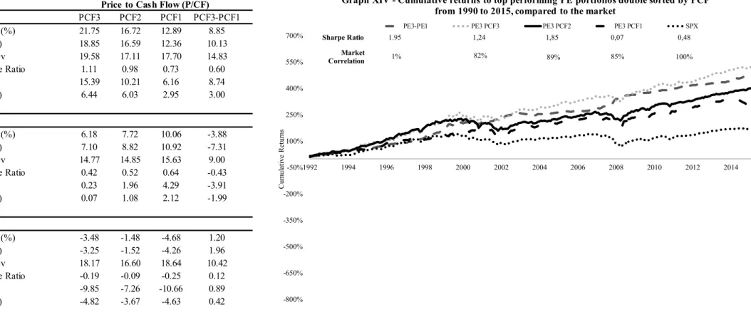
28 II.II.I Double Sorted Earnings Momentum

Double sorting by Earnings Momentum means trying to find the best combination of financial ratios that include information that is not yet absorbed by the market (investor under reaction). Assuming that prices will correct to financial based information, it is expected to provide useful insights to predict future returns. Results provided by double sorted earnings Momentum can be found on Chart XI and tables XI, XIII, XIV, XV and XVI (last four provided on appendix). The map of results and expectations can be found below on table XII. As we concluded above, information provided by DtoE and CR seem to be fully absorbed by the market. Therefore, we expect that double sorting using these ratios would lead to similar results as not doing it and double sorting these ratios by the other variables will increase its explanatory power. As it can be observed on the table below, for DtoE and CR expectations almost matched the results. Average annual returns grew to normal values (between 7 and 9%) and Sharpe Ratios comprised within 0.4 and 0.6)

Like we were expecting, after double sorting the significant variables (AT and EPS) by the irrelevant ones (DtoE and CR), results stayed similar to the single sorted ones.

Surprisingly we found that Debt to Equity and Current Ratio have a greater explanatory power when combined when comparing to sole performance. Solely they are insignificant but together they yield positive, significant and sometimes above market returns (Table XIII & XIV). Average annual returns yielding returns between 6 and 9% with similar to market Sharpe Ratios (0.49) DtoE CR AT EPS DtoE x i | nv nv | nv nv | nv CR i | nv x nv | nv nv | nv AT g | g to nv g | g to nv x g | nv EPS g | g to nv g | g to nv g | nv x Single Sorting Double Sorting

Table XII - Map of Results & Expectations

Table below compares the expectation versus the reality (Expectation | Reality) in light of the results obtained by single sorting - dark grey means they matched. The following legend can be used to interpret results: nv = normal values similar to single sorting; i = insignificant; ss = double sorting equals single sorting; g = growth in the explanatory power; d = decrease in explanatory power.