Operation of a fuel cell with biohydrogen obtained from food waste

(1)

UNIVERSIDADE DE LISBOA FACULDADE DE CIÊNCIAS

DEPARTAMENTO ENGENHARIA GEOGRÁFICA, GEOFÍSICA E ENERGIA

Operation of a fuel cell with biohydrogen obtained from food

waste

Pedro Nuno Pires Farrancha

Mestrado Integrado em Engenharia da Energia e do Ambiente

Trabalho de Projeto orientado por: Carla Silva (FCUL)

Patricia Moura (LNEG)

(2)

ii

Abstract

In the current world where alternative and responsible energy supply is required, this project focus on studying the viability of biohydrogen produced from dark fermentation of food waste, in a polymer electrolyte membrane fuel cell.

A fuel cell Parker with one cell and active area of 10.89 cm2 was integrated in a closed system and connected to a balloon to feed gas in the circuit. This system was created to study the cell performance as temperature and gas purity varied. Several tests were made with industrial hydrogen (100% purity) and biohydrogen (98% purity) at 25°C and 50°C. The results showed small variations between the conditions applied. The biohydrogen had similar behaviour to industrial hydrogen, which points that it has a high hydrogen concentration, and could be used as an alternative to fuel this technology.

In this small scale study, the maximum energy generated per hydrogen litre was 1.593 Wh/L, with fuel cell efficiency of 0.529 and current values of 11.02 mA/cm2_{for a total}

of 45.047 L of biohydrogen produced.

Keywords: Proton exchange membrane fuel cell (PEMFC), biohydrogen, food waste, polarization curve.

(3)

iii

Resumo Alargado

Vivemos numa era em que existe uma clara sobre utilização de recursos. Para além disso, é de notar também, um crescimento da população mundial a um elevado ritmo e o aparecimento de novos hábitos de consumo, o que agrava a forma como são geridos os nossos recursos. E neste contexto que surge o desperdício alimentar que, já sem qualquer valor enquanto alimento para o ser humano, tem diversos outros tipos no qual se pode valorizar.

Uma necessidade básica e adquirida pelo ser humano, com tendência também para aumentar é o consumo de energia, sendo este cada vez mais urgente de suprir de forma sustentável.

Uma combinação entre a necessidade e o recurso disponível em excesso, e utilizando a tecnologia da pilha de combustível, originou o tema desta dissertação “Operation of a

fuel cell with biohydrogen obtained from food waste”. Na pilha de combustível é

fornecido hidrogénio biológico obtido a partir da fermentação escura de um lote de desperdício alimentar. O objectivo deste trabalho é estudar o comportamento deste gás na pilha de combustível.

O circuito para o estudo deste gás na pilha de combustível foi construído de raiz. Uma célula de combustível de membrana de troca de protões com área activa de 10.89 cm2 foi integrada num sistema fechado e alimentado por um balão de gás que introduz o combustível no circuito. Este sistema foi criado para estudar a performance da célula com a variação de temperatura e pureza do gás. Como forma de comparação, foram realizados testes com hidrogénio industrial e biohidrogénio ambos a 25°C e 50°C. A análise deste gás durou enquanto o mesmo foi produzido no processo de fermentação escura, correspondente a um período de cerca de 14 dias, onde foram produzidos cerca de 45 litros de gás em condições PTN. Durante este tempo, o gás foi sendo armazenado em balões próprios para armazenar hidrogénio, e imediatamente utilizados na pilha de combustível. Foram estudados nove lotes de gás e um de hidrogénio industrial. Cada lote de gás foi estudado e repetido entre duas a quatro vezes.

Os resultados mostraram pequenas variações entre as condições aplicadas. O bio-hidrogénio teve um comportamento similar com o bio-hidrogénio industrial, o que aponta que tem uma elevada concentração de hidrogénio e que pode ser usado como alternativa para esta tecnologia. No total de 45 litros de gás produzidos, com um fluxo de produção de gás de aproximadamente 133 mL/h, de acordo com o fluxo de produção de energia a partir da pilha de combustível (1.59Wh/L), seria possível produzir cerca de 71.76Wh com este sistema e tecnologia utilizada e com valores de eficiência de aproximadamente 63%.

Palavras-chave: Pilha de combustível de membrana de troca protónica (PEMFC), biohidrogénio, desperdício alimentar, curva de polarização.

(4)

iv

Index

Abstract ... ii

Resumo Alargado ... iii

List of figures ... vi

List of tables ... vi

Acronyms, Nomenclature and Units ... vii

1Introduction ... 10

1.1 Context and Motivation ... 10

1.2 Objective ... 11

2 Literature Review ... 12

2.1 Hydrogen production methods ... 12

Biohydrogen production ... 12

Dark fermentation biohydrogen to fuel cell ... 13

2.2 Fuel Cell technology ... 13

Molten Carbonate FC (MCFC) ... 14

Solid Oxide FC (SOFC) ... 14

Alkaline FC (AFC) ... 14

Phosphoric Acid FC (PAFC) ... 14

Direct Methanol FC (DMFC) ... 14

Proton Exchange Membrane FC (PEMFC) ... 14

2.3 Current applications of FCT ... 15 2.3.1 Transport sector ... 15 2.3.2 Portable applications ... 16 2.3.3 Stationary applications ... 16 2.3.4 Other applications ... 16 2.4 Other studies ... 16 2.4.1 Temperature influence... 16

2.4.2 Gas purity influence ... 16

3 Methods ... 18

3.1 Theoretical concepts ... 18

3.1.1 Thermodynamics ... 18

3.1.2 Polarization curve ... 20

3.2 Fuel Cell assembly and components ... 21

3.2.1 Materials ... 21

(5)

v

3.3 PEM Fuel Cell procedure ... 23

4 Results and Analysis ... 25

4.1 Obtained data ... 25

4.2 Efficiency ... 28

4.2.2 Energy generated ... 29

5 Conclusions and future recommendations ... 31

6 References ... 32 7 Appendix ... 33 7.1 Trial 1, 16/out ... 33 7.2 Trial 2, 19/out ... 35 7.3 Trial 3, 23/out ... 36 7.4 Trial 4, 24/out ... 37 7.5 Trial 5, 25/oct ... 39 7.6 Trial 6, 26/out ... 40 7.7 Trial 7, 29/oct ... 41 7.8 Trial 8, 30/oct ... 43 7.9 Trial 9, 31/oct ... 44

(6)

vi

List of figures

Figure 1 Hydrogen sources, production and end-use technologies 8 ... 12

Figure 2 Some characteristics of major fuel cell types 16 ... 15

Figure 3 Typical polarization curve of a fuel cell 16 ... 20

Figure 4 Typical power curve and polarization curve 26 ... 21

Figure 5 PEMFC. 1-Assembled fuel cell and connected to the circuit. 2/3/4- FC during assembly. a-Electrolyte membrane, b-Teflon gasket, c-Graphite Composite Plate, d-Molded plastic endplate, e-Nickel-coated brass current collector. ... 22

Figure 6 Picture of the circuit created to test the biohydrogen. A-Parker TekStak Fuel Cell with graphite electrodes and platinum-rhodium electrolyte, B-Potentiometer, C-Voltmeter, D-Ammeter, E-Power source, F-Gas balloon, G-Air pump for gas, H-Air pump, I-Air washing bottle, J-Gas washing bottle, K-Water bath. ... 22

Figure 7 Schematic representation of the electric and gaseous circuit. A-Parker TekStak Fuel Cell with graphite electrodes and platinum-rhodium electrolyte, B-Potentiometer, C-Voltmeter, D-Ammeter, F-Gas balloon, G-Air pump for gas, H-Air pump, I-Air washing bottle, J-Gas washing bottle, K-Water bath. ... 23

Figure 8 All obtained values of current and voltage throughout the whole study... 25

Figure 9 iV curve of the average of interpolations in the same conditions of Test8_50. 27 Figure 10 Polarization curve and power curve, all values per cm2. ... 27

Figure 11 Efficiency values for all trials, including control test with industrial hydrogen (10) ... 28

Figure 12 iV curves of averaged interpolated trial 1 values at each temperature ... 35

Figure 21 iV curves of averaged interpolated trial 10 (industrial hydrogen) values at each temperature ... 46

List of tables

Table 1 Current and potential of 3 rehearsals with the same gas at 50°C 26

Table 2 Interpolated values of table 1 26

Table 3 Current, potential, standard error values and power measured in Test8_50 26 Table 4 Values of various parameters of the Test8_50 iV curve. 28 Table 5 Power values for total generated fuel consumption 29 Table 6 Final values of energy produced with FC rate and DF rate as well as the generation

per litre of bio-gas. 30

Table 7 Obtained voltage and current data of Trial 1 at 25°C (3 repetitions) 34 Table 8 Obtained voltage and current data of Trial 1 at 50°C (2 repetitions) 34 Table 9 Average of interpolated values of trial 1 at each temperature 34 Table 10 Obtained voltage and current data of Trial 2 at 25°C (4 repetitions) 35

(7)

vii Table 11 Obtained voltage and current data of Trial 2 at 50°C (4 repetitions) 35 Table 12 Average of interpolated values of trial 2 at each temperature 36 Table 13 Obtained voltage and current data of Trial 3 at 25°C (4 repetitions) 36 Table 14 Obtained voltage and current data of Trial 3 at 50°C (3 repetitions) 37 Table 15 Average of interpolated values of trial 3 at each temperature 37 Table 16 Obtained voltage and current data of Trial 4 at 25°C (3 repetitions) 38 Table 17 Obtained voltage and current data of Trial 4 at 50°C (3 repetitions) 38 Table 18 Average of interpolated values of trial 4 at each temperature 38 Table 19 Obtained voltage and current data of Trial 5 at 25°C (4 repetitions) 39 Table 20 Obtained voltage and current data of Trial 5 at 50°C (3 repetitions) 39 Table 21 Average of interpolated values of trial 5 at each temperature 40 Table 22 Obtained voltage and current data of Trial 6 at 25°C (2 repetitions) 40 Table 23 Obtained voltage and current data of Trial 6 at 50°C (2 repetitions) 41 Table 24 Average of interpolated values of trial 6 at each temperature 41 Table 25 Obtained voltage and current data of Trial 7 at 25°C (4 repetitions) 42 Table 26 Obtained voltage and current data of Trial 7 at 50°C (3 repetitions) 42 Table 27 Average of interpolated values of trial 7 at each temperature 42 Table 28 Obtained voltage and current data of Trial 8 at 25°C (3 repetitions) 43 Table 29 Obtained voltage and current data of Trial 8 at 50°C (3 repetitions) 43 Table 30 Average of interpolated values of trial 8 at each temperature 43 Table 31 Obtained voltage and current data of Trial 9 at 25°C (2 repetitions) 44 Table 32 Obtained voltage and current data of Trial 9 at 50°C (2 repetitions) 44 Table 33 Average of interpolated values of trial 9 at each temperature 45 Table 34 Obtained voltage and current data of Trial 10 (industrial hydrogen) at 25°C (3

repetitions) 45

Table 35 Obtained voltage and current data of Trial 10 (industrial hydrogen) at 50°C (3

repetitions) 45

Table 36 Average of interpolated values of trial 10 (industrial hydrogen) at each

temperature 46

Acronyms, Nomenclature and Units

A(cm2) – Area (Square Centimeter) AFC – Alkaline Fuel Cell

CHP – Cogeneration of Heat and Power CO – Carbon Monoxide

CO2 – Carbon Dioxide

DF – Dark Fermentation

(8)

viii e- - electron

E(J) – Energy (Joule) F - Faraday’s Constant FC - Fuel Cell

FCT – Fuel Cell Technology FCV – Fuel Cell Vehicle H+ - Hydrogen ion H2 – Hydrogen molecule

H2O – Water

H2S - Hydrogen Sulfide

I(A) – Current (Amper)

MCFC - Molten Carbonate Fuel Cell MEA – Membrane Electrode Assembly n(mol) – Quantity (mol)

NH3 – Ammonia

O2 – Oxygen

Ocv – Open Circuit Voltage p(atm) – Pressure (Atmosphere) P(W) – Power (Watt)

PAFC - Phosphoric Acid Fuel Cell

PEMFC - Proton Exchange Membrane Fuel Cell PV – Photovoltaic

R – Ideal Gas Constant

R&D – Research and Development R(ohm) – Resistance (ohm)

SOFC - Solid Oxide Fuel Cell

T(°C) – Temperature (Degrees Celsius) T(h) – Time (hour)

UAV – Unmanned Aerial Vehicle UUV - Unmanned Undersea Vehicles

(9)

ix V(L) – Volume (Litre)

V(V) – Voltage (Volt)

ΔG – Gibbs Energy Variation ΔH – Enthalpy Variation

(10)

10

1Introduction

1.1 Context and Motivation

The increasing numbers of human population reached a point where the resources are not enough for everyone. In 1960 the world population was around 3 billion people. In 1999 it doubled to 6 billion. In 2019 we are going to reach 7.7 billion and in 2045 it is estimated 9.5 billion, more than triple regarding to 1960 1. Resource consumption and environmental degradation are linked to population growth, and accelerated by consumption habits, some technological developments, social organization and resource management. There are many direct and indirect consequences of these actions, such as loss of biodiversity, raising sea level, increasing greenhouse gases emissions and global temperature, uncertain atmospheric events (floods, draughts, acid rains) among many others 2. Thus, human is the main responsible for all these actions. Behaviours and mentalities must change drastically. Living a sustainable life should not be an option, but a need, an obligation. On average, a person uses three times more resources than it should. In a world-wide scale, human population is using three times the resources available on Earth. This means that there would need to be three Earths available to supply all the current demand 3. So, it is vital to change mentalities regarding overconsumption and adapt our actions to the world we live in. Then, we must supply our needs in a responsible way.

Waste is the output of a system which usually is not valued, but some kinds of biodegradable waste may be used as substrate in agriculture or other applications and valued like any other resource. In Europe alone, 88 million tons of food are wasted every year 4. Although the processes of production, distribution and consumption of food may be optimized, it is likely that there will always be a loss. Food waste production is a consequence of population increase and new consumption habits and could at the same time be valued into electricity and sometimes heat, while properly managing this resource. There are several ways to value this waste by incinerating, composting or digesting.

Analysing the current energy transition that is undergoing, a lot of alternatives to fossil fuels are under R&D. Photovoltaic (PV) technology is growing exponentially and there is still a lot of growing potential. The electric car for instance is being developed and evolving, but technology is constantly growing and there are good indicators that point out that electric fuel cell (FC) cars are going to have its share in the market. There are already some commercially available FC cars, from Honda, Hyundai and Toyota 5. FC technology is seen as the potential future for transport applications and is expanding already to other industries, as seen in Walmart case study (forklifts are being powered with FC technology) 6. The current limitation of this technology is the hydrogen (H2)

source for the conversion from H2 to electricity. Currently this technology is being

promoted as clean and renewable, but the main source of this gas has a huge carbon footprint. Around 98% of the hydrogen is obtained from steam reforming of oil or natural gas and coal gasification 7. Thus, sustainable sources to obtain this gas are needed. This need, associated with the high levels of waste production, may be combined and waste

(11)

11 becomes the source for sustainable biohydrogen production. This project will then test the viability of the biologically produced hydrogen in the fuel cell.

1.2 Objective

The objective of this study was to integrate a PEMFC with a bioreactor and evaluate its viability and behaviour in terms of temperature and hydrogen purity. A small-scale proton-exchange membrane fuel cell (PEMFC) was operated with the biohydrogen produced and industrial hydrogen, as a comparison basis. Both gases at 25°C and 50°C. All the circuit that regards electricity production was built from scratch where it was assembled a Parker fuel cell from TekStakTM Educational Fuel Cell Kit with graphite composite plates and a MEA(membrane electrode assembly) composed by platinum catalysts and a proton exchange membrane made from Nafion.

(12)

12

2 Literature Review

2.1 Hydrogen production methods

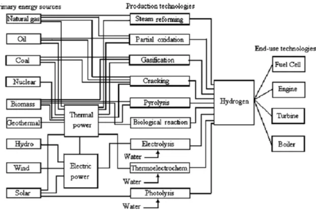
There are several ways to produce hydrogen. Figure 1 summarizes its source, production technologies and conversion technologies to electric energy. The most recurrent sources for hydrogen production are natural gas reforming (50%), oil reforming (30%), coal gasification (18%), water electrolysis (1.9%) while other sources (such as biological) represent only (0.1%) 7_.

Figure 1 Hydrogen sources, production and end-use technologies 8

Biohydrogen production

The conversion of hydrogen into electric energy releases H2O as its only sub product.

This means that this is a carbon free process, and sometimes misinterpreted and seen as completely carbon free fuel. But when an upstream analysis is made, this hydrogen comes from fossil fuels as shown in the previous chapter. To take advantage of this energy carrier as a clean and non-polluting source, it must come from renewable methods. Since hydrogen is the most abundant element on earth, research and development is needed to extract this element from as maximum sources as possible. There are several ways to produce biohydrogen such as biophotolysis, photofermentation and dark fermentation 9. To support the biohydrogen obtention method Rahman, et al says that from these 3 biological processes, “The dark fermentation process is the most beneﬁcial and proﬁtable

as it does not need light energy as in light fermentation” 9. Which means this process

(13)

13 Biophotolysis is a light dependent process that uses microalgae and cyanobacteria photosynthetic processes to split water into hydrogen. The maximum rate of H2

production is between 0.05 and 30 mL/Lh9_.

Photofermentation is another light dependent process that uses photosynthetic bacteria to convert organic matter into biohydrogen and its maximum rate varies between 1 and 102.33 mL/Lh9.

Dark fermentation is a light independent and anaerobic process that uses different carbohydrates according to the bacterial strain present, such as glucose as energy and carbon source. The method of production of biohydrogen is similar to the production of methane and to avoid methane production, it is applied a pre-treatment to the biomass, such as heat to eliminate the methanogens. The anaerobic conditions allow a better yield of H2 production since hydrogenase is very sensitive to oxygen. In addition to the light

independent advantage, this process may use wastewater, microalgae, or other sources of carbohydrates such as, for example, food waste. Its maximum rate of H2 production is

between 0.55 and 1800 mL/Lh 9 . As sub products, fatty acids may be valorised in a microbial fuel cell and others as fertilizer.

Dark fermentation biohydrogen to fuel cell

Although the fuel cell technology is getting more widespread as time passes, biohydrogen still needs a lot of research and development to improve this source and use this technology as a sustainable energy generation system. There are several examples of performance of biohydrogen in PEMFC.

The study of Chi-Neng et al. used a continuously stirred anaerobic bioreactor which ran for 300 days. It has achieved a stable voltage, current and power output of 2.28V, 0.38A and 0.87W, respectively. The PEMFC was supplied with 99% H2 gas at a production rate

of 1.72 L/h 10.

García-Peña et al. achieved maximum values of 1.06V, 68mA and a current density of 13.6 mA/cm2 as the cell maximum values with a PEMFC with Nafion membrane. Direct H2 was fed to the cell at a rate of 0.6L/h 11.

Juan Wei et al. used seed sludge to achieve a power output of 0.43W, 0.65V and a current density of 131.7 mA/cm2 per cell in a 2 cell PEMFC 12.

2.2 Fuel Cell technology

The FC technology first records date from 1838 and are attributed to both Christian Friedrich Schönbein and Sir William Robert Grove 13. Since then, there was a lot of research and development on the FC technology.

A fuel cell is composed by an anode, a cathode and an electrolyte between them. The input gas goes in the cell through the anode where it suffers an oxidation. Then the ion (in this case, H+) is conducted until the cathode where oxygen suffers a reduction into OH-_{. At the same time, the electrons are forced to run on an external circuit from the}

(14)

14 There are different types of FC with such as: molten carbonate FC (MCFC), solid oxide FC (SOFC), alkaline FC (AFC), phosphoric acid FC (PAFC) and direct methanol FC (DMFC). Fuel cells are a versatile technology for electricity generation. It could go from just 1 W to several hundreds of kW. Fuel cells can be applied in portable and stationary applications as well as in the transport sector.

Molten Carbonate FC (MCFC)

This FC uses a liquid electrolyte composed of lithium carbonate and potassium. Through this electrolyte, carbonate ions (CO32-) travel from the cathode to the anode. The working

temperature is around 650°C, under pressures between 1 and 10 atm. The main advantage of this FC is that it does not require a noble metal catalyst. On the down side, it is very sensitive to sulphur and difficult to handle due to the liquid state of the electrolyte 14.

Solid Oxide FC (SOFC)

In SOFC the O2- ion travels from the cathode to the anode (contrarily to all other FC except for MCFC). The electrolyte is usually Y2O3 an oxid metal, stabilized in ZrO2 the

anode is Co-ZrO2 and Ni-ZrO2 and cathode Sr-LaMnO3 With working temperatures close

to 1000°C at 1 atm, each cell produces around 1V. Just like MCFC, this FC doesn’t need noble metal catalysts. Its electrolyte is solid, so it is easier to handle. Because of the high working temperature, all the materials of the cell must be developed to be adapted to these conditions. 14.

Alkaline FC (AFC)

The electrolyte of an AFC is an aqueous solution of potassium hydroxide. This type of electrolyte easily reacts with any CO2 present in the gas, lowering the conductivity of the

electrolyte. This means that the gas used in this FC should be 100% H2, otherwise the

yield would decrease with a continuous operation. The operating temperature of these cells is between 60 and 120°C 14.

Phosphoric Acid FC (PAFC)

These type of fuel cells, run under a temperature around 200°C. The electrolyte used is H3PO4 and they are used in a medium scale energy generation. The fuel used is H2 and

CO2 and CO are tolerable when in concentrations lower than 1%. 14. Its electrodes are

made of porous carbon with platinum catalysts on both anode and cathode 15.

Direct Methanol FC (DMFC)

Methanol is the fuel used for these cells. It operates in the temperature range from 60 to 130°C. It is a very similar technology to PEMFC, where the liquid methanol dissociates itself into H2 and CO2, eliminating the need for a fuel reforming. The biggest disadvantage

of this process is the release of CO2 as a sub product 15. Proton Exchange Membrane FC (PEMFC)

The advantages of PEMFC, in addition to being small and low temperature, are also that works at low pressure, tolerates CO2, uses a solid electrolyte, has high voltage, current

and power, and is stable, robust and compact 15. One of the downsides of the PEMFC is that it requires a noble metal as catalyst, usually platinum.

(15)

15

Figure 2 Some characteristics of major fuel cell types 16

2.3 Current applications of FCT

2.3.1 Transport sector

The investments for this technology come mainly from private companies that indirectly influence others to integrate fuel cell in their products. This happens in the automotive industry. Today, there are many fuel cell vehicles (FCV) prototypes, but the only ones commercially available are the Toyota Mirai, Hyundai ix35 and Honda Clarity. Toyota stands out accounting more than 75% of the sales. Since 2013 until the end of 2017, 6,475 FCV were sold worldwide, with more than 50% only in California. Even so, Toyota has set the ambitious goal of selling 30,000 units by 2020. These numbers will naturally pressure other automobile manufacturers to launch their own models 17. By 2021 is predicted that at least 11 automakers will have their own FCV. This trend is forcing California to spread as much fuelling infrastructures as possible. Currently there are only 29 fuelling stations, all of them in California, and the aim is to build 36 more by 2018. In Japan, several companies agreed to build 160 stations and mobilize 40,000 FCV 18. Korea expects to increase the number of stations from 12 to 100 to backup 10,000 cars. In UK, there are indirect incentives to develop alternative means of transport, such as the banning of diesel fuelled buses. In Europe, diesel buses tend to disappear sooner or later. The governments have been pressured to follow more environmentally friendly paths, forcing them to act more responsibly and to invest in sustainable mobility. Most of this technology is hybrid, combining fuel cells, batteries and an internal combustion engine

(16)

16

2.3.2 Portable applications

Fuel cells could be the future for portable technologies, especially off-grid. This kind of equipment can be used directly to supply energy, or to charge batteries. It is ideal in case of black out, ensuring hours of power supply. This scenario happened during hurricane Sandy where cell phone towers that had fuel cells as backup power ensured all communications 20. U.S. Military will use this technology in a variety of ways, such as in unmanned aerial vehicles (UAVs), unmanned undersea vehicles (UUVs), Light-Duty Trucks (in partnership with General Motors) and in wearable power systems for soldiers. All the above have clear advantages. Light weight is a characteristic common to them all. UAVs can fly for hours instead of minutes, as well as UUVs. This specific military truck runs on fuel cells which may be taken from the car to power other devices 21_.

Intelligent Energy and MyFCPower companies are already commercializing drones and power banks, respectively. A lot of research and development is still needed, but there are already some good examples to follow.

2.3.3 Stationary applications

Fuel Cell Today organisation defined stationary applications as a unit that supplies electricity or CHP to a fixed location, with a power range from 500W to 2MW 5.The FC technologies used in this area can be PEMFC, MCFC, AFC, SOFC, and PAFC. Although still very dependent of government support programmes, U.S. and Japan lead the implementation of domestic stationary devices. Japan itself installed around 50,000 units during 2017. Another example is Korea, which recently focused more in fuel cell power generation complexes. In 2014, it had already a 59 MW power plant installed 52022.

2.3.4 Other applications

In what concerns materials-handling equipment sector, forklifts prevail, specifically in the WallMart company. It was proven that the use of FC technology in this kind of companies, that use fleets of forklifts 24/7, is profitable, for the following reasons. FC may work at full power until fuel runs out, contrarily to battery ones, that decrease its performance as the fuel is consumed, and the charging time is in a matter of minutes. These facts allow a company to increase its production and profit 23.

2.4 Other studies

2.4.1 Temperature influence

The FC operation temperature has a strong influence in the cell behaviour. H. A. Dhahad et al. (2016) studied the behaviour of a fuel cell stack with 24 cells at three different temperatures, 50°C, 58°C and 65°C. The results of this study stated that the increase of temperatures decreases the performance of the fuel cell. When temperature increases, there is a greater rate of water evaporation, which results in a drier membrane with lower ion conductivity. The activation and ohmic losses also increase in higher temperatures 24.

2.4.2 Gas purity influence

Daichi Imamura et al. analysed the impact of the most common impurities in biohydrogen on the PEMFC performance. The effect of CO, H2S and NH3 was studied and the

(17)

17 different behaviours. The presence of CO in a Pt catalyst has a deteriorating effect in the PEMFC performance even at low concentrations of 0.5ppm. This poisoning was proved reversible because when it was again applied industrial hydrogen to the cell, it returned to its initial levels of voltage. The Pt-Ru catalyst proved to be highly resistant to poisoning by CO. NH3 had a similar behaviour to CO although the recovery of the catalyst was

slower. H2S presence in the fuel had the most impact of all. It was noticed a severe

decrease in the cell voltage with very slow recovery while testing a Pt catalyst and no recovery at all from this poisoning from the Pt-Ru catalyst 25.

(18)

18

3 Methods

3.1 Theoretical concepts

3.1.1 Thermodynamics

In this PEM Fuel Cell, the inputs are H2 and O2 (atmospheric air), while the outputs are

water, electricity and heat. The global reaction occurring in this hydrogen powered fuel cell is

2𝐻₂(g) + 𝑂₂(g) → 2𝐻₂𝑂(𝑙) + electric energy + heat (1)

This reaction is divided in two partial ones. One is happening in the anode where the H2

is oxidized,

𝐻₂(g) → 2𝐻+_{+ 2 𝑒}− ₍₂₎

And another one in the cathode where the O2 gets reduced through the reaction with the

protons and electrons from the anode.

𝑂2(g) + 4𝐻++ 4 𝑒− → 2𝐻2𝑂(𝑙) (3)

When the dissociation of the H2 occurs, the molecule is oxidised in the platinum electrode

releasing protons and electrons. These protons will pass through the non-conductive permeable membrane and are going to bond with oxygen in a matter of picoseconds, originating water 26.The breaking of these bonds release energy in the form of heat. Since it is very difficult to obtain electric energy from this heat (for being such a fast process), the key is to slow down this process or make the electrons flow through a longer distance to reach its stable form. In a FC, that’s exactly what happens. The electrons are forced to use a different and longer path than the protons after the H2 molecule oxidation. In the

cathode, both protons and electrons meet, reacting with the atmospheric O2 resulting in

water. At standard conditions, the enthalpy of formation of H2O(l) is -286 kJ/mol which

is the chemical energy of this reaction.

When in open circuit, every FC has its highest potential. If there were no losses, this potential would be 1.229V. This ideal potential is called reversible potential. The reversible potential may be represented as

𝐸_𝑟𝑒𝑣 = −∆𝐺 𝑛𝐹 [𝑉]

(4)

Where n is the number of electrons in the reaction and F, Faraday’s constant.

The efficiency of a fuel cell is the product of thermodynamic, potential and current efficiencies. Thermodynamic efficiency may be calculated as

(19)

19 𝜂𝑡ℎ𝑒𝑟𝑚𝑜 =

∆𝐺 ∆𝐻

(5)

And it represented the value of efficiency if all the formation enthalpy was converted into potential.

The potential efficiency is the ratio between the operation potential and the reversible potential.

𝜂_𝑉 = 𝑢 𝐸_𝑟𝑒𝑣

(6)

The current efficiency

𝜂_𝐼 = 𝐼 𝑛𝐹𝑣

(7)

is given by the product between the Faradaic efficiency and the ratio between used and provided fuel flow. Assuming all the fuel is consumed this efficiency will be 1. Where n is the number of electrons exchanged in the global reaction of H2O formation, and v is

the flow rate of fuel used in mol/s. As the current efficiency will be 1, it will be possible to calculate v through the equation

𝑣 = 𝐼

𝑛𝐹[mol/s]

(8)

The maximum theoretical thermodynamic efficiency is 83% (equation (5)). The total efficiency (𝜂) is calculated through equation (9) where n is the number of electrons exchanged in the reaction, F is Faradays constant (96485.33C/mol) and u is the potential at each point of the curve. The enthalpy of formation of H2O(l) at 25°C is -286 kJ/mol.

In order to calculate the standard enthalpy of reaction at 50°C, the Kirchhoff law (∆rH°′= ∆rH° + ∆Cp ∗ ∆T) was applied, assuming a constant pressure of 1atm and that the gas is 100% H2. Which leaded to a value of -287.23kJ/mol.

The efficiency (ɳ) of the cell may now be calculated for all scenarios.

Finally, combining the equations 4 and 5, and multiplying by 6, the FC global efficiency will be

𝜂 = 𝑛𝐹𝑢 ∆𝐻

(9)

Assuming the H2 fuelling the FC is an ideal gas, it possible to calculate the flow rate in

L/s from the ideal gas law.

𝑃𝑉 = nRT (10)

Through equation 11, the power of each point of the curve iV curve is calculated. To find the Energy generated in J/L, the power in W is divided by the flow rate in L/s.

(20)

20

𝑃 = VI [W] (11)

3.1.2 Polarization curve

A typical polarization curve is characterized by three distinct sections. The first is characterized by an abrupt voltage drop (known as activation overpotential). The second is most known for its linearity, with a smoother voltage drop (known as ohmic overpotential). In the third section, at higher current values, the voltage starts decreasing at a higher rate (known as concentration overpotential). The three stages are visible in figure 3.

Figure 3 Typical polarization curve of a fuel cell 16

During the first stage, the activation losses are responsible for the real OCV value to be less than the theoretical no loss value (1.23V). In this stage, there is the highest voltage and efficiency values of all the curve, but the current values are the lowest. The activation losses are due to the slower rate of oxygen reduction reaction in the cathode comparing to the rate of hydrogen oxidation reaction in the anode. These losses may be reduced in higher temperatures of operation 14_.

In the second stage, voltage drops linearly with the increase of current. The electronic and ionic resistance are responsible for this loss. The properties and quality of the FC components defines the electronic resistance, while the ionic resistance is dependent on the electrolyte diffusion properties. The last one is the most relevant because transporting electrons is much easier than ions.

In the third and last stage, it is reached the FC maximum operation rate. At this point, at high levels of current, a lot of hydrogen is provided at a higher rate than the one

(21)

21 consumed. Also, water inundation, and impurities could block the catalyst, and be responsible for this loss.

Figure 4 Typical power curve and polarization curve 26

A typical FC power curve, as described in figure 4, has an ascending section, a power peak, followed by an abrupt descending section. This decrease happens because the PEM reaches a saturation point where it becomes unable to pass protons faster from the cathode to the anode.

3.2 Fuel Cell assembly and components

The FC was carefully assembled following the instructions in the user manual. The anode and cathode sides were respected, having in account that the H2 would go in the anode

and the air input would be in the cathode. The electrolyte membrane was also positioned according the anode and cathode sides.

3.2.1 Materials

In order to analyse the biogas produced through dark fermentation, a PEMFC with graphite composite plates, Nafion membrane and platinum-ruthenium catalysts, was

(22)

22 assembled, activated and used during the study. The following figure shows the assembly of the fuel cell.

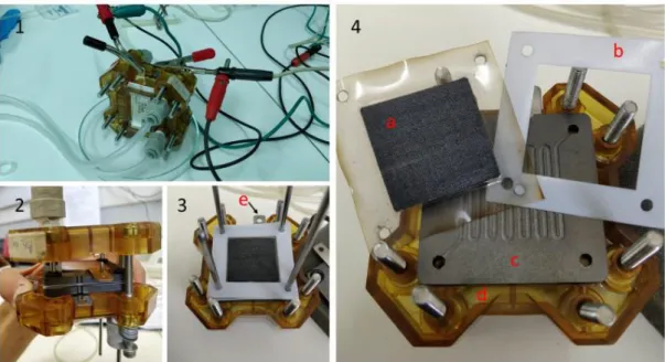
Figure 5 PEMFC. 1-Assembled fuel cell and connected to the circuit. 2/3/4- FC during assembly. a-Electrolyte membrane, b-Teflon gasket, c-Graphite Composite Plate, d-Molded plastic endplate, e-Nickel-coated brass current collector.

The circuit created to test the industrial hydrogen and biohydrogen is in the figure bellow.

Figure 6 Picture of the circuit created to test the biohydrogen. A-Parker TekStak Fuel Cell with graphite electrodes and platinum-rhodium electrolyte, B-Potentiometer, C-Voltmeter, D-Ammeter, E-Power source, F-Gas balloon, G-Air pump for gas, H-Air pump, I-Air washing bottle, J-Gas washing bottle, K-Water bath.

(23)

23

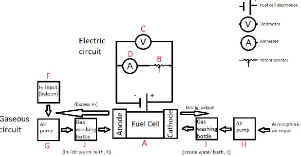
Figure 7 Schematic representation of the electric and gaseous circuit. A-Parker TekStak Fuel Cell with graphite electrodes and platinum-rhodium electrolyte, B-Potentiometer, C-Voltmeter, D-Ammeter, F-Gas balloon, G-Air pump for gas, H-Air pump, I-Air washing bottle, J-Gas washing bottle, K-Water bath.

3.2.2 Fuel Cell break-in

After the FC is assembled for the first time or after a long period of time, the next step is to activate the membrane in order to reach the best performance. This process is known as FC break-in. Before assembly the electrolyte membrane is dry and must be hydrated to maximize its ionic conductivity. For this first step, water at 50°C was forced in the H2

input (in the anode) to run through the circuit. At the same time, humidified and heated air, went in the cathode of the cell. For the second step the cell gets an input of heated and humidified H2 in the anode, and heated and humidified air in the cathode. This time the

point is to force an electrical current through the circuit to activate the catalysts in each electrode, forcing electrons to travel through from the anode to the cathode. This was done by applying a potential difference of 0.5V between the electrodes. After some minutes, the cell was ready to run and then the first test was done 27.

3.3 PEM Fuel Cell procedure

After assembly and break-in, the FC is connected in series with a potentiometer working as variable rheostat, an ammeter and a voltmeter in parallel (see figure 6 and 7). The gas balloon is connected to an air pump that regulates the flow according to the potential applied with the power supply, while assuring that no air goes back in the balloon. The gas travels inside a silicon tube until it reaches the gas washing bottle. This bottle is inside the water bath making sure the gas is humidified and heated at the desired temperature. At this point, the gas is ready to go in the cell. It goes through the internal circuit and the rest of the gas that did not react in the anode goes again to the gas washing bottle in a closed circuit. Because the minimum flow of the gas pump was much higher than the FC maximum consumption flow (approximately 60mL/h), the closed-circuit method was implemented to make sure the hydrogen from the balloon was enough for all trials. This way, at the beginning of each trial there was a continuous input of gas, with open circuit,

(24)

24 until the OCV was reached. After the circuit was fully saturated with biohydrogen, the tests began in closed circuit.

In parallel, for the air input, an air pump was used, forcing atmospheric air to go through another gas washing bottle to humidify and heat air at desired temperature into the fuel cell. The output for water vapour was open ended.

The experiment lasted while a continuous fermentation of food waste took place. It lasted 14.07 days and were produced 45.05 litres of gas composed mainly of H2 (around 98%).

The gas had also small amounts of oxygen and nitrogen, both inert for the fuel cell. During these days, 9 trials were made. Each trial at two different temperatures (25°C and 50°C). For each temperature, the sets were repeated between two and four times. For every analysis, a polarization curve was made from the values of current and voltage indicated in the ammeter and voltmeter. The same tests were made with industrial H2 in order to

(25)

25

4 Results and Analysis

4.1 Obtained data

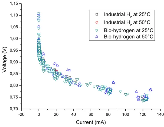
The Fuel Cell was fed with biohydrogen for 14.07 days, the same time that lasted the continuous fermentation of food waste. Along these days, 9 trials with biohydrogen were made, each one at 25°C and 50°C. The resulting biogas from DF was composed mainly of hydrogen (around 98%), nitrogen (around 2%) and traces of oxygen (around 1%). Both nitrogen and oxygen are inert for the FC membrane. In the next figure all the data collected during the full experiment is represented.

-20 0 20 40 60 80 100 120 140 0,70 0,75 0,80 0,85 0,90 0,95 1,00 1,05 1,10 1,15 Industrial H₂ at 25°C Industrial H₂ at 50°C Bio-hydrogen at 25°C Bio-hydrogen at 50°C Vo lta g e (V) Current (mA)

Figure 8 All obtained values of current and voltage throughout the whole study

All the values of biohydrogen at 25°C and 50°C, as well as the values with industrial hydrogen at both temperatures are represented in figure 8.

The resulting graphics and tables of all the individual trials are in the appendix chapter. As there was no clear difference in the power output at different temperatures, or between industrial H2 and biohydrogen, this section will focus on the trial that had the most energy

output (Test 8 at 50°C). The values of current and voltage of this trial are in the following table.

I(mA) V(V) I(mA) V(V) I(mA) V(V)

0,00 0,98 0,00 0,99 0,00 0,99

0,08 0,98 0,09 0,99 0,09 0,99

0,75 0,97 0,76 0,98 0,77 0,98

5,79 0,93 5,12 0,94 5,05 0,94

(26)

26

35,80 0,87 33,42 0,87 85,80 0,81

86,00 0,81 85,70 0,81 128,50 0,78

129,20 0,78 128,30 0,78

Table 1 Current and potential of 3 rehearsals with the same gas at 50°C

As the instruments used couldn’t set a fixed current, the results were analysed in OriginLab program to interpolate and find common points in the X axis as shown in the table below.

I(mA) V(V) I(mA) V(V) I(mA) V(V)

0 0,98 0 0,99 0 0,99 10 0,92 10 0,92 10 0,92 20 0,89 20 0,89 20 0,89 30 0,87 30 0,87 30 0,88 40 0,86 40 0,86 40 0,86 50 0,85 50 0,85 50 0,85 60 0,84 60 0,84 60 0,84 70 0,83 70 0,83 70 0,83 80 0,82 80 0,82 80 0,82 90 0,81 90 0,81 90 0,81 100 0,80 100 0,80 100 0,80 110 0,80 110 0,80 110 0,79 120 0,79 120 0,79 120 0,79

Table 2 Interpolated values of table 1

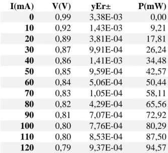
From the values of table 2, an average between the three rehearsals was made and this results in table 3. According to the equation (11), the power values were also calculated.

I(mA) V(V) yEr± P(mW) 0 0,99 3,38E-03 0,00 10 0,92 1,43E-03 9,21 20 0,89 3,81E-04 17,81 30 0,87 9,91E-04 26,24 40 0,86 1,41E-03 34,48 50 0,85 9,59E-04 42,57 60 0,84 5,06E-04 50,44 70 0,83 1,05E-04 58,11 80 0,82 4,29E-04 65,56 90 0,81 7,07E-04 72,92 100 0,80 7,76E-04 80,29 110 0,80 8,53E-04 87,50 120 0,79 9,37E-04 94,57

Table 3 Current, potential, standard error values and power measured in Test8_50

(27)

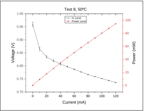
27 0 20 40 60 80 100 120 0.70 0.75 0.80 0.85 0.90 0.95 1.00 iV curve Power curve Current (mA) Voltag e ( V) 0 20 40 60 80 100 Power (mW) Test 8, 50ºC

Figure 9 iV curve of the average of interpolations in the same conditions of Test8_50.

In this case, there is no descending part of the power curve. The maximum power of this FC is the last point of the power curve. The voltage would reach zero and power would decline if the resistance was zero. And although the test resistance was as small as 4 ohm, there are also residual resistance of the cell itself and from the other devices connected in the circuit. This means that the zone of concentration losses was not reached, so the last point of the graph indicates the point with highest power.

In order to compare the performance of this FC with other studies, in figure 10 it is represented the same data of figure 9 but with values of current and power per cm2_.

0 2 4 6 8 10 12 0.70 0.75 0.80 0.85 0.90 0.95 1.00 iV Curve Power curve Current (mA/cm²) Voltag e ( V) 0 2 4 6 8 10 Power (m W/cm²)

(28)

28

4.2 Efficiency

In the point of the curve with highest power (Test8_50), the efficiency was 63%. Regarding all the trials, the efficiency values were always between 0.59 and 0.63. Being the average efficiency of the 25°C trials 0.598±0.006 and 50°C trials 0.601±0.007. For the control test with industrial hydrogen, the efficiency for both temperatures was 0.598. All these values are very close to each other (figure 11), and even if it was expected a higher efficiency for the 50°C trials, that was not observed.

Figure 11 Efficiency values for all trials, including control test with industrial hydrogen (10)

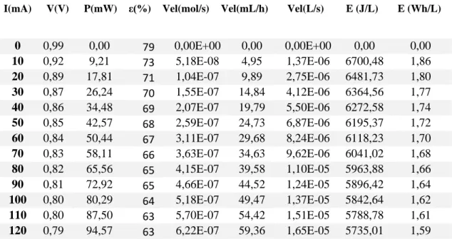
The equation (8) refers to the speed of H2 consumption (Vel) in mol/s. With this flow rate

it is possible to know how much of the gas was used in the cell. Using the ideal gas law, this rate may now be measured in L/s or mL/h. After all this logic, the energy generated calculation per litre of gas is now possible. All the results of the previous calculations are shown in the table below.

I(mA) V(V) P(mW) ε(%) Vel(mol/s) Vel(mL/h) Vel(L/s) E (J/L) E (Wh/L)

0 0,99 0,00 79 0,00E+00 0,00 0,00E+00 0,00 0,00 10 0,92 9,21 ₇₃ 5,18E-08 4,95 1,37E-06 6700,48 1,86 20 0,89 17,81 71 1,04E-07 9,89 2,75E-06 6481,73 1,80 30 0,87 26,24 ₇₀ 1,55E-07 14,84 4,12E-06 6364,56 1,77 40 0,86 34,48 ₆₉ 2,07E-07 19,79 5,50E-06 6272,58 1,74 50 0,85 42,57 68 2,59E-07 24,73 6,87E-06 6195,37 1,72 60 0,84 50,44 ₆₇ 3,11E-07 29,68 8,24E-06 6118,23 1,70 70 0,83 58,11 66 3,63E-07 34,63 9,62E-06 6041,02 1,68 80 0,82 65,56 ₆₅ 4,15E-07 39,58 1,10E-05 5963,88 1,66 90 0,81 72,92 ₆₅ 4,66E-07 44,52 1,24E-05 5896,42 1,64 100 0,80 80,29 64 5,18E-07 49,47 1,37E-05 5842,64 1,62 110 0,80 87,50 ₆₃ 5,70E-07 54,42 1,51E-05 5788,78 1,61 120 0,79 94,57 63 6,22E-07 59,36 1,65E-05 5735,01 1,59

(29)

29

4.2.2 Energy generated

The energy J/L in table 4, was calculated dividing the power (mW) by the consumption flow rate (mL/h), knowing that 1Wh is equivalent to 3600J. So, if 59.363mL were used in one hour, this fuel cell could deliver 5735 J/L. This means that during one hour at the actual consumption rate, 94.568mWh or 340.446 J are generated. These values correspond to the energy generated in the single cell FC used in this experiment. As the experiment lasted 337.68 hours (14.07 days), the total energy generated during the study with this specific fuel cell was 114.97 kJ (31.94Wh). The cell has an area of 10.89 cm2, so it produced a total of 8.68 mWh/cm2_{with an energy density of 11mA/cm}2_.

The FC used less fuel than the one available produced through dark fermentation. Knowing the flow rate of production, it is possible to calculate how big the FC needed to be to assure total consumption and electricity generation. The dark fermentation procedure lasted 14.07 days and 45.047 L of H2 were produced with a production flow

rate of 133.40 mL/h, and a consumption flow rate of 59.36 mL/h. This excess of flow could be totally used if the FC membrane was 2.25 times bigger. The power for this hypothetical case is in the next table, where power is calculated for 2.25 cells in case these values are needed for step up and further studies.

I(mA) V(V) P (mW) 0 0,99 0 10 0,92 248,29 20 0,89 240,19 30 0,87 235,84 40 0,86 232,44 50 0,85 229,58 60 0,84 226,72 70 0,83 223,86 80 0,82 221,00 90 0,81 218,50 100 0,80 216,50 110 0,80 214,51 120 0,79 212,52

Table 5 Power values for total generated fuel consumption

Considering the theoretical power output that the fuel cell would produce if it used all the fuel available (133.40 mL/h), it would generate 766 J (340.446J*2.25) in one hour, the same way it was calculated for the actual consumption of the fuel cell.

If all the fuel produced through the dark fermentation was used in a perfectly dimensioned fuel cell, with a biohydrogen production rate of 133.40mL/h, the energy generated would be 258.35 kJ (71.76Wh).

All the final results are summarized in table 6. Test8, 50°C Power output from FC (mW) Total Energy FC (Wh) Power output from DF (mW) Total Energy DF (Wh) Rate of generation (Wh/L) Rate of generatio n (J/L) 94,57 31.94 212.52 71,76 1.59 5735.01

(30)

30

Table 6 Final values of energy produced with FC rate and DF rate as well as the generation per litre of biogas.

The hydrogen percentage in the biogas was very high (approximately 98%). This resulted in very similar results between the industrial hydrogen and biohydrogen tests. For this reason, only the trial with the highest values of power and efficiency was studied (trial 8 at 50°C), in representation of all others. Also, the usual temperature of operation of a PEMFC is 50°C.

(31)

31

5 Conclusions and future recommendations

This thesis explored the integration of a fuel cell with biohydrogen produced from food waste fermentation. A total of 10 trials at 25°C and 10 at 50°C were made. In these experiments the temperature did not have significant influence in the FC performance neither the biohydrogen instead of industrial hydrogen.

The efficiency values (roughly 60% at maximum power) could be even higher than the ones obtained, one reason is due to the materials used. The FC is from 2006, the nickel coated current collectors showed a small amount of rust in its surface. The silicon tubes and connectors are not specialized for H2 transportation. The method of gas input in the

circuit could introduce traces of atmospheric air decreasing the efficiency as well. A reformulation of this study with specialized materials would give more accurate results, and probably higher values of efficiency and current.

Another future study would be studying the performance of biohydrogen in a FC with more than one cell and making another set of trials in order to have a full polarization curve, reaching the concentration overpotential for a better understanding of the behaviour of the system. Also, it is important to study the viability of DF sub products, such as fatty acids to produce electricity in microbial fuel cells and other products as land fertilizer.

(32)

32

6 References

1. Worldometers.info. Current World Population. Available at: https://www.worldometers.info/world-population/. (Accessed: 16th July 2019)

2. National Academy of Science. Population summit of the world’s scientific

academies. (1994).

3. Wackernagel, M., Kitzes, J., Moran, D., Goldfinger, S. & Thomas, M. The Ecological Footprint of cities and regions: Comparing resource availability with resource demand. Environ. Urban. 18, 103–112 (2006).

4. Stenmarck, Å. et al. Estimates of European food waste levels. Reducing food

waste through social innovation. Fusions (2016).

5. Hart, D., Lehner, F., Rose, R., Lewis, J. & Klippenstein, M. The Fuel Cell Industry

Review 2017. (2017).

6. Ballard Power Systems Inc. Ballard: Putting Fuel Cells to Work. Case Study -

Walmart Canada Fuel Cell Forklift Fleet 1 (2012).

7. Dincer, I. & Acar, C. Review and evaluation of hydrogen production methods for better sustainability. Int. J. Hydrogen Energy 40, 11094–11111 (2014).

8. Vincenzo Palma, Filomena Castaldo, P. C. and G. I. Sustainable Hydrogen Production by Catalytic Bio-Ethanol Steam Reforming. in Greenhouse Gases -

Capturing, Utilization and Reduction (ed. Liu, D. G.) 137–184 (2012).

9. Rahman, S. N. A. et al. Overview biohydrogen technologies and application in fuel cell technology. Renew. Sustain. Energy Rev. 66, 137–162 (2016).

10. Lin, C. N. et al. Integration of fermentative hydrogen process and fuel cell for on-line electricity generation. Int. J. Hydrogen Energy 32, 802–808 (2007).

11. García-Peña, E. I., Guerrero-Barajas, C., Ramirez, D. & Arriaga-Hurtado, L. G. Semi-continuous biohydrogen production as an approach to generate electricity.

Bioresour. Technol. 100, 6369–6377 (2009).

12. Wei, J., Liu, Z. T. & Zhang, X. Biohydrogen production from starch wastewater and application in fuel cell. Int. J. Hydrogen Energy 35, 2949–2952 (2010).

13. Andújar, J. M. & Segura, F. Fuel cells: History and updating. A walk along two centuries. Renew. Sustain. Energy Rev. 13, 2309–2322 (2009).

14. Falcão, D. Optimização de células de combustível com membrana permutadora de protões. (Faculdade de Engenharia da Universidade do Porto, 2010).

15. Nagamoto, H. Fuel Cells: Electrochemical Reactions. Encycl. Mater. Sci.

Technol. second edi, 3359–3367 (2004).

16. Shah, R. K. Introduction to fuel cells. Recent Trends Fuel Cell Sci. Technol. 1–9 (2007). doi:10.1007/978-0-387-68815-2_1

(33)

33 17. informationtrends.net. Close to 6,500 Hydrogen Fuel Cell Vehicles Have Been Sold Globally. (2018). Available at: https://www.altenergymag.com/story/2018/02/close-to-6500-hydrogen-fuel-cell-vehicles-have-been-sold-globally/27867/.

18. Jacoby, M. Fuel-cell cars finally drive off the lot. Chem. Eng. News 95, 29–32 (2017).

19. R. Zaetta, B. M. Hydrogen Fuel Cell Bus Technology State of the Art Review.

NextHyLights Version 3., (2013).

20. DANKO, P. Fuel Cells Power Up: Three Surprising Places Where Hydrogen Energy Is Working. National Geographic (2014). Available at: https://news.nationalgeographic.com/news/energy/2014/04/140403-fuel-cells-hydrogen-wal-mart-stationary/. (Accessed: 20th September 2007)

21. Ultra Electronics AMI fuel cells for UAVs, critical military tech. Fuel Cells Bull. 2013, 4 (2013).

22. Hodgson, S. Stationary fuel cells on a plateau. powerengineeringint.com (2017). Available at: https://www.powerengineeringint.com/articles/decentralized-energy/2017/12/stationary-fuel-cells-on-a-plateau.html. (Accessed: 20th September 2007)

23. Mansouri, I. & Calay, R. K. Sustainable hydrogen evaluation in logistics; SHEL.

Energy Procedia 29, 377–383 (2012).

24. Asst.prof. Dr. Hayder A. Dhahad1, Asst. Prof. Dr. Wissam H. Alawee2, E. A. E. S. Experimental Study Of The Operating Temperature Effect On The Performance of PEM Fuel Cell. World Res. Innov. Conv. Eng. Technol. 2016 (2016). doi:10.1007/s13127-011-0053-3

25. Imamura, D., Ebata, D., Hshimasa, Y., Akai, M. & Watanabe, S. Impact of Hydrogen Fuel Impurities on PEMFC Performance. SAE Tech. Pap. Ser. 1, 554–559 (2010).

26. O’Hayre, R. P. Fuel cells for electrochemical energy conversion. EPJ Web Conf. 148, (2017).

27. Parker. TekStak TM _INSTRUCTION _MANUAL _AND _REFERENCE

INFORMATION. (2006).

7 Appendix

In this chapter are presented the data for all the trials made during the FC operation. Tables of voltage and current of the several tests at different temperatures, tables of averaged interpolated and extrapolated values and respective graphics for each trial. Each trial was done in a day and consisted in several repetitions, each day at two different temperatures.

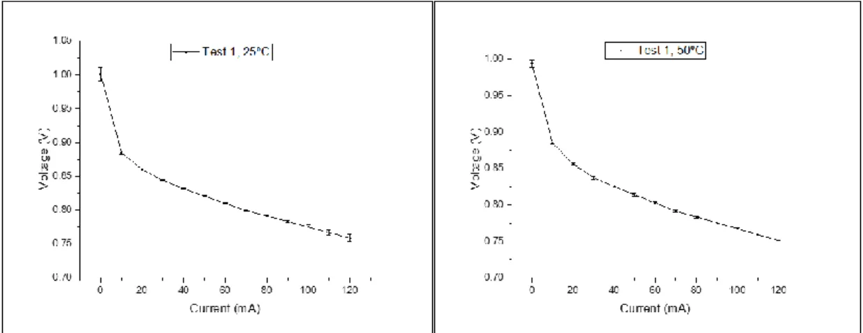
7.1 Trial 1, 16/out

(34)

34 0 0.987 0 1.021 0 0.994 0.08 0.987 0.01 1.018 0.01 0.993 0.21 0.986 0.09 1.016 0.09 0.991 0.8 0.966 0.4 1.008 0.8 0.97 1.01 0.96 0.81 0.975 1.96 0.946 2.04 0.938 1.05 0.957 4.7 0.914 4.82 0.91 1.81 0.941 11 0.884 6.55 0.901 2.81 0.927 24.07 0.854 9.49 0.888 3.63 0.913 44.82 0.827 13.42 0.875 5.13 0.9 73.7 0.797 17.14 0.866 11.4 0.874 76.6 0.795 24 0.852 24 0.848 43.55 0.827 59.27 0.81 72.8 0.796 74.1 0.795 75.2 0.796 76.1 0.794

Table 7 Obtained voltage and current data of Trial 1 at 25°C (3 repetitions)

I(mA) V(V) I(mA) V(V) 0 0.999 0 0.989 0.08 0.998 0.09 0.989 0.79 0.963 0.79 0.965 1.93 0.938 1.98 0.938 5.13 0.907 5.44 0.903 14.79 0.868 12.68 0.871 30.92 0.837 27.58 0.838 70.2 0.793 68.6 0.791 78.8 0.786 78.7 0.783

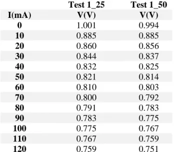
Test 1_25 Test 1_50 I(mA) V(V) V(V) 0 1.001 0.994 10 0.885 0.885 20 0.860 0.856 30 0.844 0.837 40 0.832 0.825 50 0.821 0.814 60 0.810 0.803 70 0.800 0.792 80 0.791 0.783 90 0.783 0.775 100 0.775 0.767 110 0.767 0.759 120 0.759 0.751

(35)

35

Figure 12 iV curves of averaged interpolated trial 1 values at each temperature

7.2 Trial 2, 19/out

I(mA) V(V) I(mA) V(V) I(mA) V(V) I(mA) V(V)

0 1.108 0 0.973 0 0.953 0 0.965 0 0.98 0.08 0.973 0.01 0.953 0.01 0.965 0.08 0.977 0.78 0.955 0.08 0.952 0.77 0.947 0.77 0.938 1.7 0.935 0.78 0.947 1.55 0.934 1.58 0.915 4.85 0.904 1.57 0.928 4.18 0.909 3.83 0.892 9.39 0.88 7.27 0.889 17.5 0.86 11.77 0.859 15.44 0.86 18.6 0.856 26.6 0.842 19.86 0.843 34.63 0.824 33.6 0.831 38.32 0.825 31.17 0.828 69.5 0.785 55.3 0.806 74.1 0.787 63.7 0.796 72.2 0.782 75 0.788 76.9 0.786 67.3 0.798 80.5 0.784 80.2 0.783 94 0.775 119.1 0.754

0 1.053 0 0.964 0 0.969 0 1.106 0 0.967 0.08 0.963 0.08 0.968 0 1.097 0 0.942 0.77 0.946 0.78 0.949 0.1 1.088 0.08 0.941 2.19 0.925 2.14 0.93 0.77 0.94 0.76 0.925 10.35 0.88 10.98 0.878 2.28 0.913 1.95 0.91 27.82 0.841 25.54 0.844 9.53 0.873 5.02 0.89 79.8 0.784 82.3 0.781 37.2 0.826 14.61 0.859 82.7 0.783 123.1 0.751 81 0.788 27.75 0.839 124.1 0.753 122 0.76 80.8 0.783 82.5 0.784 123.6 0.756

Test 2_25 Test2_50

(36)

36 0 0.984 1.005 10 0.878 0.878 20 0.851 0.855 30 0.834 0.838 40 0.821 0.826 50 0.810 0.816 60 0.800 0.806 70 0.792 0.795 80 0.786 0.785 90 0.782 0.778 100 0.777 0.771 110 0.772 0.764 120 0.767 0.757

Table 12 Average of interpolated values of trial 2 at each temperature

7.3 Trial 3, 23/out

0 1.08 0 0.957 0 0.964 0 0.962 0 0.922 0.08 0.956 0.08 0.963 0.08 0.96 0.08 0.92 0.76 0.941 0.77 0.949 0.76 0.941 0.73 0.908 1.65 0.928 1.86 0.931 2.02 0.924 2.03 0.893 4.28 0.902 5.51 0.898 11.94 0.872 6.98 0.865 14.2 0.86 17.92 0.853 29.49 0.835 19.19 0.838 37.61 0.82 33.43 0.825 72 0.787 69 0.786 71.3 0.785 71.5 0.784 102.5 0.765 71.3 0.787 100.4 0.762 99.9 0.763 -- -- 100 0.763 -- -- -- -- -- --

(37)

37 0.08 0.934 0.08 0.948 0.08 0.953 0.75 0.925 0.76 0.941 0.76 0.944 2.02 0.914 2.02 0.921 2 0.923 9.74 0.871 9.69 0.875 12.72 0.864 14.26 0.857 15.4 0.857 34.98 0.821 34.62 0.822 34.51 0.822 78.8 0.777 78.3 0.778 78.6 0.777 115.2 0.749 114.2 0.752 114.5 0.75

Test3_25 Test3_50 I(mA) V(V) V(V) 0 0.971 0.946 10 0.875 0.874 20 0.848 0.849 30 0.831 0.830 40 0.819 0.816 50 0.808 0.806 60 0.797 0.796 70 0.787 0.786 80 0.779 0.776 90 0.771 0.769 100 0.764 0.761 110 0.756 0.754 120 0.748 0.746

7.4 Trial 4, 24/out

(38)

38 0 0.943 0.08 0.963 0.09 0.967 0.08 0.941 0.77 0.955 0.77 0.956 0.75 0.922 4.23 0.909 4.59 0.908 2.23 0.903 14.69 0.864 18.12 0.856 10.62 0.864 56.05 0.801 42.6 0.814 31.7 0.826 82.8 0.776 82.4 0.774 83 0.777 124.8 0.743 124.4 0.742

0 0.942 0 0.957 0 0.959 0.08 0.942 0.08 0.957 0.08 0.959 0.75 0.931 0.76 0.945 0.75 0.943 5.07 0.89 4.89 0.9 4.97 0.896 18.13 0.846 19.65 0.845 17.17 0.848 32.32 0.822 46.3 0.804 42.17 0.807 82.4 0.77 81.6 0.77 81.4 0.768 124 0.739 122.3 0.739 122.1 0.737

Test 4_25 Test4_50 I(mA) V(V) V(V) 0 0.975 0.953 10 0.879 0.877 20 0.852 0.844 30 0.835 0.827 40 0.821 0.813 50 0.808 0.801 60 0.798 0.791 70 0.788 0.781 80 0.778 0.771 90 0.770 0.763 100 0.761 0.756 110 0.753 0.748 120 0.745 0.740

(39)

39

7.5 Trial 5, 25/oct

0 1.077 0 0.959 0 0.963 0 0.968 0 0.959 0.08 0.959 0.08 0.963 0.08 0.968 0 0.946 0.75 0.941 0.76 0.945 0.76 0.951 0 0.932 4.88 0.896 5.29 0.896 5.31 0.896 0.08 0.931 17.37 0.85 18.24 0.848 21.93 0.84 0.73 0.915 48.5 0.803 34.72 0.819 34.9 0.818 5.19 0.875 82.1 0.771 81.6 0.769 81.2 0.769 21.59 0.833 123.5 0.741 122.6 0.74 122 0.738 35.03 0.816 82.3 0.772 124 0.742 -- -- -- -- -- --

0 0.946 0 0.955 0 0.959 0.08 0.945 0.08 0.955 0.08 0.959 0.74 0.933 0.75 0.937 0.75 0.947 5.06 0.888 5.93 0.885 4.33 0.898 20.67 0.837 16.78 0.845 18.26 0.842 37.88 0.81 46.9 0.798 36.57 0.81 77 0.771 78.1 0.769 78.3 0.767 112.4 0.774 114.8 0.741 115.4 0.739

Test5_25 Test5_50

I(mA) V(V) V(V)

0 0.967 0.953

(40)

40 20 0.844 0.839 30 0.827 0.823 40 0.813 0.808 50 0.802 0.796 60 0.792 0.787 70 0.782 0.777 80 0.772 0.768 90 0.764 0.763 100 0.757 0.759 110 0.750 0.754 120 0.742 0.749

7.6 Trial 6, 26/out I(mA) V(V) I(mA) V(V) 0 1.093 0 0.958 0 0.929 0.08 0.958 0.08 0.927 0.75 0.945 0.72 0.911 5.1 0.897 5.47 0.868 21.37 0.843 19.58 0.832 41.37 0.814 31.65 0.819 82.2 0.774 82 0.775 123.8 0.745 123.2 0.745

I(mA) V(V) I(mA) V(V)

0 0.962 0 0.965

0.08 0.962 0.08 0.965 0.75 0.946 0.75 0.953

(41)

41 5.2 0.899 5.28 0.903 20.75 0.849 16.97 0.858 37.37 0.823 37.95 0.821 82.9 0.777 81 0.778 125.5 0.746 121 0.749

7.7 Trial 7, 29/oct

0 0.937 0 0.962 0 0.97 0 0.959

0.08 0.936 0.08 0.962 0.08 0.97 0.08 0.958 0.73 0.911 0.75 0.949 0.76 0.954 0.75 0.941 4.86 0.866 5.21 0.897 5.14 0.902 5.12 0.896

(42)

42 17.6 0.831 18.04 0.849 17.83 0.853 21.93 0.843

29.92 0.817 36.08 0.823 33.95 0.823 35.65 0.821 81.3 0.766 82.3 0.772 82 0.773 82.3 0.774 123.1 0.742 123.5 0.744 122.8 0.743 123.7 0.744

0 0.957 0 0.967 0 0.971 0.08 0.956 0.08 0.967 0.08 0.97 0.74 0.932 0.75 0.953 0.75 0.944 4.92 0.888 5.42 0.902 5.48 0.893 19.31 0.843 20.89 0.85 21.11 0.843 36.03 0.82 47.1 0.81 82.1 0.773 82.4 0.777 82.5 0.778 123.2 0.744 123.6 0.748 123.2 0.748

(43)

43 7.8 Trial 8, 30/oct

0 0.943 0 0.966 0 0.97 0.08 0.942 0.08 0.966 0.08 0.97 0.72 0.913 0.74 0.943 0.74 0.951 5.29 0.862 5.43 0.887 5.88 0.887 19.44 0.826 21.72 0.834 17.99 0.842 36.01 0.804 81 0.767 36.42 0.811 80.1 0.767 121.2 0.737 80.4 0.765 119.2 0.738 119.9 0.734

0 0.982 0 0.991 0 0.993 0.08 0.982 0.09 0.991 0.09 0.993 0.75 0.968 0.76 0.98 0.77 0.981 5.79 0.93 5.12 0.938 5.05 0.938 18.31 0.894 19.38 0.891 21.56 0.886 35.8 0.865 33.42 0.867 85.8 0.812 86 0.814 85.7 0.814 128.5 0.78 129.2 0.783 128.3 0.782

Test8_25 Test8_50 I(mA) V(V) V(V) 0 0.960 0.989 10 0.865 0.921 20 0.834 0.891 30 0.819 0.875 40 0.807 0.862 50 0.797 0.851 60 0.787 0.841 70 0.777 0.830 80 0.767 0.820 90 0.759 0.810 100 0.752 0.803 110 0.744 0.795 120 0.736 0.788