Gonçalo Vieira da Luz, nº 892
A Directed Research Project carried out under the supervision of: Professor Igor Cunha
January 2016
Leverage Instability and Persistence:
Evidence from the United States and Europe
2
Abstract
We find that leverage behavior both in level and time-series variation is very similar between the United States and Europe throughout the 1990-2013 period. Leverage regimes are simultaneously unstable and persistent for both regions. We define instability as the extent to which firms largely deviate from their long-term leverage mean, while persistence as the extent to which today’s leverage influences its future levels. We then show that this simultaneous evidence imply a mean-reversion behavior of leverage and discuss some of its implications for future research on this field.
The seminal work of Modigliani and Miller (1958) marked the beginning of the very active research field on corporate capital structures. Since then, all sort of theories have been proposed to explain the behavior of corporate leverage throughout time, especially in the United States. While many authors have been proposing broad theories supported by economic intuition to then test those with empirical data, others have chosen the reverse approach of empirically observing leverage behavior first, with an attempt to latter draw conclusions based on it. The work of Lemmon, Roberts, and Zender (2008, LRZ) on capital structure persistence, and the responsive work of DeAngelo and Roll (2015) both fall in the latter type. LRZ found empirical evidence in the United States for leverage persistence which, in their view, implies capital structure stability. DeAngelo and Roll later argued against such findings, by showing large within and across time-series variation of leverage, also in the United States.
The current paper presents an empirically and theoretically supported argument that reconciles the findings of both works, resorting to American and European data treated separately. We find that, in both regions, leverage is simultaneously persistent and unstable, which ultimately allows us to conclude that it also must be mean-reverting. The remainder of the paper is organized as follows: Section I presents the data and sample selection, Section II elaborates on the instability argument, Section III presents the persistence argument, Section IV reconciles both arguments, Section V explains the implications of all of the paper’s findings, and Section VI concludes.
3
I.
Data and Sample Selection
The sample of firms is taken from the WRDS-Factset Fundamentals Annual Fiscal (North America and International) database. It includes firms from the United States and 35 European countries for the 1990-2013 period. Financial firms (SIC codes 6000-6999) were excluded because capital structure in these firms is affected directly by the business model itself. Firms with a negative leverage ratio (total book debt divided by total book (or market) assets), leverage greater than 1 or non-available leverage information were also dropped. The initial sample includes 132.931 firm-year observations for the United States and 126.961 for Europe. After the adjustments we are left with 120.763 firm-year observations and 13.516 unique firms in the United States and 124.736 firm-year observations and 11.905 unique firms in Europe. All of the variables were winsorized at the top and bottom 1% level in order to smooth the impact of outliers. This is especially relevant for this study since firms after leveraged buyouts present temporary and non-representative abnormally high leverage values. Summary statistics and details on the variables used in the experiments can be found in the Appendix.
II.
Leverage Instability Within and Across Regions
We begin our analysis by examining and comparing the European and American leverage levels and their stability from 1990 to 2013. Hereafter, stability (instability) will denote the ability (inability) of a firm’s leverage ratio to remain within a strict band over a considerable period of time. Table I presents some statistics on market and book leverage for both regions. We split the firms in three different groups according to their number of years
4
available in the dataset in order to facilitate the comparison between regions and improve the robustness of the results. The first group comprises firms with less than 10 years of data, the second with more than 10 but less than 20, and the third group comprises firms with 20 or more years of data. Regarding leverage levels, we can observe in column (a) of each panel the median leverage for each group of firms. An interesting fact is that older firms present a larger median leverage ratio than firms with less than 20 years of data in both regions. This might occur since older firms tend to be larger, more established and more diversified, leading to a lower probability of default and bankruptcy costs as a proportion of firm’s value (J. Warner (1977), Ang, Chua and McConnell (1982) and Titman and Wessels (1998)). Another interesting result is that the median book leverage is very similar between regions for each group. For the first group, a median of 0,175 compares with 0,165 between the United States and Europe, for the second 0,158 compares with 0,165 and for the third 0,202 compares with 0,215, respectively. Despite the different institutional environment and the consequent potential for significant disparities, leverage ratios at the aggregate level are very similar during the period, something also noted by Rajan and Zingales (1995) across the G-7 for the 1987-1991 period. In terms of market leverage, the US presents a significantly larger leverage ratio for all groups of firms. This is explained by the greater overall equity market-to-book in this region, as can be noted in the summary statistics presented in the appendix. All of the results presented in terms of book leverage in the remainder of the paper were also computed for market leverage, with no relevant differences between them. Therefore, from here onwards, only book leverage analyses will be presented.1
To gauge whether European and American firms present stable leverage regimes and how do they compare, two different analyses consistent with the previous work done by DeAngelo and Roll (2015) were performed. The first one consists of determining the median
5
leverage range for each group of firms. To do so, we calculated the leverage range of each firm by subtracting the minimum leverage ratio (total book debt divided by total book assets) observed throughout its sample period from the maximum one. Finally, we computed the median of these set of ranges to arrive at the median range of leverage. This measure tells us how stable the leverage ratio of a representative firm within its group is. We can observe that the median range of book leverage implies non-trivial time series variation for all groups of firms, in both regions. The larger median range equals 0,351 and occurs in the United States for firms with more than 10 but less than 20 years of data. This is a remarkably large value specially when considering that the median leverage ratio for the same firms during the same period is 0,158, less than half of the corresponding range (0,351). And, again, the United States and Europe display very similar results. For the first group, a median range of 0,186 compares with 0,163 between the United States and Europe, for the second 0,351 compares with 0,294 and for the third 0,314 compares with 0,326, respectively. The median standard deviation was also computed to reinforce that the median range is a good proxy to measure leverage variability. Within each region, the greater the median range, the greater the median standard deviation. DeAngello and Roll also computed correlation coefficients very close to 1 between median standard deviation and median range for different groups of firms.
Another result worth noting is the fact that there is a large gap of median range between firms with less than 10 years of data and firms with more than that. Although a larger value would obviously emerge, since the latter firms had more time to vary, the fact that their range is almost the double may be an indication of the leverage speed of adjustment toward its mean. In other words, this may indicate that 10 years are not enough to explore the full range interval from which the mean (and potentially target) leverage ratio departs. Mean-reversion and leverage targeting will be further discussed in this paper.
6
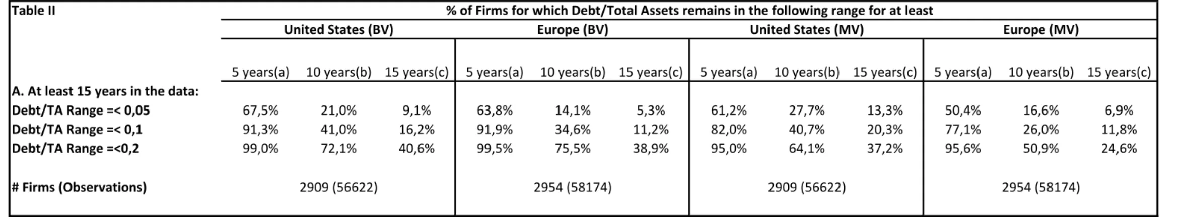
The second analysis was performed using only the firms with at least 15 years of data. This left us with a total of 2909 firms in the US and 2954 firms in Europe. In each row we can find the percentage of firms that remain in a particular leverage band for a particular number of consecutive years. For example, in the United States (Europe), among all the firms with more than 15 years in our sample, 67,5% (63,8%) of them managed to keep a leverage ratio within a band of 0,05 for at least 5 years. 21% (14,1%) did so for at least 10 years and only 9,1% (5,3%) for 15 years. We consider 3 definitions of a stable regime: one that does not fall out from a range of 0,05, another from a range of 0,1 and yet another from a range of 0,2. The number in the table reflecting greater stability is the one in the first row and column (c) of each panel, as it requires the firm to remain in the strictest band width (0,05) for the longest period of time (15 years). Only 9,1% of the firms in the United States are able to do so, while in Europe this number is as low as 5,3%. In this analysis there is a slight difference between both regions which indicates that leverage regimes are more stable in the United States than in Europe, with 16 out of the 18 directly comparable percentages being greater in the United States. However, the difference for the majority of them is not economically significant.
Again, the fact that most firms fail to remain in strict leverage bands for a decade or more reinforces the findings of Table I, i.e., that leverage regimes are unstable.
To summarize the current section, leverage ratios are very similar between the United States and Europe from 1990 to 2013 both in their median levels and variability. In both regions, statistical evidence points toward unstable leverage regimes over time in accordance with what has been previously found by Baranchuk and Xu (2008), DeAngelo and Roll (2015), and others. But are these findings really contradictory to capital structure persistence found by Lemmon, Roberts and Zender (2008) (LRZ hereafter), as DeAngelo and Roll defend?
7 Table II
5 years(a) 10 years(b) 15 years(c) 5 years(a) 10 years(b) 15 years(c) 5 years(a) 10 years(b) 15 years(c) 5 years(a) 10 years(b) 15 years(c) A. At least 15 years in the data:
Debt/TA Range =< 0,05 67,5% 21,0% 9,1% 63,8% 14,1% 5,3% 61,2% 27,7% 13,3% 50,4% 16,6% 6,9%
Debt/TA Range =< 0,1 91,3% 41,0% 16,2% 91,9% 34,6% 11,2% 82,0% 40,7% 20,3% 77,1% 26,0% 11,8%
Debt/TA Range =<0,2 99,0% 72,1% 40,6% 99,5% 75,5% 38,9% 95,0% 64,1% 37,2% 95,6% 50,9% 24,6%
# Firms (Observations)
% of Firms for which Debt/Total Assets remains in the following range for at least
United States (BV) Europe (BV) United States (MV) Europe (MV)
2909 (56622) 2954 (58174) 2909 (56622) 2954 (58174) Table I Median Leverage (a) Median Range (b) Median St. Dev (c) #Firms
(#Obs) (d) (a) (b) (c) (d) (a) (b) (c) (d) (a) (b) (c) (d)
Years on Compustat
20+ (3rd group) 0,202 0,314 0,106 1352 (30590) 0,215 0,326 0,093 1337 (31029) 0,156 0,367 0,104 1352 (30590) 0,239 0,4882 0,138 1337 (31029)
10-19 (2nd group) 0,158 0,351 0,111 3564 (49487) 0,165 0,294 0,092 4191 (57110) 0,095 0,344 0,109 3564 (49487) 0,170 0,3803 0,123 4191 (57110)
0-9 (1st group) 0,175 0,186 0,094 8600 (40686) 0,165 0,163 0,072 6377 (36597) 0,085 0,112 0,073 8600 (40686) 0,165 0,161 0,081 6377 (36597)
Median, Median Range and Standard Deviation of Leverage by Region
United States (Book Leverage) Europe (Book Leverage) United States (Market Leverage) Europe (Market Leverage)
Table I reports the Median, Median Range and Standard Deviation of both Book and Market Leverage for American and European firms. Firms were split into 3 groups according to the number of years available on Compustat for each firm. The bottom row refers to firms with less than 10 years, the middle row refers to firms with more than 10 but less than 20 and the top row refers to firms with 20 or more years. Book Leverage is defined as Book Value of Total Debt divided by Book Value of Assets, while Market Leverage is defined as Book Value of Total Debt divided by a proxy of Market Value of Assets equal to Book Value of Total Debt plus Equity Market Value. Column (a) presents the median leverage of the corresponding data on a panel data basis. Column (b) displays the median range of leverage, where range is defined as the difference between the maximum and the minimum leverage of each firm throughout its sample years. Therefore, the total sample of this median value will equal the number of firms available, not the total number of observations. For example, for US firms with more than 20 years in the data (Book Leverage), the value 0,202 is computed by first determining the leverage range of each firm and then computing the median of all the ranges across firms. Column (c) shows the median standard deviation of leverage within each firm. These values were computed with the same methodology described for median range but with standard deviations instead. Finally, column (d) summarizes the number of firms and observations that satisfy the corresponding criteria.
Table II displays the percentage of firms remaining within a leverage band of 0,05 (first row), 0,1 (second row) and 0,2 (third row) for a particular number of consecutive years (displayed in columns). Therefore, the strictest criteria is found in the first row, column (c) of each panel, as it requires the firm to remain in the strictest band for the most number of consecutive years. That is why this number (9,1% for United States Book Value of Leverage, for example) is the lowest within its panel.
8
III. Leverage Persistence Within and Across Regions
Before examining the results of the current section, it is of extreme importance to define leverage persistence and distinguish this concept from leverage stability. While stability requires a firm to keep a leverage ratio fairly constant over time, i.e., with a fairly constant mean and a standard deviation or leverage range close to zero, persistence only requires today’s leverage to influence future leverage to a large extent. This implies that a stable regime will necessarily be persistent, but a persistent regime may very well be unstable. Baranchuk and Xu (2008) addressed this view by running AR(1) models and concluding that the large auto-regressive coefficient indicates a persistent regime, but at the same time a large variance of the error term indicates instability in leverage.
In order to find how persistent leverage regimes are, we extended the work done by LRZ to European firms to compare the results with their American counterparties. These authors based their argument in favor of strong leverage persistence on the influence of the first observation of leverage (Initial Leverage hereafter) in future values of leverage. They did so by performing regression analysis and by finding the influence of firm fixed effects in a variance decomposition analysis.
Since previous literature shows evidence for adverse crowding-out effects in fixed effect models and propose using pooled OLS instead2, we ran 3 pooled OLS models for each region. One of the models will be denoted as “Full Specification” and the other two are restricted versions of it. The Full Specification is as follows:
𝐿𝑒𝑣𝑒𝑟𝑎𝑔𝑒𝑖𝑡 = 𝛼 + 𝛽1𝐿𝑖𝑡 −1+ 𝛽2𝐶𝑖𝑡 −1+ 𝛽3𝑃𝑖𝑡 −1+ 𝛽4𝑆𝑖𝑡 −1+ 𝛽5𝑀𝑖𝑡 −1+ 𝛽6𝐸𝑖𝑡 −1+ 𝛽7𝐼𝑖𝑡 −1+ 𝜆 + ℇ𝑖𝑡
9
where L denotes Initial Leverage and corresponds to the first non-missing value of leverage. The inclusion of this variable forces us to drop the first observation for each firm to avoid an identity at time zero. C denotes Collateral and equals net property, plant and equipment at time t divided by total assets at t. We expect firms with a greater proportion of tangible assets,
ceteris paribus, to have lower debt costs and, hence, be more levered. P denotes Profitability
and equals net income at time t divided by total assets at t. The expected sign of this variable is ambiguous as higher earnings might either allow the firm to finance most of its investments internally (Pecking Order Theory) or confer it a higher debt capacity by generating large enough earnings to benefit more from the tax shield and meet its debt payments (Trade-off Theory). S denotes Size and equals the natural logarithm of sales. A larger firm tends to be more transparent and better diversified, both contributing to a reduction in the cost of debt. M equals Assets’ Market-to-Book ratio and reflects the degree of growth opportunities of the firm. Since suboptimal investments pursued to expropriate wealth from bondholders is likely higher for firms in growing industries, we expect a negative sign in this variable’s coefficient3. E equals EBIT’s Volatility, which measures the riskiness of a firm’s ability to meet its interest obligations. The higher it is, the higher the direct and indirect costs of debt financing for the firm. I equals the industry median leverage, which is expected to influence positively each firm’s leverage for two reasons. The first is that firms within the industry tend to have similar leverage determinants. The second is that copycatting peers’ leverage ratio may be a shortcut to avoid accountability or individual blame to the capital structure’s decision makers at distressed times. It is also included to control for industry characteristics not captured by the remaining determinants. Finally, 𝜆 denotes a year fixed effect.
10 Table IV Variables Partial SS (% of model's PSS) F (P-Value) Partial SS (% of model's PSS) F (P-Value) Partial SS (% of model's PSS) F (P-Value) Partial SS (% of model's PSS) F (P-Value) Partial SS (% of model's PSS) F (P-Value) Partial SS (% of model's PSS) F (P-Value) Model 46,7 40,1 458,4 426,0 942,9 989,9 243,9 308,1 349,0 442,8 690,0 977,9 100% (0) 100% (0) 100% (0) 100% (0) 100% (0) 100% (0) Initial Leverage - - - - 484,5 14750,8 - - - - 335,4 13786,7 - - - - 51% (0) - - - - 49% (0) Industry Median - - 411,7 10714,0 182,5 5557,7 - - 105,0 3732,1 56,4 2318,1 - - 90% (0) 19% (0) - - 30% (0) 8% (0) Collateral 2,1 48,6 0,6 16,8 0,4 13,1 222,2 7577,9 107,4 3814,6 70,0 2875,6 4% (0) 0% (0) 0% (0 91% (0) 31% (0) 10% (0) Profitability 0,3 7,7 0,4 10,6 0,5 15,6 0,1 2,9 0,1 2,0 0,0 0,4 1% (0,006) 0% (0,001) 0% (0) 0% (0,090) 0% (15,6) 0% (0,538) Log(sales) 0,0 0,1 0,4 9,5 0,7 20,3 0,4 13,7 0,3 9,4 0,1 5,0 0% (0,802) 0% (0,002) 0% (0) 0% (0) 0% (0,002) 0% (0,025) Market-to-Book 0,0 0,2 0,0 0,1 0,0 0,1 0,0 1,2 0,0 0,6 0,0 0,2 0% (0,695) 0% (0,756) 0% (0,833) 0% (0,282) 0% (0,447) 0% (0,676) EBIT volatility 13,5 312,4 5,6 144,8 2,4 74,1 2,8 96,3 2,9 102,5 1,0 39,9 29% (0) 1% (0) 0% (0) 1% (0) 1% (0) 0% (0) Residual 3747,8 3336,1 2851,6 2621,2 2516,1 2175,1 Total 3794,5 3794,5 3794,5 2865,1 2865,1 2865,1 ANOVA
Model 1 Model 2 Full Specification Europe
United States
Model 1 Model 2 Full Specification
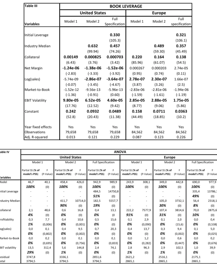
The regression’s and ANOVA’s outputs are summarized in Tables III and IV. Starting with Table III, the statistically significant coefficients are identified in bold and their corresponding t-statistics are between parentheses. The most notable fact about the pooled OLS results is the fact that adding the variables Industry Median and Initial Leverage to
Table III Variables Initial Leverage 0.330 0.321 (105.3) (106.1) Industry Median 0.632 0.457 0.489 0.357 (99.94) (74.26) (59.30) (45.49) Collateral 0.00149 0.000825 0.000703 0.220 0.164 0.138 (6.43) (3.76) (3.42) (85.96) (61.07) (54.5)
Net Margin -1.24e-06 -1.38e-06 -1.52e-06 0.000267 0.000203 2.74e-05
(-2.83) (-3.33) (-3.92) (0.95) (0.74) (0.11)
Log(sales) -5.74e-09 -2.86e-07 -3.64e-07 2.78e-07 2.30e-07 1.66e-07
(-0.07) (-3.45) (-4.67) (3.87) (3.26) (2.5)
Market-to-Book -1.52e-12 -9.56e-13 -5.96e-13 -2.83e-06 -2.81e-06 -1.94e-06
(-1.36) (-0.91) (0.60) (-1.59) (-1.61) (-1.19)
EBIT Volatility 9.80e-05 6.52e-05 4.60e-05 2.85e-05 2.88e-05 1.75e-05
(17.76) (12.52) (9.42) (8.77) (9.06) (5.86)
Constant 0.242 0.0932 0.0489 0.158 0.0711 0.0363
(52.8) (20.43) (11.38) (44.49) (18.85) (10.2)
Year fixed effects Yes Yes Yes Yes Yes Yes
Observations 79,658 79,658 79,658 84,562 84,562 84,562 Adj. R-squared 0.013 0.121 0.229 0.087 0.123 0.226 Model 2 Full specification Europe BOOK LEVERAGE United States
Model 1 Model 2 Full
11
Model 1 greatly improves the Adjusted R2. This is also true when we add Initial Leverage to Model 2, which reinforces the idea of leverage persistence. This is telling us that, even when we consider the main leverage determinants supported by capital structure theory, Initial
Leverage greatly boosts the explanatory power of our model by increasing the Adjusted R2 to near its double in both regions. Moreover, in the United States none of the variables besides
Industry Median and Initial Leverage have economic significance. In this region, for each
additional percentage point in Initial Leverage and Industry Median in the previous year, a firm is expected to have a leverage ratio 0,33 and 0,457 percentage points higher on average and holding everything else constant, respectively. In Europe, these marginal increments in leverage given an increase of 1 p.p. in each of the variables are equal to 0,321 and 0,357, respectively. LRZ obtained similar results for the United States, and clear similarities between regions can be observed once again.4 However, one more variable reveals to be both statistically and economically significant along these two in Europe. Collateral is the only economically significant variable in Model 1 and as we add Initial Leverage and Industry
Median to the regression, it still remains so. In the Full Specification, for each additional
percentage point of the lagged net fixed assets’ proportion to total assets (Collateral), a firm is expected to have a leverage ratio 0,138 p.p. higher. One institutional difference between the United States and Europe that might explain this disparity in the relevance of collateral is the relative importance of banks and financial markets in each country. Europe is a much more bank-oriented economy than the United States, when measuring this relevance by contrasting the amount of bank loans against bond and stock issues in both regions5. Since a bank loan only involves two parties, the lender in this case may reduce to a greater extent its exposure by stipulating specific conditions on collateral than it would be possible in a debt issue involving hundreds or thousands of lenders, each of them with its own taste. This might be
4
Although their reported values differ significantly since they present the standardized coefficients instead of their raw version as in here
12
one of the reasons why collateral seems to play such a prominent role in European capital structures compared to the United States.
Table IV presents an analysis-of-variance (ANOVA) for the same pooled OLS model. For each model we can find its partial (or explained) sum of squares, i.e., the portion of the total sum of squares explained by our independent variables, in the first row of each panel. Below the partial sum of squares of each variable we can find its corresponding portion in the model’s partial sum of squares. We calculate this percentage in order to gauge the relative explanatory power of each variable relative to the overall explanatory power of the model. Therefore, for the Full Specification Model in Europe, for example, the partial sum of squares of Initial Leverage represents 51% of our model’s explained sum of squares, which is found by dividing 484,5 by 942,9. We can observe that the explanatory power of every variable besides Initial Leverage and Industry Median is inexistent in the United States, along with what we have observed regarding economically significance in the pooled model. In the European case, Collateral has once again a significant role even after including Initial
Leverage and Industry Median. Most notable is the comparative relevance of Collateral
between the United States and Europe in Model 1, where it represents 91% of the explained sum of squares in the latter, but only 4% in the former. The partial sum of squares of the year fixed effects, the constant and the interaction terms were suppressed for simplicity purposes, and that is why the sum of the percentages in each column differs from 100%.
Overall, adding Initial Leverage to Model 2 improves the Adjusted R2 to almost its double and in both regions is by far the variable that contributes the most to the explained sum of squares. Considering this variable as a good proxy to measure capital structure persistence, we may conclude that leverage regimes are persistent in the United States and Europe, since that today’s leverage is the single most important determinant to future leverage.
13
One criticism made by DeAngello and Roll to the methodology used by LRZ was that, given the short-run stickiness in leverage, it is rather normal that Initial Leverage captures a large portion of the variation for firms listed just a few years. They argue that a narrow sample in terms of the average years of information for each firm would then inflate the R2 and overstate the explanatory power of Initial Leverage in ANOVA. But if this is the case, a higher Adjusted R2 should emerge from pooled regressions where the average number of years of information per firm is lower. This can easily be tested by progressively dropping the firms with the larger number of years and observe the behavior of the Adjusted R2. Table V presents the summarized results of running various pooled OLS regressions by successfully dropping from one to the next the firms with the most years of data in the panel. The first row corresponds to our previously presented Full Specification Model, since it includes all the firms with information within the 1990-2013 interval. The next row regards a model with the same variables, but using only firms with up to 22 years of information. The next one only regards firms with up to 20 years of information, and so on and so forth. We can see that the R2 of European firms does in fact progressively increase as we keep reducing the maximum years available for each firm in the sample, improving from 0,226 to 0,243, when the average years in the data goes from 10,5 to 8,0 respectively. However, the opposite happens in the United States, as dropping firms with more years of available information actually leads to a reduction in the Adjusted R2. When we run a pooled OLS with firms with a maximum of 16 years of available information, we end up with an average of 6,7 years per firm and the Adjusted R2 is 0,209, which compares to 0,229 when all firms were considered and the average number of years was 9. This indicates that short-run leverage stickiness and a biased sample toward firms with few years of data does not seem to be explaining the large influence of Initial Leverage found in LRZ and in this work.
14
Another criticism that can be made to LRZ’s graphical argument on leverage persistence is the way the portfolios are constructed each year. LRZ used a strong visual argument by providing an event year graph where the median leverage of four different groups split by leverage quartiles was plotted against time in the x-axis. The problem of their construction is that each year they rebalance the portfolio to calculate new leverage quartiles. They then average out the leverage quartiles of each event study to arrive at their final quartiles and average leverage for each of them. This approach tends to smooth quartile variation since low levered firms that leverage up their structure will offset the impact of high levered firms that deleverage their balance. By rebalancing the portfolio each year and allowing firms to migrate to another quartile, we are actually promoting leverage quartiles stability by construction, which is not desirable. To overcome this issue we performed an identical quartile analysis with the slight difference that the initial 4 portfolios split by leverage quartiles were kept intact except for extinguishment cases. Since the panel is unbalanced, we opted to perform an event study, meaning that the formation period of the 4 portfolios will include the first leverage observation for each of the firms comprising the sample. Therefore, the median leverage of our portfolios may very well cross each other at some point in time, as their composing firms are static and defined at period 0. Moreover, given the evidence in favor of non-trivial leverage instability, we would expect these portfolios to cross at some point in time if capital structures were not persistent.
Table V
Maximum years in the data per firm
Average years in the data per firm
# of firms # of observations
Adjusted R-Squared
Average years in the data per firm
# of firms # of observations Adjusted R-Squared 24 9,0 8850 79658 0,229 10,5 8053 84562 0,226 22 8,0 7791 62334 0,224 9,2 6934 63795 0,230 20 7,7 7530 57988 0,220 9,0 6687 60191 0,234 18 7,2 7018 50534 0,216 8,8 6433 56614 0,235 16 6,7 6302 42228 0,209 8,0 5764 46114 0,243
15 Graph I – Median leverage of American Portfolios
Graph II – Median leverage of European Portfolios
Graph I and Graph II display the median leverage of portfolios formed by sorting firms into quartiles according to their first observation of leverage, and keeping those portfolios unchanged throughout the period (except for extinguishment cases). Portfolios 2 and 3 present remarkable time-series persistence, while 1 and 4 display convergence toward intermediate portfolios. It is also important to note that low leverage firms and high leverage firms
0,00% 10,00% 20,00% 30,00% 40,00% 50,00% 60,00% 1 3 5 7 9 11 13 15 17 19 21 23 Portfolio Q1 Portfolio Q2 Portfolio Q3 Portfolio Q4 0,00% 5,00% 10,00% 15,00% 20,00% 25,00% 30,00% 35,00% 40,00% 45,00% 50,00% 1 3 5 7 9 11 13 15 17 19 21 23 Portfolio Q1 Portfolio Q2 Portfolio Q3 Portfolio Q4
16
(portfolios 1 and 4, respectively) remain so after 24 years of data, even though a clear convergence is present. This, again, reinforces the idea of persistence existent in capital structures in both regions and the similarities displayed between them.
To summarize this section, capital structure seems to be persistent both in the United States and Europe, with both regions presenting very similar pooled OLS and ANOVA factors for the variable Initial Leverage, used as a proxy for persistence. We also showed why the argument against this methodology given leverage short-run stickiness and biased small samples seems not to be true. Finally, a graphical argument was performed to reinforce the idea that leverage is persistent throughout time, by dividing the firms in each region in sticky portfolios and observing that each of them remained abnormally unchanged relative to the others. This allows us to answer the question that concluded the previous section: leverage regimes can be persistent even though they are unstable. But this leaves us with another puzzling question: what can explain these apparently contradictory characteristics to reconcile as they do?
IV. Mean-reversion in Leverage
The current paper and previous literature show that leverage is persistent, i.e., today’s leverage has a large explanatory effect in future’s leverage. It is also the case that capital structures are unstable, i.e., leverage ranges are wide during moderate periods of time when comparing them with the average leverage in those periods. But if leverage is persistent and it deviates significantly from its long-term mean from time to time, then it must be mean-reverting. The extent to what this long-term mean leverage is slowly moving or constant is another discussion and is out of the scope of this text. The important thing to note is that the argument holds in both situations. In fact, were the mean leverage to change widely across time, i.e., were the representative capital structure to display a strong trend, leverage could no
17 .2 5 .3 .3 5 .4 1990 1995 2000 2005 2010 2015 fyear
leverag, Winsorized fraction .01 meanid81
.2 5 .3 .3 5 .4 1990 1995 2000 2005 2010 2015 fyear
leverag, Winsorized fraction .01 meanid185
longer be persistent, as past leverage would have a weak explanatory power on current leverage.
To present this idea in a clearer form, we categorized leverage behavior regarding persistence and stability in 3 different types. The first type comprises firms with both stable and persistent regimes. The following line charts show how such regimes look like by depicting the evolution of leverage during 24 years (blue line) for 2 different American firms randomly chosen, as well as their long-term mean (red straight line):
Graph III Graph IV
Such regimes are stable, gauging by their leverage range across the period. The firm of Graph III has a range of 13,4% throughout the entire period and from 2002 to 2013 this range is lower than 10%. Considering that the mean leverage is 0,37, this regime can be considered very stable. It is also the case that leverage is very persistent in both firms. At each point in time, past leverage, even considering a very distant period, is a good predictor of current leverage. This must be the case as long as the regime is stable, since stability implies that leverage does not deviate too much from its long-term mean.
The second type of behavior includes firms that have leverage ratios that are unstable and non-persistent, as can be seen in the following graphs with the exact same axis and variables plotted as the previous ones, and also for two American firms:
18 0 .2 .4 .6 .8 1990 1995 2000 2005 2010 2015 fyear
leverag, Winsorized fraction .01 meanid49
0 .1 .2 .3 .4 1990 1995 2000 2005 2010 2015 fyear
leverag, Winsorized fraction .01 meanid470
.1 .2 .3 .4 .5 1990 1995 2000 2005 2010 2015 fyear
leverag, Winsorized fraction .01 meanid125
0 .1 .2 .3 .4 1990 1995 2000 2005 2010 2015 fyear
leverag, Winsorized fraction .01 meanid203
Graph V Graph VI
The firm in Graph V displays a range of 61% between 1900 and 2013, varying a lot between decades and presenting an unstable regime. Moreover, the firm starts with a low leverage ratio of 0,17 in 1990 and this ratio decreases to its sample minimum of 0,05 in 1992. From that year onwards, the ratio steadily increases with ups and downs until reaching its final value of 0,47. Graph VI depicts a leverage ratio with a smoother behavior throughout time, but still unstable, with a total leverage range of almost 40%, 20% for each 10 year sub-intervals and a long-term mean lower than that. What both firms have in common is a clear time-trend of leverage and, therefore, lack of persistence in their capital structures. In both cases, past leverage seems not to be a good predictor of current leverage and there is no mean-reverting behavior.
Finally, the third type of leverage behavior comprises firms that present unstable but at the same time persistent capital structures. The following graphs depict such behavior:
19
Both firms have leverage ranges close to 40% throughout the period, with the first having a long-term mean of 22% and the second 34%. Hence, during these 24 years of data, there is a large leverage variation around the mean. At the same time, current leverage is very close to the value observed 24 years ago, and this would be the case in most of the subintervals randomly chosen to compare leverage between two distant points in time. Most importantly, although leverage deviates considerably from its long-term mean, no trend in the ratio can be observed. Comparing Graphs VII and VIII with Graphs V and VI allows us to understand the underlying argument presented in this section: leverage regimes can only be persistent and unstable at the same time if the evolution of leverage does not display a clear time trend and, therefore, reverts to its mean after deviating from it.
So, we already found that leverage is simultaneously unstable and persistent and that the implication of this combination implies a mean-reverting behavior. But this still leaves us with the fundamental questions that have been puzzling researchers since the seminal work of Modigliani and Miller on capital structures: what is driving this mean-reversion behavior? Are managers aiming to a target leverage ratio? If yes, what are the factors taken into account upon determining such target? If no, is there any way the leverage ratio could be mean-reverting mechanically, i.e., with random financing and no targeting? These questions are conjectured in the last section of this paper to motivate future research on them.
V.
Active vs Passive Management of Capital Structures
Capital structure literature has been puzzling researchers since its theoretical foundations brought by Modigliani and Miller more than half a century ago. Since then, two things about this matter seem to be clear and prevalent throughout time. The first one is that progress on this field has been steadily increasing, with innovative ideas and methodologies developed to either bring new theories to the table or to empirically support past ones. The
20
second one is that, while effort and progress have been always present, no major conclusions have been achieved. It has always been a puzzle whether corporate managers target the level of debt with the purpose of maximizing the value of the firm, use leverage when it is more practical to do so or time equity issues when the stock is overvalued. It may also be the case that managers pursue any other strategy that is consistent with the various theories, that no one has thought about before or that involves no strategy at all.
One of the reasons why capital structure literature has been so controversial is precisely this plurality of drivers behind the decision. It will certainly be hard to prove empirically that the generality of firms target the leverage ratio to maximize the tax-shield, if only a portion of them do so, and perhaps not even always. It seems more sensible and rational to think that firms will end up pursuing a strategy that reconciles various theories. If it makes sense to issue debt up to non-dangerous levels to benefit from the tax-shield, or to repurchase equity if it is clearly undervalued, or even to fund real projects with internal funds to avoid transactional costs, most likely each firm will end up pursuing some or all of these actions throughout a long period of time. And if managers are actually managing leverage in accordance with various theories simultaneously, capital structure theories should not be approached as conflicting, as they have generally been. They should rather be viewed as complementary.
Another reason why it has been so difficult to support theories with unquestionable empirical evidence is that capital structure is affected by instruments whose usage can have purposes very different other than altering the leverage of the firm. Thinking about each and every factor that affects the ratio, an underlying business reason may be driving the shock in that factor. Equity issues decrease the leverage ratio and may occur either because the manager wants to deleverage the firm, because the firm needs funds to pursue a project, or even a mixture of both desires. If equity is issued with no funding needs, then the manager
21
must be aiming to create value through such an action. On the other hand, repurchasing its own stock might also be a desire to increase leverage or to return value to the shareholders, just as it is paying a dividend. Debt also has this dual facet, since it can be issued to finance real projects or to alter the firm’s capital structure. And to complicate things even further, basic business elements that represent the ultimate objective of current corporate organization, such as earnings and dividends, also impact capital structure over time. With all of these variables playing a significant role in the leverage of the firm, and considering that it is very hard to gauge what was the underlying intention behind a stock issue or repurchase, a debt issue, the retaining of earnings or a dividend payment, it is not difficult to understand why researchers have been having hard times reaching solid conclusions on this field.
Nevertheless, there is a distinction surrounding the way leverage emerges that is more easily addressed: active versus passive management of capital structures. It is important to note that each of them may comprise different theories. Therefore, showing empirically that capital structure is managed more actively than passively or vice-versa turns out to be a more feasible task than showing that a specific theory prevails. Active management will comprise all theories that support discretionary actions by managers that alter the capital structure of the firm, and whose underlying intention was not to fund a project or return value to the shareholder in a recurrent basis. These should include targeting and non-targeting behaviors such as the trade-off theory, where the firm is targeting an optimal ratio, or market timing, where the manager seeks for the best opportunities to create value to the existent shareholders either by repurchasing undervalued or selling overvalued stock. Note that the latter does not involve targeting a specific leverage ratio, but should fall under the active management theories since the manager is making use of capital structure’s instruments with the sole purpose of creating value to the shareholders, just as a tax-shield seeker does. Passive management should include Myers’ pecking order theory, where managers make use of debt
22
to finance projects when internal funds are not available and issue equity when their debt capacity is exhausted, or any other theories supporting inertia.
Some authors argue that mean-reversion is the continuous process of adjusting capital structure toward the target ratio (Shyam-Sunder and Myers 1999; Frank and Goyal 2003). However, Chen and Zhao (2005) argue that leverage ratios can revert to mean mechanically regardless of which theory better describes financing decisions, while Chang and Dasgupta (2007) show that mean-reversion may also be consistent with both the pecking order theory or even random financing. Hence, proving that leverage is mean-reverting may not be enough to conclude that managers are targeting the debt ratio.
So, how can we test if the generality of managers approach capital structure actively or passively? If capital structure management was purely passive, then the firms with the greatest capital expenditures throughout a period would be the ones issuing more equity and debt during that period, as that would be the only reason they would do such a thing. On the other hand, if capital structures are managed actively, the link between capital expenditures and equity or debt issues may not be that strong, since many firms with relatively few investment opportunities may be issuing securities to rebalance their structure. Hence, one way of getting a sense of how actively the firms are managing their leverage is to split a constant sample into quartiles of total capital expenditures, and then divide the same firms into quartiles of total equity and debt issues over the same period. If capital structure management is purely passive, we expect that the 25% of the firms falling into the first quartile of capital expenditures should also be the ones that mostly fall into the first quartile of securities’ issues. Only under such a scenario would we observe a corporate world in which issuing debt or equity had the main purpose of financing real projects, rather than creating value to the shareholders through indirect value enhancing mechanisms such as timing the market or creating a tax-shield.
23
Having this in mind, we built a constant composition sample within our dataset for all the firms remaining alive throughout the 1997-2011 period. This left us with 1940 firms in Europe and 1828 firms in the United States. We then split the firms into quartiles of total CAPEX during the period divided by total assets during the same period, leaving us with 4 groups of 485 firms in Europe (1940/4) and 457 firms in the US (1828/4). After this, we sorted the same firms into quartiles of total equity plus debt issues over the 15 year period, also standardized by assets so that each and every firm could be compared. We then looked into the firms falling into the first quartile of standardized CAPEX. These firms, being the ones with the lower investments pursued over the period, should also be the firms with the lower levels of issues, were capital structures to be passively managed. However, it turns out that in Europe 23% of them fall into the third quartile of total issues and 21% into the fourth quartile. This implies that 44% (23% + 21%) of the firms among the 485 needing the less in terms of funds are among the half issuing more debt and equity. This percentage amounts to 45% in the United States, where 20% of the firms falling into the first quartile of standardized CAPEX fall in the third quartile of standardized issues and 25% in the fourth. This represents a very large portion falling into the upper-end of debt and equity issues considering that around 100% of these firms should fall into the first quartile of such issues, if capital structures were passively managed (or, better said, not managed at all).
These figures, combined with the mean-reversion behavior previously observed, may indicate that firms are managing capital structures actively. However, it does not tell us the factors driving such behavior and the determinants behind the target. These, as stated before, will always be very hard to generalize given their complexity, diversity, and surrounding noise created by the intentions behind the usage of capital structure instruments.
24
VI. Conclusion
The debate on whether leverage is persistent or not has intensified in the later years with some authors arguing in favor of persistence and others against it. The current paper aims to demystify such debate by empirically testing leverage behavior in the United States and in Europe, while providing a clear view on what should be considered a persistent regime, as opposed to a stable one.
The major findings of this work are that time-series behavior of leverage is very identical between the United States and Europe, with both regions presenting simultaneously unstable and persistent regimes throughout the 24-year period considered. While instability was accessed through the large leverage range present in the average firm throughout the period, persistence was gauged through the economic importance of Initial Leverage in the determination of current leverage, both in pooled OLS and variance decomposition models. This combined instability and persistence leads us to conclude that the generality of firms must present a mean-reverse behavior of its leverage ratio. However, contrary to what has been once thought in the academia, this mean-reversion behavior is not a sufficient condition to infer that capital structures are actively managed, as shown by Chen and Zhao (2005) and Chang and Dasgupta (2007). For this reason, we end the paper computing a simple yet powerful exercise to show that leverage is probably actively managed, by showing that the firms with less funding needs are not necessarily the ones issuing less debt or equity.
These findings, along with the poor performance of the classical determinants thought to support the trade-off theory in our pooled OLS models, should constitute an incentive for future research on what might be driving this active targeting of leverage ratios in the United States and Europe.
25 References
Ang, James S., Jess H. Chua, and John J. McConnell, 1982, The Administrative Costs of Corporate Bankruptcy: A Note, Journal of Finance 37, 219-226.
Baker, Malcolm, and Jeffrey Wurgler, 2002, Market Timing and Capital Structure,
Journal of Finance 57, 1-32.
Baranchuk, Nina, and Yexiao Xu, 2008, On the Persistence of Capital Structure –
Reinterpreting What We Know, Working paper, School of Management of The University of Texas at Dallas.
Chen, Long, and Xinlei Zhao, 2005, Profitability, Mean Reversion of Leverage Ratios, and Capital Structure Choices, Working Paper, Michigan State University.
Dasgupta, Sudipto, and Xin Chang, 2009, Target Behavior and Financing: How Conclusive is the Evidence?, Journal of Finance 64, 1767-1796.
DeAngelo, Harry, and Richard Roll, 2015, How Stable Are Corporate Capital Structures?,
Journal of Finance 70, 373-418.
Flannery, Mark J., and Kasturi P. Rangan, 2006, Partial Adjustment Toward Target Capital Structures, Journal of Financial Economics 79, 469-506.
Gill, Balbinder Singh, Cross-country evidence on capital structure variability, Working paper, Vrije Universiteit van Brussel.
Graham, John R., and Campbell R. Harvey, 2001, The Theory and Practice of Corporate Finance: Evidence from the Field, Journal of Financial Economics 60, 187-243.
Lemmon, Michael L., Michael R. Roberts, and Jaime F. Zender, 2008, Back to the Beginning: Persistence and the Cross-Section of Corporate Capital Structure, Journal of
Finance 63, 1575-1608.
MacKay, Peter, and Gordon M. Phillips, 2002, Is There an Optimal Industry Capital Structure?, NBER Working paper No. 9032.
Mittoo, Usha R., and Franck Bancel, 2004, Cross-Country Determinants of Capital Structure Choice: A Survey of European Firms, Financial Management 33, No. 4. Modigliani, Franco, and Merton H. Miller, 1958, The Cost of Capital, Corporation Finance and the Theory of Investment, The American Review 48, 261-297.
Myers, Stewart C., 1984, Capital Structure Puzzle, Working paper, MIT.
Myers, Stewart C., and Lakshmi Shyam-Sunder, 1999, Testing Static Tradeoff Against Pecking Order Models of Capital Structure, Journal of Financial Economics 51, 219-244. Rajan, Raghuram G., and Luigi Zingales, 1995, What Do We Know about Capital
26
Structures? Some Evidence from International Data, Journal of Finance 50, 1421-1460. Titman, Sheridan, and Roberto Wessels, 1988, The Determinants of Capital Structure Choice, Journal of Finance 43, 1-19.
Warner, Jerold B., 1977, Bankruptcy Costs: Some Evidence, Journal of Finance 32, 337-347.