Background ozone over Canada and the United States

(1)

ACPD

9, 21111–21164, 2009

Background ozone over Canada and the

United States

E. Chan and R. J. Vet

Title Page

Abstract Introduction

Conclusions References

Tables Figures

◭ ◮

Back Close

Full Screen / Esc

Printer-friendly Version

Interactive Discussion

Atmos. Chem. Phys. Discuss., 9, 21111–21164, 2009 www.atmos-chem-phys-discuss.net/9/21111/2009/ © Author(s) 2009. This work is distributed under the Creative Commons Attribution 3.0 License.

Atmospheric Chemistry and Physics Discussions

This discussion paper is/has been under review for the journalAtmospheric Chemistry and Physics (ACP). Please refer to the corresponding final paper inACPif available.

Background ozone over Canada

and the United States

E. Chan and R. J. Vet

Air Quality Research Division, Science and Technology Branch, Environment Canada, 4905 Dufferin Street, Toronto, Ontario, M3H 5T4, Canada

Received: 24 August 2009 – Accepted: 21 September 2009 – Published: 7 October 2009

Correspondence to: E. Chan (elton.chan@ec.gc.ca)

(2)

ACPD

9, 21111–21164, 2009

United States

Title Page

Tables Figures

◭ ◮

Back Close

Full Screen / Esc

Abstract

Planetary boundary layer (PBL) ozone temporal variations were investigated on diur-nal, seasonal and decadal scales in various regions across Canada and the United States for the period 1997–2006. Background ozone is difficult to quantify and de-fine through observations. In light of the importance of its estimates for achievable

5

policy targets, evaluation of health impacts and relationship with climate, background ozone mixing ratios were estimated. Principal Component Analyses (PCA) were per-formed using 97 non-urban ozone sites for each season to define contiguous regions. Backward air parcel trajectories were used to systematically select thecleanest back-ground air cluster associated with the lowest May–September 95th percentile for each

10

site. Decadal ozone trends were estimated by season for each PCA-derived region using a generalized linear mixed model (GLMM).

Background ozone mixing ratios were variable geographically and seasonally. For example, the mixing ratios annually ranged from 21 to 38, and 23 to 38 ppb for the continental Eastern Canada and Eastern US. The Pacific and Atlantic coastal regions

15

typically had relatively low background levels ranging from 14 to 24, and 17 to 36 ppb, respectively. On the decadal scale, the direction and magnitude of trends are di_fferent in all seasons across the regions (−1.56 to +0.93 ppb/a). Trends increased in the Pacific region for all seasons. Background ozone decadal changes are shown to be masked by the much stronger regional signals in areas that have seen substantial

20

reductions of ozone precursors since the early 2000s.

1 Introduction

1.1 Ozone and air quality

Tropospheric ozone is an important component of photochemical smog which has seri-ous health e_ffects on humans (Burnett et al., 1996). The associated costs of health care

(3)

ACPD

9, 21111–21164, 2009

United States

Title Page

Tables Figures

◭ ◮

Back Close

Full Screen / Esc

and damage to vegetation can total up to billions of dollars annually in Canada alone (Canada, 2007). As tropospheric ozone is a secondary pollutant, its production and destruction processes are non-linear (Kleinman, l994; Klonecki and Levy, l997) which make the temporal and spatial variations in response to precursor emission changes difficult to understand. Ozone also regulates oxidation through the control of hydroxyl

5

radicals (OH), with OH being the dominant “cleansing” chemical in the atmosphere, an-nually removing gigatons of reactive trace gases and greenhouse gases (Ehhalt, 1999; Prinn, 2003).

1.2 Ozone and climate

As reported by the Intergovernmental Panel on Climate Change (IPCC, 2001, 2007),

10

tropospheric ozone is the third most important anthropogenic greenhouse gas (GHG), following CO2and CH4. IPCC studies have shown that tropospheric ozone is expected to continue rising (Ehhalt et al., 2001) due to the increase in economic activity of many developing countries as they consume more fossil fuel. In short, as the global tem-perature continues to rise, more favourable conditions for ozone formation will occur

15

(e.g., increased isoprene availability) (Zeng et al., 2008). Since tropospheric ozone is expected to have a direct positive radiative forcing on climate (Ehhalt et al., 2001; Ramaswamy et al., 2001), this continual positive feedback mechanism is projected to warm the earth’s atmosphere in the future. Modeling studies have shown that there is a strong inter-relationship between tropospheric ozone, GHGs, climate and regional air

20

quality (West et al., 2007; Fiore et al., 2008). Therefore, the quantification of di_fferent temporal variations of tropospheric ozone through observations is needed in current atmospheric research.

1.3 Background ozone

Background ozone may be considered as the portion of total surface ozone that results

25

(4)

ACPD

9, 21111–21164, 2009

United States

Title Page

Tables Figures

◭ ◮

Back Close

Full Screen / Esc

a given area. The mixing ratio of background ozone varies depending on geographic area, elevation, season, and averaging time (Altshuller and Lefohn, 1996). The term

backgroundis defined here as the planetary boundary layer (PBL) background (similar to what Fiore et al., 2003 defined) consisting of the combination of naturally and anthro-pogenically produced ozone from outside of Canada and the US, plus naturally formed

5

ozone within Canada and the US. The termbackground is hereafter to be understood as the Canadian and US background.

1.4 Temporal variations of tropospheric ozone

Ozone mixing ratios observed at remote locations are the result of ozone that is pro-duced and transported over long distances from upwind precursor sources

(anthro-10

pogenic and natural). Therefore, depending on the upwind locations of precursor sources, tropospheric ozone is expected to be heterogeneously distributed in time and space. Its atmospheric lifetime has been shown to be highly variable, from hours to weeks depending on time of the day, season and location (Schultz et al., 1999; Ehhalt et al., 2001; Fiore et al., 2002). Factors that control the lifetime of ozone are not

eas-15

ily separable (Wild, 2007). The observed long-term ozone trend at a given site, is therefore, expected to be obscured by the mixing of trends (possibly opposing) in the free troposphere (the hemispheric signal) and in the PBL (the regional and/or local signals). The magnitude and the direction of the long-term trends, especially for sec-ondary pollutants such as ozone are difficult to discern and explain most of the time

20

(Weatherhead et al., 1998; Jonson et al., 2006).

1.5 Air quality policy implications of background ozone

To further highlight the importance and quantification of background ozone, the follow-ing is a brief review of its implications on air quality policy. The air quality standard set by any jurisdiction must be attainable via domestic anthropogenic emission controls.

25

(5)

ACPD

9, 21111–21164, 2009

United States

Title Page

Tables Figures

◭ ◮

Back Close

Full Screen / Esc

Interactive Discussion controllable ozoneorpolicy relevant ozone(Fiore et al., 2002, 2003; Reid et al., 2008),

and refers to the amount that is possible to be controlled within one jurisdiction. By defi-nition then, the background of ozone cannot be reduced by precursor emission controls within Canada and the US. The magnitude of the effect of background has been shown in modelling studies to vary in di_fferent regions across the US (Fiore et al., 2002, 2003).

5

The estimated background in our study may be by various degrees influenced by re-gional anthropogenic sources (Altshuller, 1987; Altshuller and Lefohn, 1996). Thus, if the (continental and/or regional) background is indeed rising, the actual “controllable” amount by one local jurisdiction may become smaller in the future.

1.6 Previous research on background ozone

10

The quantitative values of background ozone in the PBL over the US have been esti-mated from both observations (Altshuller and Lefohn, 1996) and global chemical trans-port models (GEOS-Chem) (Fiore et al., 2002, 2003; Wang et al., 2009). Various pa-pers have shown significant increasingbackground ozone trend results in the Northern Hemisphere (Ja_ffe et al., 2007; Parrish et al., 2009, Chan, 2009) while other papers

15

have reported no significant changes (Oltmans et al., 2006, 2008). In Chan (2009), a multiple-site ensemble time series modelling technique was applied to characterize a decadal change in the ozone mixing ratios. This was done using di_fferent averag-ing metrics for the period 1997 to 2006 for many regions in Canada and the US. The evidence from that particular study showed that ozone trends decreased significantly

20

in southeastern Canada and the eastern US, whereas trends in coastal regions in-creased. No data screening was done to determine ozone mixing ratios associated solely with the background air.

1.7 Research questions

The foregoing research leads to a number of questions that are addressed in this

pa-25

(6)

ACPD

9, 21111–21164, 2009

United States

Title Page

Tables Figures

◭ ◮

Back Close

Full Screen / Esc

large areas of North America? Given the large intra-annual variations (noise) in ground level mixing ratios relative to the magnitude of the long-term trends (signal of interest), can the background ozone decadal trends still be reliably detected and, if so, what are they? How are the directions and magnitudes of such trends different in the four sea-sons in different regions of Canada and the US? Are the domestic precursor reduction

5

efforts in Canada and the US important for controlling regional-scale pollution in light of rising background ozone mixing ratios?

1.8 What is new in this study?

As mentioned above, it is difficult to define and quantify background ozone. Nonethe-less, there has been a tremendous amount of effort made in the past to identify and

10

separate different spatial (continental, regional, and local) and temporal (multi-year, seasonal, and diurnal) signals superimposed on each other. Backward trajectories have widely been used to classify air parcel transport using various statistical cluster-ing methods. Not limited to tropospheric ozone, a variety of atmospheric constituents have been investigated in the last few decades using trajectories (Dorling, 1992; Moody

15

et al., 1995; Pochanart et al., 2001; Vet et al., 2005; Bottenheim and Chan, 2006; Wor-thy et al., 2009, and many others). However, Parrish et al. (2009) have argued that continental e_ffects cannot be reliably eliminated by using large scale meteorological data such as air parcel trajectories. Undoubtedly, there is no universal method for all situations. The method introduced here is new in that it selects thecleanest or back-20

ground trajectory cluster which is associated with the lowest May–September 95th percentile of ozone (least amount of regional photochemically-formed ozone) for every measurement site. Consistent selection ofbackground air for all sites is demonstrated. As opposed to earlier work that provides an annual median background levels (Fiore et al., 2003; Vingarzan, 2004), here the diurnal and seasonal variations (cycles and

25

(7)

ACPD

9, 21111–21164, 2009

United States

Title Page

Tables Figures

◭ ◮

Back Close

Full Screen / Esc

the regional decadal trends of background ozone are estimated for the four seasons separately by region. The same statistical technique is applied throughout this paper to provide statistical consistency between the trend estimates of the various regions. This study provides a comprehensive analysis of background ozone variations in different chemical regimes over Canada and the US for the first time instead of focusing only on

5

the west coast as in previous studies (Jaffe et al., 2007; Oltmans et al., 2008; Parrish et al., 2009).

2 Data sources

The tropospheric, non-urban ozone data used in this study were obtained from the Canadian Air and Precipitation Monitoring Network (CAPMoN), the Canadian National

10

Air Pollution Surveillance Network (NAPS), and the United States Clean Air Status and Trends Network (CASTNET) of the US Environmental Protection Agency and National Park Service (NPS). In all, ninety-seven non-urban sites were used in the two countries, spanning latitudes from approximately 29◦N to 55◦N, and longitudes from 65◦W to 123◦W. The altitudes of the site locations ranged from 2 to 3178 metres above sea

15

level. Non-urban sites were used to minimize as much as possible local influences present in the data. Temperature observations, used to remove temperature e_ffects in decadal ozone trends, were obtained from the Canadian Climate Archive for ozone sites located in Canada and from on-site CASTNET temperature observations for sites in the US.

20

In the CAPMoN network, the sites are located in rural or remote areas and are con-sidered to be regionally representative. In the NAPS network, only the few sites located in rural locations were used, although, in general, they may have been more influenced by pollution from upwind urban areas than the sites in CAPMoN and CASTNET. Similar to CAPMoN, the CASTNET sites are rural in nature. Six-hour averages of hourly ozone

25

(8)

ACPD

9, 21111–21164, 2009

United States

Title Page

Tables Figures

◭ ◮

Back Close

Full Screen / Esc

emissions, nighttime scavenging and dry deposition, daytime averages (12:00–18:00 local standard time (LST)) were used for studying the decadal trends, i.e., the time when the PBL is fully developed and the air is expected to be well-mixed. Only sites with 75% or more data capture for every season for both ozone and temperature were used.

5

Three-day air parcel backward trajectories produced by the Canadian Meteorologi-cal Centre (CMC) were used to sort the six-hour-average ozone mixing ratios for this analysis. The trajectory calculations were made at that 925 hPa to avoid the influence of surface effects. At this level, the air flow is typically within the PBL (the mixed layer), well below the free troposphere and well above ground level. The CMC trajectory

10

calculations are based on the Canadian Meteorological Centre’s Global Environmen-tal Multiscale (GEM) model (C ˆot ´e et al., 2007). The trajectory calculations are not based on isentropic or isobaric assumptions. Trajectories calculated with the backward mean-trajectory model (BAM) show the 3-D displacement by mean wind vector at six-hour intervals. Trajectories were calculated for arrival times at the measurement sites

15

of 00:00, 06:00, 12:00, and 18:00 UTC every day.

3 Statistical method

3.1 Background ozone estimation

The method developed in this study uses the knowledge of ozone temporal behavior in response to regional photochemistry, combined with clustering of air parcel

trajec-20

tories, to objectively select the cleanest and most polluted air trajectory clusters for each site. Thecleanest clusters are assumed to representbackground air. The most-polluted clusters have been included here as a basis for comparing and contrasting the results of thecleanest clusters. Seasonal background levels and temporal varia-tions were calculated by fitting a one-year harmonic cycle to all six-hour-average data

25

(9)

ACPD

9, 21111–21164, 2009

United States

Title Page

Tables Figures

◭ ◮

Back Close

Full Screen / Esc

Eastern Canada, continental Eastern US, coastal/continental Western Canada, and coastal/continental Western US regions. Similarly, the diurnal background ozone lev-els and variations were estimated by fitting a 24-h cycle to all the hourly data associated with thecleanest air clusters for different seasons for a given region.

3.2 Seasonal principal component analysis

5

Principal Component Analysis (PCA) (SAS/STAT®, 1990) was done to identify ozone measurement sites that should be grouped together and thereby form different regions for the regional trend analysis that follows. The objective here was to use PCA to max-imize the total variance that could be accounted for by as few physically-meaningful regions as possible (Chan, 2009). PCA is a dimensionality reduction technique that

10

makes no attempt to form regions with equal numbers of sites. The regional group-ings were formed using the correlation matrix calculated from the six-hour-average ozone mixing ratios from the 97 non-urban CAPMoN, NAPS, CASTNET and NPS sites for the period 1997–2006 during the months of March-April-May (MAM), June-July-August (JJA), September-October-November (SON) and December-January-February

15

(DJF). Similar to Eder et al. (1993), varimax orthogonal rotation was used in this study. Seventy-five percent was the minimum total variance that had to be accounted for by the number of the underlying principal components in each season.

3.3 Backward air parcel trajectory clustering

A k-means clustering technique (Dorling et al., 1992) based on Euclidean distance was

20

used to sort the three-day air parcel backward trajectories from 1997 through 2006 into six trajectory clusters for each site. The method of determining the number of clusters (6) was the same as that used in Dorling et al. (1992). A graph was plotted for the total root mean square deviation (TRMSD) of all individual clusters from their cluster mean vector against the number of clusters retained. A jump in the TRMSD plot (not

25

(10)

ACPD

9, 21111–21164, 2009

United States

Title Page

Tables Figures

◭ ◮

Back Close

Full Screen / Esc

should be used. Six clusters were found to be common to most sites and were there-fore used throughout this study. In this context, trajectory clusters were considered to characterize the 10-year air flow climatology affecting the measurement sites.

With every six-hour trajectory at a site now being associated with one of six trajectory clusters, it was possible to bin the six-hour average ozone mixing ratio associated with

5

each trajectory to its appropriate trajectory cluster. Then, the 95th percentile ozone mixing ratio for May to September was calculated for every trajectory cluster. For each site, thecleanest background trajectory cluster was chosen as the one associated with the lowest 95th percentile of the six clusters. This cluster was assumed to represent background air flow with the least influence of regional/local-scale

photochemically-10

produced ozone, which generally contributes to peak levels in the summer. Thus, the least regional/local anthropogenic influences from Canadian and US emissions should be expected from these background clusters. For contrast, the opposite was also done to identify the most polluted trajectory cluster associated with the highest 95th percentile at each site.

15

3.4 Seasonal and diurnal variations using LOWESS

LOcally WEighted Scatter plot Smoothing (LOWESS) (Cleveland et al., 1988; SAS/STAT®, 1990) was used to display the seasonal and diurnal variations at each site in each PCA-derived region using the JJA-month groupings. The smoothing pa-rameter was chosen so that the periodicities of the temporal variations shown were

20

between a month and a year for the seasonal variations, and less than 24 h for the diurnal variations.

3.5 Regional decadal trends for di_fferent seasons

The robustness and the statistical significance of the decadal trends at individual sites are lower than desired because the data set comprised only the subset of data

cor-25

(11)

ACPD

9, 21111–21164, 2009

United States

Title Page

Tables Figures

◭ ◮

Back Close

Full Screen / Esc

and discern a decadal ozone trend for each PCA-derived region as a whole, a gen-eralized linear mixed model (GLMM) (SAS/STAT®, 2006), which serves as a multiple site ensemble technique, was used. The details of the time series model have been previously described in Chan (2009), but here it was run for each season separately.

In the time series model, the e_ffects of inter- and intra-annual variations due to

5

warmer versus colder weather were accounted for by using the daily maximum 1-h temperature as the covariate. The model also contained a one-day autoregressive term. Sine and cosine terms with three- to five-year periodicities were used to model the decadal trend component instead of a polynomial, which is often used. This was done to avoid collinearity with the linear slope term with respect to time. Neither

one-10

year nor six-month harmonic terms were included because the regional trend analyses were done for different seasons separately.

4 Results and discussion

4.1 Background ozone estimation

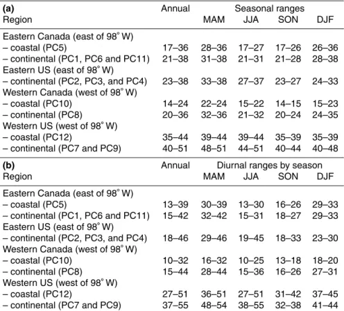
The quantitative estimates of seasonal background ozone are shown in Table 1a.

15

These represent the final calculations and are given here before showing the interme-diate steps that produced them. Using thecleanestdata sets to representbackground

ozone, the ranges (minimum and maximum) of the mean seasonal cycles shown in Table 1a were calculated using a least-squared fit with a one-year cycle to all the six-hour-average ozone mixing ratios associated with thecleanest background trajectory

20

clusters in a given region. This calculation was done for sites in coastal and continental areas of Eastern Canada, Eastern US, Western Canada and Western US separately. Background ozone levels varied seasonally in all regions. For example, the mixing ra-tios ranged from 31 to 38 in spring (28 to 38 in winter), and 33 to 38 (24 to 33) ppb for continental Eastern Canada and Eastern US, and, 22 to 24 (15 to 23) and 39 to

25

(12)

ACPD

9, 21111–21164, 2009

United States

Title Page

Tables Figures

◭ ◮

Back Close

Full Screen / Esc

These disparities in ranges are due to high elevations in the west compared to the east, and the close proximity to densely located ozone precursor emission sources for a large number of sites in the east. The values of the ranges for Canada are consider-ably lower than those for the US during the photochemically active seasons of spring (MAM), summer (JJA) and fall (SON). In coastal locations, the ranges are generally

5

lower than those in continental locations regardless of the season. Note that PC1, PC5, PC6, PC8, PC10 and PC11 (based on PCA-derived regions for JJA) show simi-lar seasonal variations and ranges with no apparent summer maxima which is typically associated with regional photochemically-produced ozone.

Similarly, as shown in Table 1b, the ranges of the mean diurnal cycles were

calcu-10

lated by fitting a 24-h cycle to all the hourly ozone mixing ratios associated with the

cleanest background clusters in a given region. This calculation was done for the four seasons separately. For instance, the results of the diurnal cycles of the ozone mixing ratios associated with thecleanest background clusters for coastal Eastern Canada estimated for the MAM, JJA, SON and DJF months ranged from 30 to 39, 13 to 30,

15

16 to 26 and 29 to 33 ppb, respectively. Serving as a diagnostic analysis tool, the amplitude of the diurnal cycle indicates the degree of local influence, with the wider the range, the greater the local influence (e.g., local precursor emissions). Generally, the ranges of the diurnal cycles are narrower for Canada than for the US during the photochemically active seasons, except for continental Western US where the ranges

20

were the narrowest.

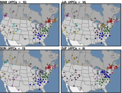
4.2 Seasonal principal component analysis

The varimax orthogonal rotation identified 13, 14, 11, and 8 PCA-derived regions for the MAM, JJA, SON, and DJF months, respectively. The PCA-derived regions (or principal components) were ordered by the percentage of the total variance explained

25

from the largest to the smallest. Sites that were grouped together had the largest loadings associated with that particular principal component.

(13)

ACPD

9, 21111–21164, 2009

United States

Title Page

Tables Figures

◭ ◮

Back Close

Full Screen / Esc

measurement sites. The large number of regions suggests that, as one would expect, major between-region di_fferences exist in emission source strengths and locations, air mass transport climatologies and atmospheric chemistry regimes. In general, from season to season the same regions exist with the exception of winter, in which there were fewer regions – indicating more spatial homogeneity than the other seasons.

5

The presence of the same regions from season to season suggests that all within-region sites share common air mass transport climatologies, precursor emissions and chemical reaction mechanisms. Figures 2, 3 and 4 support this.

Figure 2 shows, for each season, the 10-year-average backward trajectory (three day) at each site. It can be seen that the average air flow trajectories for all sites in

10

a given region have similar average flow directions. This implies that the precursor emission sources in the upwind direction are sufficiently similar for all sites in a given region.

This is further demonstrated by a Canadian chemical transport model, AURAMS (See Appendix), which was used to produce the seasonal domain-average mixing

ra-15

tio fields from the anthropogenic and natural emission sources of NOx and isoprene (Moran, 2009). The fields (Figs. 3 and 4) were produced from a 2002 AURAMS annual simulation base case run. NOx ambient mixing ratios do not vary substantially from season to season, but generally are higher in winter (DJF). Thus, only the NOxmixing ratio spatial distribution in JJA is shown. In contrast, the predicted isoprene mixing ratio

20

fields show four distinctively different spatial distributions. This is because the isoprene ambient mixing ratios are closely related to isoprene emissions from biogenic sources, which have strong seasonal variations caused by varying solar intensities throughout the year.

During the spring (MAM in Fig. 2), strong northwesterly flows predominate in the east

25

(14)

ACPD

9, 21111–21164, 2009

United States

Title Page

Tables Figures

◭ ◮

Back Close

Full Screen / Esc

suggests that, in general, the spatial distribution of precursor sources and their related emission strengths are more important than the transport patterns alone in terms of af-fecting ozone variability in this part of the continent. Indeed, the PCA-derived regions are largely similar to the high levels of the predicted NOxand isoprene ambient mixing ratio fields (Figs. 3 and 4). It appears that for example, the grouping of PC3

(Mis-5

sissippi, Alabama, Georgia and Carolina US) is the result of high upwind NOx mixing ratios from eastern US mixing with high regional isoprene from within the southeast-ern states. On the contrary, the grouping of PC8 (Alberta CA) may be due to regional NOxsources from within Alberta, Canada combining with high upwind isoprene mixing ratios originating in British Columbia, Canada.

10

In contrast, during the summer (JJA), the PCA-derived regions correspond roughly to the different mean transport patterns previously shown in Fig. 2. For instance, the short length and curvature of the mean trajectory paths in PC3 and PC4 (Illinois, In-diana and Ohio US) indicate a predominate stagnant air situation in the area. This recurring flow pattern in the east is attributed to clockwise air flow around the back

15

side of stagnant high pressure systems which transport polluted air masses northward (Lyons and Cole, 1976; Wolff et al., 1977; Wolffand Lioy, 1980). In addition, the two upwind high isoprene mixing ratio areas (dark brown, above 4 ppb) in the southeastern US (Louisiana, Arkansas and Missouri) appear to coincide with the mean flow direction for PC3 and PC4. For example, the groupings in the west appear to coincide roughly

20

with the regional NOx and high isoprene emission source areas in California. In gen-eral, the speed of the air flows is slower in the summer in most regions compared to other seasons indicated by the relatively short distance range of the backward trajec-tories.

During the fall (SON), the air flows are in transition from being predominately

slow-25

(15)

ACPD

9, 21111–21164, 2009

United States

Title Page

Tables Figures

◭ ◮

Back Close

Full Screen / Esc

NO_x sources, and northern Ontario and northern Quebec isoprene sources (possi-bly from Canadian boreal forests) contribute to the ozone variability of this particular PCA-derived region.

During the winter (DJF), the mean air flow directions are relatively homogeneous between and within regions and traverse over longer distances than in other seasons.

5

In other words, the meteorological influence is dominated by the continental wind flow pattern. Therefore, it is not surprising to see that the very narrow range of the diurnal variations (29–33 ppb, Table 1). This is partially the result of the wintertime longer-range and higher altitude transport that brings in clean background air, the low level of photochemical ozone production due to the reduced solar irradiance intensity, and

10

the much reduced regional/local isoprene mixing ratios (Fig. 4). In short, the winter PCA-derived regions do not compare directly with the spatial distributions of NOx and isoprene mixing ratios but fit well with the mean transport patterns.

4.3 Backward air parcel trajectory clustering

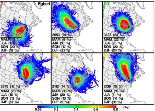
Egbert (44◦13′57′′N, 79◦46′53′′W), located in southwestern Ontario, Canada, was

se-15

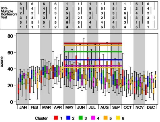
lected to illustrate the use of trajectory clustering to classify ozone data. First, six trajectory clusters were established (Fig. 5a) for this and every site. Then, each six-hour average ozone mixing ratio was allocated to its associated backward trajectory and binned into its appropriate trajectory cluster. In Fig. 5a, the cluster number (C1 to C6) is shown on the top left of each cluster panel and the relative transport frequencies,

20

in percentages for di_fferent seasons, are shown at the bottom left corner. For example, C1 represents the cluster of southwesterly flow trajectories and contains a total of 2471 (17%) trajectories over the period 1997–2006. Comparing across the six clusters for the same season, the transport frequencies attributed to this cluster are 15%, 17%, 20%, and 16% during spring (MAM), summer (JJA), fall (SON), and winter (DJF),

re-25

(16)

ACPD

9, 21111–21164, 2009

United States

Title Page

Tables Figures

◭ ◮

Back Close

Full Screen / Esc

and yellow horizontal bars, respectively. C6 was selected to represent the cleanest

background air for this site because the associated May–September 95th percentile mixing ratio is the lowest (yellow bar) compared to the other five clusters. The choice of this cluster as representing background air is further validated by this figure as it shows that a summer maximum, which is attributable to regional photochemically-produced

5

ozone, does not exist in C6. Additionally, the 5th percentile (lower whisker) value is the highest of the clusters in winter, suggesting that it is representative of continental background ozone because it has not undergone destruction processes typical of the clusters influenced by western and southern NOxemission areas.

Monthly 95% multiple Bonferroni test results are shown at the top of Fig. 5b where

10

the Bonferroni test is a conservative test used to control family-wise error with normally distributed data such as ozone. The order of the clusters is from the highest (at the top) to the lowest (at the bottom) monthly mean mixing ratios associated with the clusters. Vertical bars that overlap clusters indicate that there is no evidence of significant sta-tistical differences between those clusters; alternatively, clusters not joined by vertical

15

bars are considered to be statistically significantly different. For example, identified as thecleanestbackground cluster, C6, this northerly flow cluster tends to have the lowest monthly mean ozone mixing ratios during the summer months. However, the Cluster 6 mean is not significantly different from the C4 mean, where C4 is a shorter trans-port cluster that has more northerly and easterly components than C6. The Bonferroni

20

testing therefore clarifies that the background mixing ratios (significantly lower in sum-mer) are associated with predominantly northwesterly and/or northerly flow. Themost polluted cluster, C1, is often associated with the highest monthly mean ozone mixing ratios during May through October and the means are always significantly different from the other clusters in the warm months.

25

Note that the statistics that were used to select the background trajectory clusters were based on May to September ozone data while the trajectory clusters themselves corresponded to all months in the 1997 to 2006 period. Figure 6a and b shows the

(17)

repre-ACPD

9, 21111–21164, 2009

United States

Title Page

Tables Figures

◭ ◮

Back Close

Full Screen / Esc

sentative site in each region which was chosen as the site with the largest communality value associated with the respective principal component for the JJA months. Note that the larger the communality of a site in the principal component, the better the site is explained by the respective principal component and thus, the more representative it is of the region. In Fig. 6b, the trajectory clusters shown are the ones associated with the

5

highest May–September 95th percentile ozone mixing ratios of the six clusters at each site. These clusters represent themost polluted air flows affecting the sites in order to provide a contrast to thecleanest background air flows shown in Fig. 6a.

Generally, thecleanest orbackground air clusters (Fig. 6a) for non-coastal sites are associated with northerly Arctic flows whereas, for coastal sites, they are associated

10

with oceanic (Pacific or Atlantic) flows. For the most part, the background air trajectory clusters traverse areas with minimal regional anthropogenic precursor sources (see the predicted NOx mixing ratio spatial patterns in Fig. 3 and the population density map shown in the centre of Fig. 6a). Although less important for the non-urban sites used in this study, it is important to note that the background value for each site may be

15

affected by ozone removal processes such as dry deposition and NO scavenging. The existence of such removal processes were evaluated by selecting themost pollutedair clusters as discussed later in this section. Thebackground air cluster selection is also confirmed by the transport frequency statistics shown at the lower left corner of each trajectory probability density panel. The statistics show that relatively frequent air flows

20

are attributed to the spring (MAM) and winter (DJF) months. These are the months when background air is typically being transported at higher altitude and over longer distance in the northern mid-latitudes (Wang et al., 2003).

Figure 6b shows the most polluted clusters for the same 14 selected sites, one in each region. In fact, the areas of highest transport probability densities for these

clus-25

(18)

ACPD

9, 21111–21164, 2009

United States

Title Page

Tables Figures

◭ ◮

Back Close

Full Screen / Esc

DC corridor. In the west, themost polluted clusters of PC8 and PC12 coincide with high NOx mixing ratios in Southern Alberta/Canada and the west coast of California/US, respectively. In thismost polluted set of clusters, the transport distance is shorter and closer to the surface (see Fig. 7a and b for average transport height of the background and most polluted clusters). Focusing on regions least affected by mountainous

ter-5

rain, the average transport height of thecleanest set of clusters is consistently about one km higher than themost polluted set of clusters. As well, the transport frequency statistics for most sites show opposite flow characteristics to those of thebackground

air clusters, i.e., themost polluted set of clusters have relatively frequent air flows dur-ing the summer (JJA) and fall (SON) months, when photochemistry is at maximum,

10

compared to other seasons.

4.4 Seasonal variations

One of the questions posed in the Introduction was whether domestic ozone precur-sor emission reduction efforts might still be important in light of the documented (see Sect. 4.6) increase in background ozone. Evidence is provided in the following sections

15

to address this question.

Many studies in the past have discussed the seasonal variations of tropospheric ozone. Typical of ozone in the Northern Hemisphere is a spring maximum (Simmonds et al., 1997; Monks, 2000), formed partly from enhanced photochemistry in the spring-time after a winterspring-time accumulation of air pollutants (Penkett and Brice, 1986) and

20

partly from a downward flux of stratospheric ozone (Daniesen and Mohnen, 1977; Viezee et al., 1983). A second characteristic is a summertime maximum that occurs in regions strongly affected by the photochemical production of ozone due to precursor emissions (Singh et al., 1978; Logan, 1985).

To investigate whether these characteristics occur at the sites in this study, the

sea-25

(19)

homo-ACPD

9, 21111–21164, 2009

United States

Title Page

Tables Figures

◭ ◮

Back Close

Full Screen / Esc

geneity (or inhomogeneity) of the seasonality in background ozone. With reference to thecleanest air clusters in Fig. 8a, the high springtime ozone peak and the lack of high summertime values in all but regions, PC2, PC3 and PC4 suggest the lack of active lo-cal or regional photochemilo-cal ozone production (Goldstein et al., 2004), but rather the influence of long-range transport to the site with air descending either from the Pacific,

5

Arctic or Atlantic Oceans, as shown earlier. In contrast, precursor-source-influenced air in Canada and the US appears to be strong in PC2, PC3 and PC4 (eastern, south-eastern and Midwest US) because of the presence of high summertime values. Not surprisingly, this suggests that, even for these non-urban sites, the importance of the background diminishes for sites located very close to high density precursor sources

10

and in areas where the frequency of subsidence inversions is high (Fiore et al., 2002, 2003). In addition, because of the similarity of the within-region seasonal profiles and the narrow range of variabilities over such large spatial scales, the method developed here provides confidence that the selection of the background air is satisfactory with the minimal existence of any regional photochemical signals in most of the regions.

15

This evidence also suggests that the subset of background ozone mixing ratios teased out from the entire data set of non-urban sites is spatially consistent and continental (possibly hemispheric) in nature with the exception of regions PC2, PC3 and PC4. It is interesting to note that the values of the spring maxima for the sites at higher elevation (PC7 and PC9) are very comparable to those closer to sea level. However, the summer

20

minima of the seasonal cycles at the high elevation sites are, in general, not as low, possibly because of fewer removal processes taking place at high elevation.

By way of contrast, the seasonal variations associated with the most polluted

air trajectory clusters (Fig. 8b) show that most of the measurement sites have the incrementally-enhanced spring maximum and the broad summer maximum, both of

25

(20)

ACPD

9, 21111–21164, 2009

United States

Title Page

Tables Figures

◭ ◮

Back Close

Full Screen / Esc

regional/local processes have affected the local ozone mixing ratios.

4.5 Diurnal variations

Diurnal cycles, plotted by season and by region, allow one to investigate the relative intensity of local ozone influences including boundary layer dynamics, photochemical production and dry deposition. The inclusion of diurnal variations in the analysis helps

5

to evaluate the degree of local impacts that potentially exist in the extracted background ozone data.

Figure 9a and b shows the average diurnal cycles of ozone associated with the

cleanest and most polluted air clusters by season for each PCA-derived region, re-spectively. Diurnal variations that peak in the afternoon are influenced by the

com-10

bined effects of vertical entrainment of air from aloft by the growing convective PBL, the inflow of ozone due to transport from outside the location, and in-situ photochem-ical production. Nighttime and early morning decreases in mixing ratios are expected to occur more from surface destruction than from chemical scavenging because of the non-urban nature of the sites (i.e., distant from major NO sources) (Singh et al., 1978).

15

In this study, additional insights are gained from the large number of non-urban sites affected by minimal-to-high regional NOxand isoprene emission sources, and low and high elevation areas in Canada and the US.

In general the diurnal cycles associated with themost polluted air are about a factor of two higher than those associated with the cleanest air throughout the day during

20

the summer (JJA, red curves) and always lower during the winter (DJF, blue curves). The only exception to this is PC13, for which the nocturnal minimum associated with themost polluted air cluster is lower than that associated with the cleanest air clus-ter, although the daytime maximum associated with the most polluted air cluster is higher than that associated with the cleanest air cluster. This suggests that, at the

25

(21)

ACPD

9, 21111–21164, 2009

United States

Title Page

Tables Figures

◭ ◮

Back Close

Full Screen / Esc

dominates over other processes affecting ozone variability at non-urban sites. This pro-vides further confidence that the non-urban site selection in this study is appropriate for estimating background ozone levels.

Because the air parcel transport heights (Fig. 7a and b) are higher for thecleanest

clusters than for themost polluted clusters, thecleanest clusters are expected to have

5

more influence of downward entrainment of high elevation ozone. However, the diurnal cycles associated with themost polluted air are always of higher amplitude than those associated with thecleanest air in the daytime during the summer (JJA). This suggests that additional amounts of inflow ozone are transported to the sites from upwind pre-cursor sources, which dominates over the ozone that is vertically mixed down to the

10

surface during the day and is scavenged and/or surface deposited during the night. The mixing ratios associated with the diurnal cycle of PC9 for thecleanest clusters are the highest of all regions (Fig. 9a). Theoretically, without additional local photo-chemical production, the maximum diurnal mixing ratios in other regions should not exceed this upper limit of 50–55 ppb. Note that this upper limit is similar to the one

15

for Europe reported by Chevalier et al. (2007) of about 40–60 ppb above the top of the planetary boundary layer (at approximately 3 km). The evolution of the diurnal cycle should, for “pristine” sites at mid-latitudes (completely free of precursor sources), be the direct result of the development of the growing convective boundary layer and the mixing of high ozone upper air downward to the surface (Singh et al., 1978). For the

20

most part, this appears to be true for the ozone data associated with thecleanest back-ground air clusters. However, as shown in Fig. 9b, this upper limit remains more or less the same for themost polluted air flows in PC9, but the daytime ozone peaks in many regions do exceed this upper limit. This suggests that local photochemically-produced ozone does not exist in thecleanest background air clusters, but does exist in themost 25

polluted air clusters.

(22)

ACPD

9, 21111–21164, 2009

United States

Title Page

Tables Figures

◭ ◮

Back Close

Full Screen / Esc

a result, smaller diurnal variations should occur at the high elevation sites than at sites near or at sea level. This is indeed the case for PC9, the region that contains the highest elevation sites. Here, mixing ratios decrease only minimally at night (Fig. 9a) which, in turn, suggests that depositional and chemical losses are minimal at night. Similarly, the lack of a strong daytime maximum suggests that daytime production of

5

ozone from local precursors is minimal or, in other words, long range transport of non-locally-produced ozone is the dominant source of ozone at these high elevation sites.

4.6 Regional decadal trends for different seasons

The foregoing trajectory clustering technique allowed us to produce estimates of back-ground ozone in North America. The analysis was extended further to produce

es-10

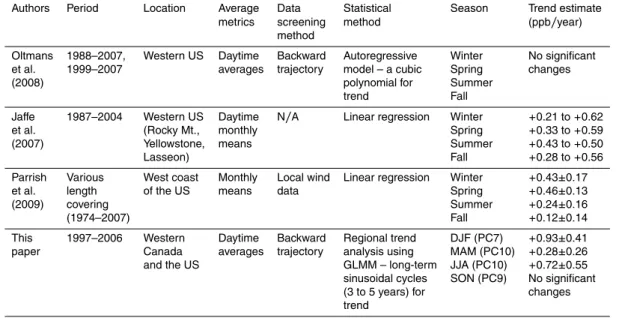
timates of the decadal trends of North American background ozone. To that end, decadal trends of daytime (12:00–18:00 LST) average ozone mixing ratios were mod-elled using the GLMM technique for the four seasons and for all PCA-derived regions. The results are shown in Table 2, for only the trend estimates that are statistically sig-nificant at the p<0.05 level. Figure 10 shows the trend results in map form with all

15

statistically significant trends being shown with a black line at the regional boundary. For comparison, Table 3 provides a tabulated summary of background ozone trends from three recently published papers that have investigated the trends of inflow air impacting the coastal areas of North America (Jaffe et al., 2007; Oltmans et al., 2008; Parrish et al., 2009). This paper uses a multi-site modelling approach to draw regionally

20

representative conclusion compared to single-site trend analysis in previous studies. It is important to note here that the direction of the decadal trends in Table 2 is more robust than the magnitude of the trends. This is because the estimated magnitude depends on many factors, including: 1) the statistical method chosen, 2) the model formulation and parameterization, 3) the representativeness of the rather small number

25

(23)

ACPD

9, 21111–21164, 2009

United States

Title Page

Tables Figures

◭ ◮

Back Close

Full Screen / Esc

in the data (tens of ppb from day to day). In light of the fact that such small amounts of data are associated with thecleanest background clusters, the multiple-site GLMM technique is advantageous compared to other techniques because it borrows statistical strength from the multiple site data. In other words, incorporating the between-site covariance within a region not only compensates for the potential problem of small

5

data sets but also improves the statistical power to detect small changes. The GLMM time series model and statistical details can be found in Chan (2009).

Temperature e_ffects were accounted for in the results shown in Table 2 and Fig. 10 by using daily 1-h maximum observation as the covariate in the time series model. In some regions, the temperature adjustment resulted in a switching of trend directions

10

but neither the unadjusted or adjusted trends were statistically significant. In general, the temperature adjustment tended to result in reductions in the magnitude of the sum-mer (JJA) trends only, with no systematic reduction or increase in the other seasons. This suggests that the temperature trend varied in the same direction as the ozone trend during the most photochemically active months. It is therefore, important that

15

the temperature effects be removed in the ozone variations in the summer, but not necessarily in the other seasons.

The results of the long-term trend analyses are not straightforward because the re-gions and the direction of the trends vary from season to season. The major results can be summarized as follows:

20

– In the Pacific coastal regions of southwestern British Columbia (Canada) and Cal-ifornia (US), the decadal trends were increasing in all seasons except fall (SON) in California. The trends were statistically significant in British Columbia in all seasons except the fall, but were not significant in California in any seasons.

– In the Atlantic coastal zone of southern New Brunswick and southern Nova Scotia

25

(24)

ACPD

9, 21111–21164, 2009

United States

Title Page

Tables Figures

◭ ◮

Back Close

Full Screen / Esc

spring.

– The eastern part of Canada and the US (i.e., east of Lake Superior in Canada and east of the Mississippi River in the US), showed negative trends in all regions in all seasons, with three exceptions: 1) the insignificant positive trends in Atlantic Canada/northeast Maine in the summer, fall and winter (discussed above), 2)

5

a significant positive trend in winter (DJF) at sites located in the US Midwest (Ohio, Indiana and Illinois), and 3) significant positive trends at all sites in Quebec (Canada) and one site in Vermont (US) during the summertime.

– At all sites all central/western Canada and the US, the trends tended to be nega-tive in the spring and fall but posinega-tive in the summer and winter. It is worth noting

10

however, that the density of the sites in the central and western regions was very low – meaning that the representativeness of the regions was considerably lower than for regions in the east.

Although the individual regional trends are difficult to interpret, collectively they ex-hibit similar tendencies over large areas of North America. For example, the Pacific and

15

Atlantic coastal regions of Canada and the US generally exhibit positive trends while the continental regions of central/western Canada and the US tend to exhibit nega-tive trends in the spring and fall and posinega-tive trends in the summer and winter. This is consistent with previously published studies at background and/or free troposphere sites that documented increasing trends in mixing ratios, particularly in the winter and

20

spring months, over the last two decades (Jaffe et al., 2003, 2007; Lelieveld et al., 2004; Jonson et al., 2006; Oltmans et al., 2006; Derwent et al., 2007; Parrish et al., 2009).

In contrast, the regions in the high NO_x and NMHC emission areas of eastern Canada and the eastern US (i.e., PC2, PC3 and PC4 in the SON map of Fig. 10)

25

(25)

ACPD

9, 21111–21164, 2009

United States

Title Page

Tables Figures

◭ ◮

Back Close

Full Screen / Esc

the period 2000 to 2007 (Canada–United States, 2008). This again implies that these regions are not continentally or hemispherically representative.

The explanation of background ozone trends is not simple. Possible reasons include rising NO_xemissions from developing nations and higher CO and NO_xemissions from large scale forest fires. The latter might be a plausible explanation for the positive ozone

5

trends found along the west coast (Fig. 10) in that biomass fires that burned a large area of Siberia in the summer of 2003 and were transported to the west coast of North America, were the largest in at least 10 years (Jaffe et al., 2004). This illustrates the point that because of the slowly-varying nature of the background, the importance of this signal can easily be masked by any major regional-scale ozone signals.

10

5 Summary and conclusions

This study provided a comprehensive analysis of decadal, seasonal and diurnal tem-poral variations of background ozone in different chemical regimes over Canada and the US for the first time. Background ozone mixing ratios for North America were esti-mated from measurements taken at 97 non-urban sites covering most of the landmass

15

of Canada and the US from 24◦N to 56◦N and 65◦W to 123◦W (with altitudes ranging from 2 to 3178 metres) for days with air mass trajectories from thecleanest of 6 trajec-tory clusters at every site. As expected from the literature, the seasonal background ozone variations in most of the regions (mainly in Canada) located away from the ma-jor precursor emission sources yielded a single spring maximum (Fig. 8a). The results

20

indicate that, as one would expect, a singlebackground ozone level cannot be defined for all of North America. Rather, background ozone, as defined here, varied geograph-ically and seasonally. As previously published by Parrish et al. (2009) and Ja_ffe et al. (2007), it was found that sites in coastal regions (coasts of the Pacific and Atlantic Oceans), background levels are predominantly influenced by flow offthe oceans, while

25

(26)

ACPD

9, 21111–21164, 2009

United States

Title Page

Tables Figures

◭ ◮

Back Close

Full Screen / Esc

Those continental areas of Canada having few anthropogenic precursor emission sources to the north of the measurement sites (e.g. PC11, i.e., northwestern Ontario, Canada) were found to have background levels considerably lower than in the con-tinental areas where large anthropogenic precursor emission sources do exist (e.g. PC4, i.e., Ohio River Valley, southeastern US). For example, the mixing ratios annually

5

ranged from 21 to 38, and 23 to 38 ppb for continental Eastern Canada (PC1, PC6, and PC11) and Eastern US (PC2, PC3 and PC4), respectively. The Pacific (coastal Western Canada, PC10) and Atlantic (coastal Eastern Canada, PC5) coastal regions typically had lower background levels, ranging from 14 to 24, and 17 to 36 ppb, re-spectively. The regional disparities of the background levels suggest that the term

10

background for the heavily source-a_ffected areas does not represent the same back-groundas for the coastal or low-pollution-impacted continental areas of North America. Sites that are in close proximity to high NOx and isoprene emission sources, even for non-urban sites, are shown to be impacted by regional pollution and are therefore not representative of the continental background.

15

Background ozone levels varied seasonally in all regions. For example, the mixing ratios ranged from 31 to 38 in MAM (28 to 38 in DJF), and 33 to 38 (24 to 33) ppb for continental Eastern Canada and Eastern US, and from 22 to 24 (15 to 23) and 39 to 44 (35 to 39) ppb for coastal Western Canada and coastal Western US, respectively. The background ozone estimates calculated in this study provides more detailed seasonal

20

and diurnal information for different regions compared to previously-published results and at the same time, these estimates fall within those published values for North America, ranging from 15 to 45 ppb (Trainer et al., 1993; Altshuller and Lefohn, 1996; Lin et al., 2000). Additionally, seasonal and diurnal cycles calculated from this study are consistent with those in other locations outside of North America (Logan, 1985;

25

Vingarzan, 2004; Oltmans et al., 2006), for example, in Greenland (Helmig et al., 2007), Ireland (Derwent et al., 2006), Japan (Pochanart et al., 2002), and China (Xu et al., 2008).

(27)

ACPD

9, 21111–21164, 2009

United States

Title Page

Tables Figures

◭ ◮

Back Close

Full Screen / Esc

trends decreased in most of the eastern US and eastern Canada in all seasons. For ex-ample, PC10 (Pacific Canada) had an increase of 0.28 ppb/a compared to PC2 (east-ern US) which had a decrease of 0.59 ppb/a. Note that this is a net decrease. Thus, the actual regional decrease might have been greater without the increase in back-ground. These results emphasize the important impact of regional and/or local ozone

5

precursor control efforts regardless of the slowly-varying (increasing) background. As shown in this observation-based study, the importance of background ozone appears to be offset in continental areas due to the large scale regional decrease of ozone in the planetary boundary layer through numerous ozone precursor emission reduction pro-grams over the last decade (Canada–United States, 2008; US EPA, 2007). However,

10

the relative importance of the background may increase in the future if the background continues to rise.

The main messages from this study are as follows:

– Increasing trends were observed along the Pacific coast of Canada and the US in all seasons, although the trends in California were not statistically

signif-15

icant. The statistically significant, temperature-adjusted ozone decadal trends in British Columbia, Canada increased at a rate of 0.28±0.26, 0.72±0.55, and 0.93±0.41 ppb/a in MAM, JJA, and DJF, respectively. If one assumes that the west coast increasing trends are representative of the hemispheric background, then it follows that, in the eastern US, the widespread decreasing trends

ob-20

served in all season must be due to regional ozone decreases caused by de-creases in ozone precursor emissions since the mid-2000s, e.g., the greatest decrease of the temperature-adjusted ozone trend among all eastern regions was−1.56±0.45 ppb/a (PC3 in JJA). This implies that our estimatedbackground

ozone levels for the eastern US are not truly representative of hemispheric

back-25

(28)

ACPD

9, 21111–21164, 2009

United States

Title Page

Tables Figures

◭ ◮

Back Close

Full Screen / Esc

– The similarity of the seasonal variations and the narrow ranges of variabilities over such large regions, particularly in the low pollution impacted regions of PC1, PC5, PC6, PC11, PC8 and PC10 as defined by PCA/JJA, the method developed here provides confidence in the selection of representative background air, with minimal influence of the any regional photochemical signals. This evidence also

5

suggests that the background ozone mixing ratios teased out from the entire non-urban data set are spatially consistent and continental (possibly hemispheric) in nature.

Appendix A 2002 simulation annual run using a CTM (Moran, 2009)

The ambient mixing ratios of NOx and isoprene were predicted using version 1.3.1 of 10

Environment Canada (EC)’s unified regional air quality modelling system (AURAMS) (Gong et al., 2006). The AURAMS AQ modelling system consists of three main com-ponents: (a) a prognostic meteorological model, GEM; (b) an emissions processing system, SMOKE; and (c) an o_ff-line regional chemical transport model (CTM), the AU-RAMS CTM. Each of these three components and the specific configurations chosen

15

for the 2002 annual simulation are briefly described in turn.

The Global Environmental Multiscale (GEM) meteorological model is an integrated weather forecasting and data assimilation system that was designed to meet Canada’s operational needs for both short- and medium-range weather forecasts (C ˆot ´e et al., 1998A,B; Mailhot et al., 2006). For the 2002 simulation, GEM version 3.2.0 with physics

20

version 4.2 was run on a variable-resolution North American regional horizontal grid. The grid consisted of a 353×415 horizontal global grid on a rotated latitude-longitude map projection. The grid spacing on the 270×353 uniform regional “core” grid was approximately 24 km (0.22◦), and the 28 vertical hybrid-coordinate levels reached from the Earth’s surface to 10 hPa. A model time step of 450 s was used.

25

(29)

ACPD

9, 21111–21164, 2009

United States

Title Page

Tables Figures

◭ ◮

Back Close

Full Screen / Esc

spatially disaggregated, and chemically speciated emissions for various CTMs from na-tional criteria-air-contaminant (CAC) emissions inventories (e.g., Houyoux et al., 2000; CEMPD, 2007). Version 2.2 of SMOKE (http://www.smoke-model.org/index.cfm) was used to prepare the very large set of day-specific emission files needed for the 2002 simulation. The three national anthropogenic emission inventories that were processed

5

by SMOKE to prepare input emission files for AURAMS were (a) the 2000 Canadian CAC emission inventory, (b) the 2001 US CAC emission inventory, and (c) the 1999 Mexican CAC emission inventory. Each of these inventories contained emissions of seven CAC species: SO2; NOx; CO; NH3; VOC; PM2.5; and PM10.

The AURAMS chemical transport model is a multi-pollutant, regional CTM that was

10

developed by EC as a tool to study the formation of PM, ozone, and acid deposition in a single “unified” framework. For the 2002 simulation, AURAMS version 1.3.1 was run on a 150 by 106 uniform, continental-scale North American regional horizontal grid on a secant polar-stereographic map projection true at 60◦N. The grid spacing was 42 km (Fig. 3). 28 vertical modified Gal-Chen levels reached from the Earth’s surface to

15

29 km. A model time step of 900 s was used, and AURAMS-predicted fields were output once an hour. Finally, the figures (Figs. 3 and 4) are the seasonal domain-average mixing ratio fields for the ambient mixing ratios of NOx and isoprene aggregated from the hourly outputs.

Acknowledgement. Thanks are due to Pierrette Blanchard (Environment Canada/Science

20

and Technology Branch, Toronto, Canada) for scientific advice, Michael Moran (Environment Canada/Science and Technology Branch, Toronto, Canada) for descriptions of AURAMS, Michael Shaw (Environment Canada/Science and Technology Branch, Toronto, Canada) for many SAS/GRAPH® software’s macros and subroutines, Jacinthe Racine (Environment Canada/Science and Technology Branch, Montreal, Canada) for performing numerous and

25

(30)

ACPD

9, 21111–21164, 2009

United States

Title Page

Tables Figures

◭ ◮

Back Close

Full Screen / Esc

References

Altshuller, A. P.: Estimation of the natural background of ozone present at surface rural loca-tions, J. Air Pollut. Control Assoc., 37, 1409–1417, 1987.

Altshuller, A. P. and Lefohn, A. S.: Background ozone in the planetary boundary layer over the United States, J. Air Waste Manage. Assoc., 46, 134–141, 1996.

5

Bottenheim, J. W. and Chan, E.: A trajectory study into the origin of spring time Arctic boundary layer ozone depletion, J. Geophys. Res., 111, D19 301, doi:10.1029/2006JD007055, 2006. Burnett, R. T., Brook, J. B., Yung, W. T., Dales, R. E., and Krewski, D.: Association between

ozone and hospitalization for respiratory diseases in 16 Canadian cities, Environ. Res., 72, 24–31, 1996.

10

Canada, Regulatory Framework for Air Emissions, Report on Canada’s New Government announces targets to tackle climate change and reduce air pollution, available online at http://www.ecoaction.gc.ca/, 2007.

Canada–United States, Canada-United States Air Quality Agreement-Progress Report 2008, available online at: http://www.ec.gc.ca/cleanair-airpur/caol/canus/report/2008CanUs/eng/

15

tdm-toc eng.cfm, 2008.

Canadian Council of Ministers of the Environment (CCME): Guidance Document on Achieve-ment Determination, Canada-wide Standards for Particulate Matter and Ozone, CCME Re-port PN 1391, available online at http://www.ccme.ca/assets/pdf/1391 gdad e.pdf, 2007. Chan, E.: Regional ground-level ozone trends in the context of meteorological influence across

20

Canada and the Eastern United States using a mixed model from 1997 to 2006, J. Geophys. Res., 114, D05301, doi:10.1029/2008JD010090, 2009.

CEMPD Center for Environmental Modeling for Policy Development SMOKE website, Uni-versity of North Carolina at Chapel Hill, North Carolina, USA, available online at: http: //www.smoke-model.org/index.cfm, 2007.

25

Chevalier, A., Gheusi, F., Delmas, R., Ord ´o ˜nez, C., Sarrat, C., Zbinden, R., Thouret, V., Athier, G., and Cousin, J.-M.: Influence of altitude on ozone levels and variability in the lower troposphere: a ground-based study for western Europe over the period 2001–2004, Atmos. Chem. Phys., 7, 4311–4326, 2007, http://www.atmos-chem-phys.net/7/4311/2007/. Cleveland, W. S., Devlin, S. J., and Grosse, E.: Regression by local fitting, J. Econometrics, 37,

30

87–114, 1988.