An endogenous business cycle model : theory and simulation

(1)

M

ASTER OF

S

CIENCE IN

M

ONETARY AND

F

INANCIAL

E

CONOMICS

M

ASTERS

F

INAL

W

ORK

D

ISSERTATION

A

N

E

NDOGENOUS

B

USINESS

C

YCLE

M

ODEL

:

T

HEORY AND

S

IMULATION

F

RANCISCO

O’N

EILL

C

ORTES

(2)

M

ASTER OF

S

CIENCE IN

M

ONETARY AND

F

INANCIAL

E

CONOMICS

M

ASTERS

F

INAL

W

ORK

D

ISSERTATION

A

N

E

NDOGENOUS

B

USINESS

C

YCLE

M

ODEL

:

T

HEORY AND

S

IMULATION

F

RANCISCO

O’N

EILL

C

ORTES

SUPERVISOR:

P

EDRO

A

LEXANDRE

R

EIS

C

ARVALHO

L

EÃO

(3)

Abstract

This dissertation has as its main objectives, taking the models for endogenous business cycles existing in the literature, firstly to build a new model and secondly to determine its actual capability to generate cycles and how different parameter values can change the results. The base model used was the capacity utilization model by Leão (2016), complemented with the profit squeeze model by Sherman (1991).

After we had run simulations using, as much as possible, plausible values for the parameters, it was found that the model can indeed generate business cycles that satisfy most stylized facts and whose shape depends on the parameters. However, the next step of estimating the parameters of the model for concrete real world situations remains still to be done.

Overall, our results suggest that the response of investment to deviations of capacity utilization from its desirable level, which is the main mechanism on which the model is based, plays a significant role in the explanation of how business cycles develop in real economies.

Keywords

business cycle, endogenous business cycle, simulation, capacity utilization, paradox of investment, reserve army, underconsumption, overinvestment

(4)

Acknowledgements

First of all, I would like to thank my supervisor, professor Pedro Leão, for the invaluable support in all phases of the building process of this dissertation: from the selection of the subject to the final writing process.

I also thank my brother João for introducing me to the software Wolfram Mathematica, which was a crucial tool to perform the simulations in which the main contribution of this work consists.

(5)

1. Introduction

The explanation of business cycles is a heavily studied problem in Economics, around which a great controversy has developed. In fact, there are a great number of competing theories that try to shed light on the mechanisms that cause economic variables to fluctuate overtime, from those that do not recognize business cycles as inherent to the economy, claiming that they are a result of external shocks, to those that try to explain endogenous mechanisms responsible for the permanent state of oscillation common to all capitalist economies.

Focusing in the latter view, in this work it is our aim to summarize the main existing theories and models and, taking their most important ideas, build a new model in which these complementary but often isolated theories are allowed to coexist. It is naturally expected that the joining of well supported complementary ideas in the same model will enhance its overall explanatory power.

In a next step, using simulations, we will analyze the results that the model can generate and confront them with observed characteristics of business cycles. This will be our main contribution, in the sense that, while the mechanisms on which many business cycle models rely have been quite well discussed in the literature, the evaluation of the same models considering the results that they can numerically generate is still incipient for most of them. In fact, even after understanding all the mechanics of the models, it is not an easy task to figure out what the result will be and how the values of the parameters can affect it. The analysis of the generated numerical results allows for a much more intuitive and at the same time more productive evaluation of the explanatory power of the model and its underlying mechanisms.

(7)

2

2. Overview of the main theories of the business cycle

There are in the literature many theories that explore financial conditions as determinants of business cycles, such as in Minsky (1982). While recognizing their importance, our approach will be focused from the onset on the real side of the economy.

2.1. Exogenous versus endogenous theories

When studying business cycle theory, there is an important classification to have in mind: that between endogenous and exogenous business cycle theories.

Exogenous theories explain the observed oscillations of output as a result of external shocks to the economy, which can be anything from a technological change to an increase in government spending. In fact, these theories assume that the economy, if there are no external shocks, grows smoothly and without oscillations along a long-run equilibrium position.

In turn, according to endogenous theories each phase of the business cycle has in itself the seeds that will start the next, and so cycles are explained without having to rely on external shocks to the economy (these can change the oscillations, but they are not needed for a cyclic behavior to occur). In this sense, endogenous theories can be called true or complete, because they are sufficient to explain their object of study. For this reason, we focus only on endogenous business cycle theories as the base on which we will build this work.

2.2. Investment as the key to business cycle theory

Because business cycles are defined as oscillations in aggregate income, the first step to study them should be to disaggregate this income into its constitutive parts. In a closed economy without government, demand can be divided into consumption and investment. Investment is in practice much more volatile than consumption, so it is natural that most theories give it an important role in explaining the cycles, which are all about volatility. In fact,

(8)

3 for more than a century, investment has been widely accepted as the key variable explaining business cycles. In most business cycle theories, there is a two-way relationship between investment and the economic situation. An overview of the way in which this mechanism can take place is provided in what follows.

2.2.1. How investment affects output

The mechanism through which investment affects output can be understood with the simple Keynesian multiplier. As mentioned above, in a closed economy without government, aggregate demand is composed by consumption and investment:

(1)

Considering that, up until full capacity, demand determines output and income, then:

where is output

Now, assuming that consumption is a simple linear function of income ( ), then:

(2)

where is the multiplier,

According to the mechanics of the multiplier, when firms buy investment goods, they generate an equal amount of income for the firms that sell them. Moreover, when this additional income is distributed between workers and firm owners, a proportion ( ) will be used to consume, which generates an additional income for the consumption goods’ sector. The process goes on and on and, at the end, the additional income generated will be times the amount initially spent in investment goods.

(9)

4

2.2.2. How output affects investment

Explanations are much more controversial regarding this mechanism. One of the most simple is the fixed accelerator principle (Samuelson, 1939; Sherman, 1991, ch.7). According to it, net investment ( ) is simply equal to the addition in capital necessary to meet a given increase in demand in the previous period:

(3)

where , called the accelerator, is the reciprocal of capital productivity

This assumes that capital productivity is constant and that the economy is always producing at full capacity.

This second assumption is rather unrealistic. Instead, it is more appropriate to consider net investment as a response to the gap between the desired and the actual rate of capacity utilization, as in Kaleckian growth models1:

(4)

where is capacity utilization (defined as the ratio between output and production at full capacity), is the desired level of capacity utilization across firms in the economy and is a positive constant

This investment function relies on the idea that individual firms net invest to adjust their productive capacity to demand, with an optimum level of capacity utilization in mind. This is generally close to but smaller than 1, as firms want an amount of spare capacity to face unexpected demand peaks in the short run. Thus, when capacity utilization is higher than the rate desired by firms, they net invest in order to raise production capacity and thereby bring capacity utilization to the desired level. By contrast, if the capacity utilization is lower than the

1

(10)

5 desired rate, firms cut gross investment, eventually to values below depreciation. They do this with the objective of reducing their capacity and thereby increase the utilization to the desired level.

Thirdly, Keynes (1936) considers that oscillations in investment result from oscillations in the marginal efficiency of capital, which measures how much profit 1€ worth of capital goods bought in the present is expected by investors to generate in the future. In other words, Keynes argues that investment today is determined by investors’ expectations about the future, in what regards the return they will harvest from currently bought capital goods. Consequently, he believes that the volatility of these expectations explains the volatility of investment. It is, however, important to note that, since expectations themselves are difficult or impossible to measure, some proxy is needed in practice. Usually, either the current rate of profit (i.e. the ratio between current profits and the current capital stock) or its variation are used for this purpose. In fact, Klein and Moore (1985) have found evidence supporting a link between the present and the expected profit rate, with a lag of three to four months.

In turn, the rate of profit can be decomposed into three ratios:

(5)

where is the profit share,

is capacity utilization and

is the capital productivity.

The usefulness of this decomposition lies in the fact that these three separate components are easier to analyze than the rate of profit as a whole. In fact, as will be seen below, there are models that “specialize” in the effects of one of these three parts.

The following sections present what we consider the most important endogenous models of the business cycle. That presentation is organized following a division of the cycle

(11)

6 into four phases: expansion, crisis, depression and recovery, in the line of Sherman (1991). The crisis and the recovery are the turning points, while the expansion and the depression are the phases in which the economy takes a more or less uninterrupted path of growth or decline, respectively.

2.3. The expansion

2.3.1. Multiplier-Accelerator

A simple explanation for the expansion is provided by the Samuelson’s multiplier-accelerator (M-A) model (Samuelson, 1939). As its name suggests, this model joins the Keynesian multiplier with the fixed accelerator principle, both of which were presented above.

The explanation for the expansion is the following: when output stops decreasing and starts increasing in the recovery, there is, because of the fixed accelerator, an increase in investment. This increase in investment determines, through the multiplier, an increase in output. If this increase is greater than the precedent, in the following period investment will also be greater than in the precedent period, i.e., it will grow. A self-sustained growth of output will be thus produced. Note, however, that if the increase in output happens to be lower than in the preceding period, investment will fall and a recession will follow. What actually happens, and how long the expansion lasts, depends on the parameters of the model.

2.3.2. Capacity utilization

An alternative explanation for the expansion is provided by the capacity utilization model, by Leão (2016).

In this model, while investment affects output through the Keynesian multiplier, the fixed accelerator is replaced by having investment as a positive function of the gap between actual and desired capacity utilization along the lines of equation 4.

(12)

7 Because capacity utilization is the ratio between actual output and full capacity output, investment affects it in two opposite ways: through the multiplier and through the growth of the capital stock. It is the combined result of these two effects that determines utilization and thereby investment in the following period.

When individual firms net invest, they expect their capacity utilization to decrease, because they are increasing their capital stock and their individual investment does not change the demand directed to them. The investment function embedded in the model (in the line of equation 4) reflects this rationale. However, this does not apply when many firms net invest. In this case, besides the increase in production capacity, aggregate investment will significantly rise, which, through the process of the multiplier, will determine an increase in aggregate demand. The change in capacity utilization across all firms in the economy will be determined by whichever of these two effects is stronger. In practice, in the beginning of the expansion the multiplier effect dominates, which results in an increase in capacity utilization as a consequence of the initial increase in investment. This is called the paradox of investment, because the more firms invest, trying to approach their desired level of utilization, the further they get from it. The increase in capacity utilization determines an increase in investment in the following period, which causes the process to repeat at increasing levels as long as the relative strengths of the two effects are not reversed.

2.4. The crisis

Before presenting the explanations for the crisis provided by the other theories, we consider relevant to mention the explanation by Keynes (1936), based on the psychology of investors.

According to Keynes, over expansion, because of the vigorous growth of demand, investors develop over-optimistic expectations about the return that their investments will

(13)

8 yield in the future. When disillusion comes, the over-optimistic expectations are replaced by over-pessimistic ones. In turn, these pessimistic expectations cause a contraction in investment, which depresses demand. The result is that those expectations, despite being over-pessimistic when they were formed, end up being confirmed because of the contraction of the demand. This contraction marks the beginning of a depression.

According to the M-A model, the decline in output that characterizes crises is brought about by a decline in investment. According to the accelerator principle, this in turn results from a deceleration of output. The problem with this explanation is that it is not clear which factors are responsible for this deceleration.

2.4.2. Underconsumption

Sherman (1991, ch.9) provides an extension to the M-A model, inspired by the underconsumption theory. He assumes that the marginal propensity to consume depends positively on the labor share. On the other hand, he argues that the latter declines over expansions because, when output starts increasing, firms resist for some time to raise wages. This implies a decreasing marginal propensity to consume over expansions. The decreasing multiplier that results dampens the expansion as it goes on, eventually causing output to decelerate and thus investment to decrease. The result is a decline in output in the next period.

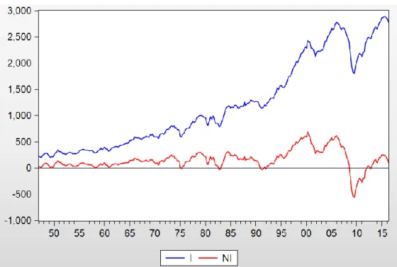
While the idea behind underconsumption makes sense, it is difficult to find evidence supporting such a mechanism, at least in the cycles of the last 50 years in the USA. In figure 1, it can be seen that the ratio between consumption and income actually seems to rise, instead of falling, before most depressions (marked in grey). Harvey (2014) and Goldstein (1999) provide further evidence confirming this problem.

(14)

9

Figure 1- Propensity to consume (ratio consumption/income) over US business cycles, 1947-2015 Source: FRED2

2.4.3. Hicks

An alternative explanation for crises also relying in the M-A model as its base is provided in the model by Hicks (1950). He assumes that investment has an autonomous component that grows at a constant rate overtime, besides the induced component determined by the accelerator. He additionally considers that output cannot exceed a certain full capacity level that also has a constant growth trend.

After an expansion has developed for some time along the lines of the M-A model, output eventually reaches its full capacity ceiling, which slows it down to the growth rate of full capacity output. The slowing down of output, because of the accelerator, implies a decrease in (induced) investment which, through the multiplier, causes a decrease in output, beginning a depression.

2

(15)

10

2.4.4. Overinvestment

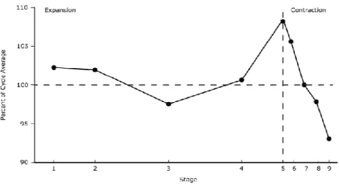
A third type of explanation for crises is that of the overinvestment model (Sherman, 1991, ch.11, based on Marx and Hayek). The factor that triggers the crisis is the increase in capital goods’ prices at a faster pace than consumer goods’ prices. This is a consequence of a rapidly increasing demand for capital goods in the boom, with which their supply cannot keep up. The result is a decrease in the profit rate, and thus investment and output. Note, however, that Sherman (2010) found evidence confirming this theory only for the prices of raw materials, and only in the cycles from 1970 to 2009. The prices for plant and equipment were observed to behave similarly to consumption goods’ prices.

In figure 2 it can be seen that, in the average business cycle in the USA from 1970 to 2001, the ratio between the prices of raw materials and general prices rises sharply before the contraction, which supports the idea behind overinvestment as a cause of crises, and the price of raw materials as the relevant variable in the model.

Figure 2- Ratio of raw materials prices to consumer good prices for the average business cycle in the

USA in the period 1970-2001. Stages 1 to 4 correspond to the expansion, stage 5 is the peak and stages 6 to 9 correspond to the depression

(16)

11

2.4.5. Reserve army

The reserve army model (Boddy & Crotty, 1975) provides a different explanation for crises. According to this model, as unemployment falls in expansions, workers’ bargaining power increases, which leads firms to accept their demands for higher wages (because they have now a much smaller “reserve army” to choose from). The consequence is an increase of wages above inflation, which increases the labor share at the expense of the profit share, thus leading to a decrease in the profit rate. This, in turn, brings investment down and causes output to start falling.

2.4.6. Profit Squeeze

Putting together the ideas of the three precedent models, Sherman (1991, ch.13) proposes a new model, known by the name of profit squeeze3. Its name refers to how the model explains crises: along the expansion, the profit is squeezed between revenues and costs. On the one hand, the revenue, which is output, decelerates because of the declining multiplier (from the underconsumption model). On the other hand, costs (the crucial types being the labor cost and the cost of raw materials) strongly increase in late expansion (see the separate explanations for the reserve army and the overinvestment models). This initially causes a deceleration and then a fall in profits and in the profit rate. As investment is determined by the latter, it also falls, which, because of the multiplier, causes a fall in output and the beginning of a depression.

It is worth noting the way how Sherman (1991) models the behavior of the profit share, which is a crucial variable in the model, not only because it is the vehicle introducing the

3

There is some confusion around this name: Goldstein (1999) defends a model that he calls “Cyclical profit squeeze” (of the reserve army type), claiming that Sherman’s model (which he calls nutcracker model) is not supported by data. Sherman (1991), however, uses both designations as synonyms. In this dissertation we will use the name “profit squeeze” to refer to Sherman’s model, as described in Sherman (1991).

(17)

12 reserve army theory in the model, but also because it determines the behavior of the multiplier. According to him, the profit share is a positive function of capacity utilization in the same period, on the one hand, and a positive function of unemployment lagged a given number of periods, on the other hand. The reason for unemployment to have this lagged effect on the profit share is that the bargaining of wages takes some time to produce effect in actual wages. This function permits to reproduce in the model the behavior of the profit share and, at the same time, provides an explanation for it. The result is a rapid increase of the profit share in early expansion (because wages are still low or even decreasing due to the time lag), and a deceleration in late expansion, as wages start increasing due to pressure from workers.

In the literature, there is some controversy around this model, especially in what regards the assumptions linked to overinvestment and underconsumption (see Goldstein, 1999). As was seen above, a simple observation of national accounts data suggests some problem with underconsumption. However, in what regards overinvestment, and the prices of raw materials in particular, there seems to be a contradiction between the results of Goldstein (1999) and what is shown in figure 2, from Sherman (2010).

While increases in production capacity are a function of the level of (net) investment, increases in output are a function of increases in investment. In late expansion, because investment has been growing since the recovery, net investment is at a very high level while the increases in investment cannot have this ascendant behavior4. This causes the paradox of investment (see above) to lose strength in late expansion, and eventually to be reversed. When this happens, utilization decreases. In the next period investment decreases too which, through the multiplier, begins a depression.

4

In the limit, investment will stop growing when utilization is forced to stabilize when it reaches its ceiling of 1

(18)

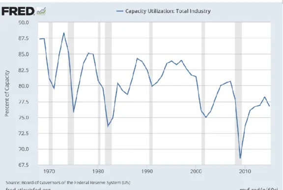
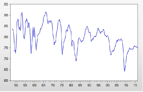
13 It is possible to find some support for this idea by a simple visual inspection of a plot of capacity utilization for the total industry in the USA in the last decades (figure 3). It can be observed that capacity utilization falls for some time before the majority of crises (marked in grey).

Figure 3- Capacity utilization in the total industry over US business cycles, 1967-2016 Source: FRED

2.5. The depression

The explanation for the depression provided by the M-A model is similar to its explanation for the expansion, but in reverse, with the difference that gross investment cannot fall below 0. If this lower bound is reached, investment stabilizes and so does output. This by itself can start a recovery.

(19)

14

According to the capacity utilization model, the initial drop in investment in the crisis causes output to fall. However, as long as net investment is still positive, the capital stock and productive capacity are rising. This causes a strong drop in capacity utilization, which further depresses investment and causes the output fall to continue. This happens until gross investment reaches its lower bound (its autonomous part). When this happens, output ceases to fall.

2.6. The recovery

The explanations for the recovery are essentially symmetric to those for the crisis. The difference is that, when investment is falling, the zero bound can limit its fall, while there is no upper limit when it is rising.

According to the M-A model, when gross investment reaches zero, it stops falling and thus the same happens with output. While the previous decreases in output determined negative net investments, the stagnation of output will determine null net investments (i.e. gross investment will assume a positive value, equal to depreciation). This means an increase in investment, which causes output to increase, through the multiplier, and the next expansion to begin.

2.6.2. Underconsumption

If we add to the M-A model the underconsumptionist assumption, there is an additional factor that helps to trigger the recovery. According to that assumption, the deepening of the depression causes the labor share to rise. The rise in the labor share leads to a higher propensity to consume and to a higher multiplier. This amplifies the effect of investment on output, making it easier for the economy to recover.

(20)

15

2.6.3. Hicks

This model relies on a growing autonomous investment to explain the recovery. After some time into the depression, investment eventually reaches its autonomous component, which causes it to start growing at the rate of autonomous investment. This small increase in investment is sufficient to determine an increase in output, via the accelerator, which marks the beginning of a new expansion.

2.6.4. Overinvestment

According to the overinvestment model, the same mechanism that triggers the crisis acts in reverse to trigger the recovery. As the depression deepens, the demand for raw materials falls sharply. Because their supply cannot decrease as fast, their prices tend to decrease. This decrease eventually stimulates the profit rate, which in turn stimulates investment and, through the multiplier, output.

2.6.5. Reserve army

In the reserve army model, the factor that increases the profit rate in the end of the expansion is the high unemployment. The reasoning is that high unemployment means a low bargaining power for the labor force, making it easier for companies to decrease wages. In turn, the lower wages depress the labor share and increase the profit share, thereby increasing the profit rate.

2.6.6. Profit squeeze

Along the depression, the labor costs and raw material costs decrease5, in the same way as they have increased along the expansion. On the other hand, the multiplier increases as the profit share decreases. Additionally, because gross investment cannot fall to negative values, it eventually stabilizes, stopping output to decrease further. All these factors contribute

5

(21)

16 to the increase in profits and the profit rate, which causes investment to increase and, through the multiplier, output to increase as well. This marks the end of the recession and the beginning of a new expansion.

According to the capacity utilization model, investment’s lower bound (autonomous investment) is crucial to explain recovery. In fact, when induced (as opposed to autonomous) investment reaches zero, it cannot fall much further. Therefore, investment eventually starts rising at the growth rate of its autonomous part, which causes output to increase too. While the production capacity can also rise via the increase in the capital stock (if autonomous investment exceeds depreciation), it will rise very slowly, because net investment is usually close to zero at this point. As a result, capacity utilization starts recovering and investment starts growing above the growth rate of its autonomous part once again, leading to the next expansion.

After the main views on endogenous business cycles have been exposed, we will now, based mainly on the capacity utilization model by Leão (2016) and the profit squeeze model by Sherman (1991), build a new model, joining together two different kinds of investment functions, corresponding to capacity utilization and the profit rate as its main determinants. The profit squeeze will bring to the capacity utilization model new mechanisms that are mainly relevant to explain the turning points of the cycle (crises and recoveries).

The model thus obtained will be tested by simulating business cycles and comparing the results with stylized facts.

(22)

17

3. Methodology

3.1. The model

The model derives from the capacity utilization model (Leão, 2016), and includes the assumptions of underconsumption, overinvestment and reserve army, based in the profit squeeze model by Sherman (1991). It has two fundamental equations corresponding to its two main mechanisms: on the one hand, the multiplier; on the other hand the investment function. It is built in discrete time, with a quarter as the time period.

Considering an open economy with government, then:

̅̅̅̅ ̅ (6)

where ̅̅̅̅ are net exports and ̅ is the government spending, both exogenous to the model and constant over time.

Now, if ̅ , where is the overall tax rate, then:

̅ ̅̅̅̅ ̅

̅ ̅̅̅̅ ̅ ̅ ̅̅̅̅ ̅

̅ (7)

where is the multiplier and ̅ ̅ ̅̅̅̅ ̅ is the autonomous part of output

According to the underconsumption theory, the marginal propensity to consume should be a negative function of the profit share, which implies that the multiplier should also be a negative function of that share. Because this reduces the number of parameters without having a significant impact in the results of the model, we will directly consider the multiplier a

(23)

18 negative linear function of the profit share. In order to simplify the model6, we will apply a time lag to the profit share, which should not make a significant difference in the results:

( )

(8)

The capital stock in a given period7 is the sum of the capital stock in the previous period and net investment in the current period:

₍₉₎

where is the depreciation rate, assumed to be constant overtime

In turn, assuming a constant technology, total production capacity is given by:

₍₁₀₎

where , the productivity of capital, is assumed to be constant overtime.

Capacity utilization is defined as:

(11)

which is subject to the constraint that , i.e.

The investment function includes the capacity utilization actual/desired gap lagged one period (as in Leão, 2016) and the profit rate, also lagged one period8:

( )

(12)

6

Having , which would happen if there were no time lag for in equation 8, would complicate the recurrence relation representing the model (see below) and render the simulations too cumbersome.

7_{Defined as the capital stock at the end of the period} 8

This implies that investment reacts to the changes in the profit rate after 3 months (1 quarter), which is consistent with the findings of Klein and Moore (1985), who found that profit rate expectations (which affect investment instantaneously) respond to the actual profit rate with a lag of three to four months.

(24)

19 subject to the constraint that . is the autonomous part of investment, related to factors other than capacity utilization or the profit rate.

The profit rate depends, on the one hand, on the profit share and capacity utilization (which follows from the identity in equation 59) and, on the other hand, on the relative price of raw materials (according to the overinvestment model):

( ) ( ) (

) (13) where is a price index for raw materials and is the implicit price deflator of the GDP.

The effect of the productivity of capital, assumed to be constant over the cycle, is included in the intercept, .

In turn, the profit share is determined by capacity utilization without a time lag and by unemployment with a certain time lag. The latter will be assumed to be one quarter:

(14)

Differently from Sherman (1991), who assumed unemployment as a function of output, we will assume it to be dependent on capacity utilization. This makes more sense because both unemployment and capacity utilization are bounded between 0 and 1, which does not happen with output. Therefore, we define unemployment as:

(15)

The relative price of raw materials is defined similarly to unemployment:

(

) (16)

9

Although the real function is in the form of a product, we will follow the approach of Sherman (1991), with a simple linear function also including the raw materials’ price ratio.

(25)

20 From the equations above, we can deduce, by substitution, a single equation for investment, in which it depends solely on capacity utilization lagged one and two periods:

( ) (17)

Or simply:

(18)

where , and

Considering the signs of the parameters ( and are negative), we can readily conclude that must be negative. As for , it is possible that it is positive or negative (the latter if the effect of is large enough), but, for the model to make sense, must still be positive. This yields an investment function in which capacity utilization has a positive effect with a one-period-lag and a negative effect with a two-period-lag.

For the simulation, we will use this simplified investment function. In fact, it makes no sense to include all the separate effects if there is no reasonable idea about their values in reality.

It is worth noting that, if , which happens, for example, if (i.e., if there is no effect of the profit rate on investment), then we have the investment function as in Leão (2016):

(19)

The model described above is not subject to growth in the long run, unlike what is observed in real economies. In a second step, we will introduce growth in the model by making autonomous investment and autonomous output grow at a constant rate ( ) overtime:

(26)

21

̅ ̅ (21)

Assuming this, it also makes sense that the sensibility of investment to capacity utilization and to the profit rate increase overtime at the same rate:

(22)

(23)

which implies that , and also grow at this rate:

(24)

where . The same reasoning applies for and

The investment function now becomes:

(25)

The multiplier function can be, as the investment function, expressed only in terms of the utilization rate:

( )

(26)

where , and . Because , then and .

(27)

22 (27)

Considering now the multiplier dependent on the profit share, the recurrence system becomes:

(28)

Finally, it is necessary to enforce that the conditions and are verified:

(29)

3.2. The simulation

The recurrence has no analytical solution (mainly because of the nonlinearity in of the capacity utilization equation). Therefore, only simulations are possible. These will be performed usingWolfram Mathematica, with the recurrence equation system above (equation 29). The simulated path of the variables other than and can be easily obtained from the latter.

As this dissertation has not the objective of calibrating the model for a real situation, the values chosen for the simulations are merely educated guesses. In fact, while we will use plausible parameter values whenever possible, the stress is put on how the model functions and what are the effects of changes in the parameters, rather than on creating a model capable of simulating a concrete real situation.

(28)

23 There are a total of 12 parameters in the model, besides the growth rate, and so it is impossible to thoroughly analyze the effects of all their possible combinations. The approach used will be the following:

1. There are four parameters ( , , and 10), whose plausible values can be known, using other works on the subject or performing simple estimations with data. These values will be the starting point to build the model in its simplest version (which is the one used in Leão, 2016, with ).

2. The values of the remaining 3 parameters ( , ̅ and ) will be defined in order to obtain a model generating constant business cycles, as similar to those observed in reality as the model permits. This, in practice, means that capacity utilization should not reach 1 and investment should not reach 0.

3. From this benchmark model, one parameter at a time will be changed and the resulting simulation will be observed in order to have an idea of how each parameter changes the result of the model.

4. For the parameters set to 0 in the benchmark model, it will be necessary to define a slightly different benchmark model where those parameters are different from 0. From this model they can be increased or decreased and the effect evaluated, just as the other parameters.

The estimation of was performed by simply dividing the real consumption of fixed capital by the real capital stock11 for the USA. The data were obtained from FRED. The time series thus obtained was simply averaged to give a rough estimate of 4% per quarter for .

10

represents the multiplier, if and are zero.

11

In the case of capital stock, as the original data are annual, a linear interpolation method was used to estimate data for each quarter.

(29)

24 The initial value for the desired utilization rate was based on the observation of the time series for the capacity utilization in the manufacturing industry for the USA, obtained from the US Federal Reserve website. The simple average of this time series is close to 0,8. The desired rate should be somewhat higher but, as the time series has lower values in the recent years, the value of 0,8 will be used.

As for , a time series was obtained from GDP, capacity utilization and capital stock using the following relation:

(30) The average for the USA for the last 60 years is close to 0,4, which will be the initial value used for .

Finally, in Lavoie (2014, p.369 and 380) it is implied a multiplier of 1,72. Based on the reasoning in Leão (2016), considering that 90% of the effect happens in one quarter, a value of 1,5 will be used for .

In the model with growth, a growth rate of 0,8% per quarter will be used, which is the quarterly average of GDP growth from 1947 to 2016 in the USA12.

All the sources of the data used can be consulted in table A1, in the appendix.

To solve the recurrence relation in equation 29, the first two pairs must be known. We will use as the two initial conditions.

The simulations performed in Mathematica will permit to obtain the time path of the key variables ( , , , , , , and ) of the model. Besides this, a plot of , points

12

(30)

25 will also be generated for up to 5000. This plot will be used to evaluate the performance of the model in the long run, as a substitute for the limit of the recurrence solution when , if this solution were indeed analytically available.

Additionally to the plots, an estimate of the period, amplitude and level of the cycles in the long run for , and will be computed. It will be assumed that, for , the long- run position was already reached. The level will be computed as the mean of the variables from to and the amplitude as the difference between maximum and minimum of the variables over the same time range. The period of the cycles will be estimated as the average difference in time between the first 5 peaks after .

The code used to obtain the simulations is presented in the appendix and can be copied from there directly into Mathematica to generate simulations of the model.

3.3. The effect of the additional assumptions in the base model

Because there are no estimates of the parameters of the model, it is not possible to fully understand how considering the additional assumptions of underconsumption, overinvestment and the reserve army changes the results. In order to fully observe these changes, it would be necessary that the model retained the separate parameters, but, as we argued, this would only make sense if there were some clues about their real values.

Nevertheless, it is possible to deduce the consequences of each of the theories in the values of , , and , as compared to the base model (where ):

 Underconsumption: The simplest underconsumption model requires at least

that . If we consider the effect of lagged unemployment on the profit share, then, additionally, .

(31)

26

 Reserve army: If the reserve army theory applies, then and .

 Overinvestment: In this case, . It should be noted that, while can be positive or negative, it is restricted by the condition . Otherwise the model would not make sense, because investment would be negatively affected by the capacity utilization rate lagged one period.

4. Results and discussion

4.1. General observations

The first thing that became apparent in the simulations was that the initial conditions for and , despite being necessary to run the simulation, do not affect the path of the variables after some time has passed. In fact, the model without a growth rate generates a stationary state, with the particularity that, for the right combinations of parameters, cycles with constant amplitude and period are present, for and and all the remaining variables.

The cycles are not synchronous for and , which was to be expected given the mechanisms behind the model. In fact, after the peak in , grows for some time before reaching its own peak. This is because, when utilization starts falling, net investment is still at its peak, and so the capital stock is increasing at the maximum rate.

It was observed that the model can generate three types of cycles:

1. Damped cycles: the economy oscillates with a smaller and smaller amplitude around a steady state

2. Constant cycles (or at least with cyclical patterns) without, for a significant length of time, (a) utilization reaching its upper bound (1) or (b) investment reaching its lower bound (0).

(32)

27 3. Constant cycles with periods during which either (a) or (b) are verified.

It should be said that the model does not generate cycles for every parameter combination, but also exponential growth paths (even with ) or chaotic results, especially for very extreme parameter values. We discarded this kind of simulations as originating in degenerate versions of the model and our attention was focused on the three situations described above, which correspond to a fairly large range of parameter values.

An economy in the first situation requires some kind of shock for the cycles to continue in the future, as happens for exogenous business cycle theories. The second situation is the most approximate to the real world: in fact, through all the History of national accounting, business cycles are always present and their amplitude does not seem to diminish overtime. The third situation is also compatible with the stylized fact that there is no decreasing tendency in business cycles’ amplitude. However, as can be seen by observing the time series for capacity utilization and investment since 1948 for the USA13, the economy never reaches a utilization level of 1 or an investment of 0. Because of this, situation 2 will be considered, throughout the simulations, the “desirable” result, in the sense that it generates the most realistic business cycles.

To define the benchmark model, which will be the reference from which all the other simulations will be compared, the three parameters for which plausible values could not be obtained were changed until a simulation consistent with the second situation above was achieved. The result of the simulation and the values for all the 7 non-null parameters in the benchmark model are displayed in figure 4.

13

(33)

28

Figure 4- Simulation results for the benchmark model

It is possible to see that the model is capable, in the long run (after the cyclic equilibrium is attained, roughly after 30 quarters in this case), of generating business cycles corresponding to the situation 2 described above. The cycles repeat unchanged overtime, as can be verified in the graph, for which 5 000 quarters (instead of the mere 200 shown in the other graphs) were computed. Capacity utilization never reaches 1 after the equilibrium is attained. As for investment, it just touches 0, and thus is not affected by the investment lower bound. However, given that the investment time series never touches 0 from 1948 to 2016, this result of the model does not fully match the data. Moreover, net investment for the same period does not fall below 0 for most of the business cycles (the only significant exception being the crisis of 2008)14, while in the simulation it is below 0 for some time in each cycle. In these conditions we did not manage to obtain a more satisfactory result. In fact, if net investment were always positive, there could not be constant cycles in capital. However, in the

14

See figures A1 and A2 in the appendix.

u a E 0 Y0 I0 F H A0 B0 D0 g n k1 u1 k2 u2 u a E 0 Y0 I0 F H A0 B0 D0 g 0.04 0.8 0.4 1.5 57 30 10 0 0 0 0 0 0 K u Y Max 277.97 0.87 80.06 Mean 241.29 0.62 59.47 Min 206.23 0.44 45.00 Amplitude 71.73 0.43 35.06

(34)

29 real world there is a growth trend that can partly explain this behavior of investment and net investment. While in this phase we did not include growth in the model, some sections below we will discuss this problem in the context of the complete model, including the growth rate.

4.2. Effects of the individual parameters

The benchmark simulation corresponds to a rather fragile situation in which the parameters are in a mutual equilibrium, such that the cycles do not dampen overtime neither are they so strong that the restrictions on investment and capacity utilization have a relevant role in keeping the variables within reasonable bounds, making the cycles unrealistic. In fact, once one of the parameters is changed the situation immediately changes, either to the damped cycles or to the opposite situation. In order to keep the model in this desirable parameter equilibrium, it is necessary to compensate the movement in one parameter by the movement of another one in the appropriate direction, so that the two effects balance.

The following table summarizes the main effects of changes in the parameters on the cycles resulting from the simulation. In order to lighten the table, was not included, given that its role is equal to that of (see equation 25).

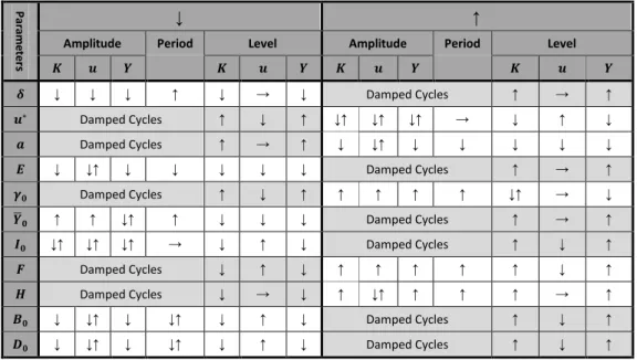
Table 1- Effect of a change in the parameters in the resulting cycles

P ar am ete rs ↓ ↑

Amplitude Period Level Amplitude Period Level

↓ ↓ ↓ ↑ ↓ → ↓ Damped Cycles ↑ → ↑ Damped Cycles ↑ ↓ ↑ ↓↑ ↓↑ ↓↑ → ↓ ↑ ↓ Damped Cycles ↑ → ↑ ↓ ↓↑ ↓ ↓ ↓ ↓ ↓ ↓ ↓↑ ↓ ↓ ↓ ↓ ↓ Damped Cycles ↑ → ↑ Damped Cycles ↑ ↓ ↑ ↑ ↑ ↑ ↑ ↓↑ → ↓ ̅ ↑ ↑ ↓↑ ↑ ↓ ↓ ↓ Damped Cycles ↑ → ↑ ↓↑ ↓↑ ↓↑ → ↓ ↑ ↓ Damped Cycles ↑ ↓ ↑ Damped Cycles ↓ ↑ ↓ ↑ ↑ ↑ ↑ ↑ ↓ ↑ Damped Cycles ↓ → ↓ ↑ ↓↑ ↑ ↑ ↑ → ↑ ↓ ↓↑ ↓ ↓↑ ↓ ↑ ↓ Damped Cycles ↑ ↓ ↑ ↓ ↓↑ ↓ ↓↑ ↓ ↑ ↓ Damped Cycles ↑ ↓ ↑

(35)

30 Any parameter, if changed in a certain direction, will determine the dampening of the cycles. If it is changed in the opposite direction, the cycles remain constant but the restrictions on and become more and more binding, resulting in long periods during which capacity utilization is 1 and/or periods during which investment is 0. As it was explained, both situations, while theoretically possible, are different from what happens in the real economy.

This behavior, common to all the parameters, could suggest that a variation of one of them can be entirely “neutralized” by an appropriate change of any of the others. As the table shows, this is not true: the effect in the shape of the cycles varies across the parameters in such a way that there are no two parameters whose effects either perfectly match or are the exact opposites15. As such, if two given parameters are changed so that the cycles remain equilibrated, it is likely that the shape of the cycles will change, because there are effects of the change in one parameter that cannot be evened out by a change in the other. Therefore, the benchmark model is only one example of the results that the model can yield while having constant cycles overtime not unrealistically “deformed” by the restrictions on and . This is important, because it means that the model has the necessary plasticity to reproduce the wide range of business cycle patterns that we see in the real world.

Some simulations were performed for each of the three additional theories (underconsumption, reserve army and overinvestment) considered in the model, whose effects in the parameters were already mentioned. As was argued, a full analysis of these theories and their impact on the results of the model is not possible in this dissertation, due to too many parameters whose real values are completely unknown. However, it is possible to investigate whether they can bring something new to the model.

15

Even in the case of and , while the directions of the effect fully match, their relative size may be different.

(36)

31 The results of the simulations performed can be consulted in the appendix (figures A4 to A7). It was found that only the underconsumption theory could significantly change the results of the model. In fact, if is negative, a new possible result appears: the model generates variable cycles, whose amplitude changes periodically overtime16_{. This new effect} comes from a new mechanism in the model introduced by the underconsumption theory: the multiplier depending on utilization, instead of being fixed. This creates a recurrence relation in the multiplier part of the model, which, mixed with the recurrence in the investment part, gives these rather complex results. This new characteristic of the model, if well explored, could be helpful in explaining business cycles with seemingly periodic amplitude, although, as we argued, its usefulness is limited by the lack of statistical evidence confirming the existence of the underconsumption mechanism in real economies.

In the case of the two other assumptions, the results obtained did not significantly differ from those obtained with only the base model. This does not mean that overinvestment and reserve army theories are useless. In fact, in a real situation, it would be interesting to know the relative strength of these forces in defining the business cycles, by estimating all the separate parameters of the model. In our case, as the effect of the operation of those two theories can be largely reproduced by simply changing the parameters of the base model, it is not possible to conclude about the importance of the theories without having some certainty about the values of the parameters.

4.3. The effect of growth

When a growth rate is included in the model, the constant cycles are superposed with an exponential path, for the variables in which this makes sense (for example, in the case of the cycles remain constant). This behavior approaches much more closely the real world, in

16

(37)

32 which business cycles start at higher and higher levels because of the long-run growth of the economy.

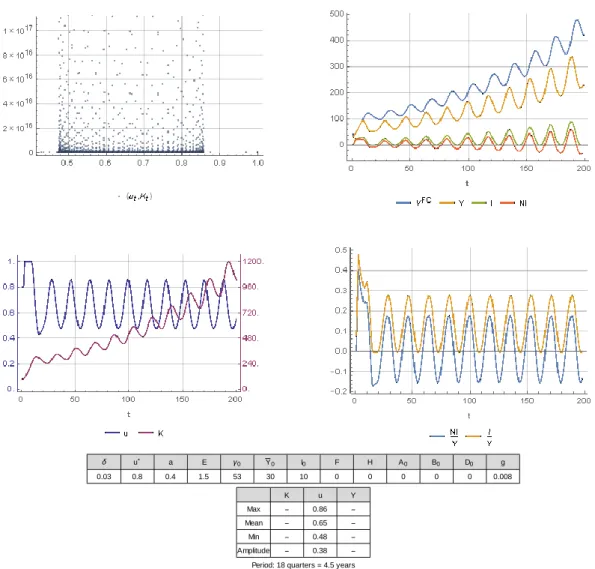
In the result of the simulation of the benchmark model with a growth rate of 0,8% per quarter (as computed from data for the USA), capacity utilization touched 1. This is understandable, as a long-run growth rate acts as a stimulus to utilization. The parameters were therefore slightly adjusted to make the simulation more realistic. It was found that the three flexible parameters ( , ̅ and ) were not enough to accomplish this: the rate of depreciation had to be reduced from 4% to 3% so that the cycles became acceptable according to the criteria already discussed. The result and the parameters used can be seen in figure 5.

Figure 5- Simulation results for the model including growth

0.03 u a E 0 53 Y0 I0 F H A0 B0 D0 g 0.008 n k1 u1 k2 u2 u a E 0 Y0 I0 F H A0 B0 D0 g 0.03 0.8 0.4 1.5 53 30 10 0.0001 0.00001 0 0 0.00001 0.008 K u Y Max 5.11 1019 0.86 1.45 1019 Mean 1.44 1018 0.65 3.68 1017 Min 592517. 00 0.48 135390. 00 Amplitude 5.11 1019 0.38 1.45 1019 Period: 18 quarters 4.5 years

0.03 u a E 0 53 Y0 I0 F H A0 B0 D0 g 0.008 n k1 u1 k2 u2 u a E 0 Y0 I0 F H A0 B0 D0 g 0.03 0.8 0.4 1.5 53 30 10 0 0 0 0 0 0.008 K u Y Max 0.86 Mean 0.65 Min 0.48 Amplitude 0.38

(38)

33 It can be seen that net investment is less negative as a percentage of when compared with the model without growth. Nevertheless, it still drops below 0 in every cycle. Additionally, the problem cannot be solved by increasing autonomous investment, as one could think. This is counterintuitive, but it can be understood considering that, while if autonomous investment is raised alone investment must follow, when this is done the constant cycles are replaced by damped cycles. Therefore, another parameter must be changed in order to balance the effect. The problem with the model is that, for all other parameters, this change ends up neutralizing the effect of the initial change in autonomous investment and, in the end, net investment continues to assume negative values. The long-run growth rate, at realistic levels, helps to raise investment, but only at very high levels (in excess of 5% per quarter or 20% per year) is it able to fully solve the problem.

(39)

34

5. Conclusions

In this work, a business cycle model was built with the aim of joining the main views in the literature about endogenous cycle theories. This was done by taking to a further step what Sherman (1991) did in his profit squeeze model and including capacity utilization as a crucial part of the investment function. This synthetic model permits to systematize in a mathematic form the existing views on endogenous business cycles and intends to serve as a base on which new theories can be developed.

It was found that the model by Leão (2016) is capable of generating constant business cycles overtime, for the right sets of parameters. Therefore, this model, while relying in very simple assumptions and a single cycle-explaining mechanism, is still capable of generating full constant cycles in the long run. Despite that we had not obtained estimates for all the parameters of the model, still most of the values used were fairly plausible guesses, and at the very least we can say that investor responses to fluctuations in the deviation of capacity utilization from its desired level can play a very important role in the mechanism that generates business cycles in the real world. Moreover it was shown that the model has a significant flexibility, permitting to obtain cycles with varying characteristics, which is another sign of a good explanatory power.

As for the additional assumptions (underconsumption, overinvestment and reserve army) they did not significantly change the kind of results that can be obtained with the model (with the exception of underconsumption). However, as we argued, this does not mean that the theories are useless, but merely that the extent to which they determine business cycles in real economies can only be known after the parameters of the model are appropriately estimated.

(40)

35 Regarding underconsumption, the variable multiplier, under the appropriate parameter values, permitted to generate cycles whose amplitude varied periodically overtime, instead of being constant. While this is interesting, it is also true that solid statistical evidence supporting the existence of the underconsumption mechanism in reality is yet to be found, which naturally undermines the practical utility of this finding.

Additionally, it was shown that the model can easily incorporate a long-term growth trend, which further increases the potential realism of the results.

The main problem that was found regarding the realism of the simulations was that of the lower bound of investment. In fact, while in the last 50 years in the USA gross investment has never reached 0 and net investment has seldom been negative, we did not manage to reproduce such a behavior in the simulations.

It must also be stressed that, while we tried to use parameter values as plausible as possible, in some cases they were totally unknown, and so it remains to be studied how well the model can simulate a concrete economic situation. For that, the estimation of the model parameters would be needed, which would be the additional step necessary for our work to be complete.

Finally, it should be noted that our work largely ignored the theories centered on the importance of the financial conditions in explaining business cycles. These have a potentially important role in the development of economic cycles in the real world and their inclusion in the model may significantly reduce the problems that we found and improve the realism which the model is capable of.

(41)

36

References

Boddy, R., & Crotty, J. (1975). Class Conflict and Macro-Policy. Review of Radical Political

Economics, 7(Spring), 1-17.

Goldstein, J. (1999). The Simple Analytics and Empirics of the Cyclical Profit Squeeze and Cyclical Underconsumption Theories: Clearing the Air. Review of Radical Political

Economics, 31(2), 74-88.

Harvey, J. (2014). Using the General Theory to Explain the U.S. Business Cycle, 1950-2009.

Journal of Post Keynesian Economics, 36(3), 391-414.

Hicks, J. (1950). A Contribution to the Theory of the Trade Cycle. New York: Oxford University Press.

Keynes, J. M. (1936). The General Theory of Employment, Interest and Money. London: Macmillan.

Klein, P., & Moore, G. (1985). Monitoring Growth Cycles in Market-Oriented Countries:

Developing and Using International Economic Indicators. Cambridge Massachusetts:

Ballinger.

Lavoie, M. (2014). Post-Keynesian Economics: New Foundations. Cheltenham: Edward Elgar. Leão, P. (2016). A Post-Keynesian model of the business cycle. Paper presented in Berlin at the

conference "Towards Pluralism in Macroeconomics? 20 Years-Anniversary Conference of The FMM Research Network".

Minsky, H. (1982). Can "It" Happen Again? Essays on Instability and Finance. New York: M. E. Sharpe.

Samuelson, P. (1939). Interactions between the multiplier analysis and the principle of acceleration. Review of Economic Statistics, 21(May), 75-78.

Sherman, H. (1991). The Business Cycle: Growth and Crisis under Capitalism. New Jersey: Princeton University Press.

Sherman, H. (2010). The Roller Coaster Economy: Financial Crisis, Great Recession and the

(42)

37

Appendix

Figure A1- Quarterly gross and net investment in the US from 1947 to 2016 (billions of 2009 dollars) Source: FRED

Figure A2- Quarterly gross and net investment as a proportion of GDP in the US from 1947 to 2016 Source: FRED

(43)

38

Figure A3- Quarterly capacity utilization rate for the manufacturing industry in the US from 1948 to 2016

Source: FRED

Table A1- Sources of the data

Variable Period Source Description

1947q1

2016q2

FRED

https://fred.stlouisfed.org/series/GDPC1

Billions of Chained 2009 Dollars, Quarterly, Seasonally Adjusted Annual Rate

1947q1

2016q2

FRED

https://fred.stlouisfed.org/series/GPDIC96

Real Gross Private Domestic Investment, 3 decimal, Billions of Chained 2009 Dollars, Quarterly, Seasonally Adjusted Annual Rate

1950

2014

FRED

https://fred.stlouisfed.org/series/RKNANP USA666NRUG

Capital Stock at Constant National Prices for United States, Millions of 2011 U.S. Dollars, Annual, Not Seasonally Adjusted 17

1947q1

2016q2

FRED

https://fred.stlouisfed.org/series/A262RX1 Q020SBEA

Real consumption of fixed capital, Billions of Chained 2009 Dollars, Quarterly, Seasonally Adjusted Annual Rate

1948q1

2016q2

Federal reserve

http://www.federalreserve.gov18

Industrial Production and Capacity Utilization for Aug 16, 2016

1947q1 2016q2

FRED

https://fred.stlouisfed.org/series/GDPDEF

Gross Domestic Product: Implicit Price Deflator, Index 2009=100, Quarterly, Seasonally Adjusted

17

The capital stock had to be adjusted from annual to quarterly frequency (linear interpolation), from 2011 to 2009 dollars (using IPD) and converted from millions of dollars to billions of dollars

18

(44)

39

Code used in Mathematica to run the simulations

TwoAxisPlot[a_, range_, imgs_] :=

Module[{fgraph, ggraph, frange, grange, fticks, gticks}, {fgraph, ggraph} =

MapIndexed[

ListPlot[#, Axes -> True, Joined -> True, GridLines -> Automatic, ImageSize -> imgs, AxesLabel -> {"t", "t"},

PlotRange -> range[[#2[[1]]]],

PlotStyle -> ColorData[1][#2[[1]]]] &, a]; {frange, grange} = (PlotRange /. AbsoluteOptions[#, PlotRange])[[ 2]] & /@ {fgraph, ggraph}; fticks = N@FindDivisions[frange, 5]; gticks =

Quiet@Transpose@{fticks,

ToString[NumberForm[#, 2], StandardForm] & /@ Rescale[fticks, frange, grange]};

Show[fgraph, ggraph /.

Graphics[graph_, s___] :> Graphics[

GeometricTransformation[graph,

RescalingTransform[{{0, 1}, grange}, {{0, 1}, frange}]], s], Axes -> True, FrameLabel -> {"t"},

Frame -> {True, True, False, True},

FrameStyle -> {ColorData[1] /@ {1, 2}, {Automatic, Automatic}}, FrameTicks -> {{fticks, gticks}, {Automatic, Automatic}}]];

Manipulate[

Grid[{{GraphicsGrid[{{ListPlot[ b = RecurrenceTable[{{u[1 + t],

k[1 + t]} == {Min[(e + f u[t] + h u[t - m + 1])/( a k[t]) (Max[\[Delta] k[t] + (1 + g)^(

t + 1) (i0 - \[Gamma]0 w +

a0 + (\[Gamma]0 + b0) u[t] + d0 u[t - m + 1]), 0] + y0 (1 + g)^(t + 1)), 1],

k[t] (1 - \[Delta]) +

Max[\[Delta] k[t] + (1 + g)^( t + 1) (i0 - \[Gamma]0 w +

a0 + (\[Gamma]0 + b0) u[t] + d0 u[t - m + 1]), 0]}, {k[1], u[1]} == {k1, u1}, {k[2], u[2]} == {k2, u2}, {k[3], u[3]} == {k1, u1}, {k[4], u[4]} == {k2, u2}, {k[5], u[5]} == {k1, u1}, {k[6], u[6]} == {k2, u2}, {k[7], u[7]} == {k1, u1}, {k[8], u[8]} == {k2, u2}, {k[9], u[9]} == {k1, u1}, {k[10], u[10]} == {k2, u2}}[[1 ;; m + 1]], {u, k}, {t, 1, 5000}],

ImageSize -> 330, PlotMarkers -> {Automatic, 3}, GridLines -> Automatic,

PlotLegends ->

Placed[{"(\!\(\*SubscriptBox[\(u\), \