1 Notes on the OLG Model

1

Notes on the OLG Model

1.1

Introduction

The overlapping generations (OLG) model, introduced by Sameulson (1958), is a dynamic economic model with many interesting properties. It contains agents who are born at di®erent dates and have ¯nite lifetimes, even though the economy goes on forever. This induces a natural heterogeneity across individuals at a point in time, as well as nontrivial life-cycle considerations for a given individual across time. These features of the model can also generate di®erences from models where there is a ¯nite set of time periods and agents, or from models where there is an in¯nite number of time periods but agents live forever. In particular, competitive equilibria in the OLG model may not to be Pareto optimal. A closely related feature of the model is that it has a role for ¯at money. This means we can use OLG models to address a variety of substantive issues in monetary economics.

1.2

The Basic Model

Suppose that t = 1;2; : : :, and that at every date t there is born a new generationGt of individuals who live for two periods. More realistic (longer) lifetimes can be studied, but two periods is the simplest case where the generations overlap. There is also a generation G0 around at t = 1 who

only live for one period, called the \initial old." For now, every generation consists of a [0;1] continuum of homogeneous agents. Let ct1 and ct2 denote

consumption of an individual from Gt, t ¸ 1, in the 1st and 2nd periods of life, and lete1 and e2 denote his (time-invariant) endowments in the 1st and

2nd periods of life. His utility function u(ct1; ct2) is strictly increasing and

with only e2.

One can de¯ne aWalrasian Competitive Equilibrium(WCE) for this econ-omy as follows. Letptbe the price of a unit of the consumption good at date

t. Now clearly every member of generation G0 simply consumes his

endow-ment, c02 = e2. For all t ¸ 1, every member of Gt maximizes u(ct1; ct2)

subject to

ptct1+pt+1ct2 =pte1+pt+1e2 (1)

andctj ¸0.1

We always write budget constraints with strict equality because

u is strictly increasing. Then a WCE is a sequence of prices and allocations fpt; ct1; ct2gsuch that: c02 =e2; given fptg, (ct1; ct2) solves the maximization

problem of Gt for all t¸1; and markets clear in the sense that for all t

ct1+ct_¡1;2 =e1+e2: (2)

One can also de¯ne aRecursive Competitive Equilibrium(RCE) as follows. Let st denote savings or loans by a member of Gt at t, and Rt the gross (principal plus interest) return on savings between t and t+ 1. Then for all

t¸1, every member of Gt maximizesu(ct1; ct2) subject to

ct1 = e1 ¡st (3)

ct2 = e2 +Rtst (4)

and ctj ¸ 0.2

A RCE is a sequence fRt; ct1; ct2g such that: c02 = e2; given

1_{We could write (1) more generally as}P

jpjctj=

P

jpjetj, where ctj is the

consump-tion andetjis the endowment in periodjof an agent born att, but it is obvious from the

speci¯cation of preferences and endowments thatctjandetjare nonzero only atj=tand

j=t+ 1. This means that we do not have to worry if the (otherwise in¯nite) summations converge when we write the individual budget constraint. However, if we try to price a point in the commodity space withctj>0 for in¯nitely manyj, convergence becomes an

issue (see below).

2_{As in the previous footnote, we could write the budget constraints as}

fRtg, (ct1; ct2) solves the maximization problem of Gt for all t ¸ 1; and (2)

holds for all t.

An immediate result is that WCE and RCE are equivalent concepts: that is, the sets of WCE and RCE allocations are the same. To see this, note that the only di®erence in the two de¯nitions is in the budget constraints; but, by eliminatingstfrom (3) and (4) and setting Rt=pt=pt+1;these two recursive

constraints are equivalent to (1). This is a very general result: versions of this equivalence between WCE and RCE hold in much more complicated models, including those where di®erent agents have di®erent (possibly in¯nite) life times, and even including those where there is uncertainty.

The next result is that the only equilibrium allocation here is autarchy: (ct1; ct2) = (e1; e2) for allt. To verify this, ¯rst note that homogeneity implies

no trade within a generation.3

Then note that in any equilibrium c02 = e2,

and combined with market clearing this implies c11 = e1. Then the budget

constraints imply c12 = e2, and so on, so that (ct1; ct2) = (e1; e2) for all t.

From the ¯rst order condition from the individual maximization problem,

for every date j, but the speci¯cation of preferences and endowments means that only (3) and (4) are relevant. Generally, if agents live N periods there will be N relevant constraints. Also, if utility is additively separable, we can write the individual problem as a dynamic program with state variable st¡1, control st, and value functions de¯ned

recursively via Bellman's equation

Vt(st¡1) = max

st

fU(etj¡stj+Rj¡1stj¡1) +¯Vt+1(st)g;

and the terminal conditionVT+1(sT¡1) = 0, whereT is the date at which the individual

dies. This should help to bring out the connection between RCE in the OLG model and in the neoclassical growth model.

3_{With homogeneity every member of G}

t chooses the same st, and since members of

Gt are the only ones in the credit market at t, equilibrium requires st = 0. In the next

the (constant) RCE interest rate is given byRt=¹(e1; e2) for all t, where¹

is the marginal rate of substitution function

¹(c1; c2) =

u1(c1; c2)

u2(c1; c2)

: (5)

Similarly, the WCE price sequence is given by pt=pt+1 =¹(e1; e2), where we

normalize p1 = 1 by appropriate choice of numeraire.

An interesting property of the OLG model is that equilibria may not be Pareto optimal. For example, suppose (e1; e2) = (1;0) and u(ct1; ct2) =

ct1+ct2, for allt ¸1 (this example may seem special because the indi®erence

curves are linear, but it will be clear below that the point is general). Then the autarchy allocation is Pareto dominated by (ct1; ct2) = (0;1) for all t,

since members of G0 are strictly better o® and members of Gt are no worse

o®. How is this possible, given that the ¯rst welfare theorem says competitive equilibria are always e±cient? Evidently the ¯rst welfare theorem does not apply in the OLG model, and it worth seeing why.

Generally, the standard proof (for ¯nite economies) that competitive equi-libria are e±cient proceeds as follows. Suppose by way of contradiction that an equilibrium allocation is dominated by some alternative allocation (chg), where hindexes households andg indexes goods. Then Pgpg(chg¡ehg)¸0

for everyh, with strict inequality for someh(because a bundle that is as least as good must cost at least as much and a bundle that is strictly better must cost strictly more). Adding over households, we havePh

P

gpg(chg¡ehg)>0.

Interchanging the summations, we have Pgpg P

h(chg ¡ehg) >0, which

im-plies Ph(chg ¡ehg)>0 for some good g. This last inequality violates

feasi-bility. In the OLG model, however, because the sets of goods and agents are in¯nite we cannotin general interchange the summations, and the argument breaks down.4

4_{In fact, when the model is not ¯nite, expressions like} P

In the above argument, the interpretation of Ph P

gpg(chg ¡ehg) > 0

is that people are spending more than their combined income, and the in-terpretation of Ph(chg ¡ehg) > 0 is that people are consuming more than

their combined endowment of good g. In the OLG model, if equilibrium is dominated by an alternative allocation then it is true that people would have to spend more than their income to buy it, but this does not mean that they would have to consume more than is feasible. Consider again the example with (e1; e2) = (1;0) and linear utility, for which pt = 1 for all t

in equilibrium. Given the alternative allocation (ct1; ct2) = (0;1), if we sum

the analogue of pg(chg¡ehg) ¯rst over goods and then over agents we get 1, but if we sum ¯rst over agents and then over goods we get 0; the alternative allocation does cost too much but it does not violate feasibility.

This is not to say that equilibrium in the OLG model is always ine±cient. We now show that, with strictly convex indi®erence curves, the unique equi-librium allocation is Pareto optimal if and only if the marginal rate of substi-tution at the endowment point is bigger than unity,¹(e1; e2)¸1. To simplify

the presentation, we assumee1 >0, and take for granted that we must treat

everyone within a generation the same. First, suppose ¹(e1; e2) < 1. To

show autarchy is ine±cient, consider the alternative allocation (ct1; ct2) =

(e1¡"; e2+") for all t¸1 and c02=e2+", where "2(0; e1]. Clearly this is

be well-de¯ned. This is why in in¯nite dimensional economies we often de¯ne budget constraints by means of a continuous linear functionalv that maps the commodity space into the real numbers (following Debreu 1958). Thus,v(c) is the value of any bundlec. The proof in the text goes through in in¯nite dimensional economies if we replace summations likeP_gpg(chg¡ehg) with expressions like v(ch¡eh). We can always represent v as an

inner product ¡that is, there always exists a p such thatv(c) =P_gpgcg for all c ¡if

Figure 1: Ine±cient Equilibrium

feasible and every member of G0 is better o®. As shown in Figure 1, as long

as ¹ <1 there is some " > 0 such that every member of Gt is better o® for

t¸1.

Now consider the case where ¹(e1; e2) ¸ 1, and suppose the autarchy

allocation is ine±cient. Then there is some alternative allocation (ct1; ct2)

thatu(ct1; ct2)¸u(e1; e2) for all agents, with strict inequality for some agent.

Let t be the ¯rst date at which the allocation di®ers from autarchy. We cannot have the old attconsume less thane2, since then they would be worse

o®, and so we must have e1¡ct1 ="t >0. Then we must have ct2¡e2 not

only positive, but bigger than "t, because ¹ ¸ 1, and so feasibility dictates

e1 ¡ct+1;1 = "t+1 > "t. Continuing in this fashion we get an increasing

sequence "t of transfers from the young to the old. This sequence cannot converge (why?); hence, there is some date T such that "T > e1, which is

infeasible.

1. In fact, nothing in the argument depends on (e1; e2) denoting the

endow-ment or the the equilibrium allocation. Hence, we can conclude that any time-invariant allocation (c1; c2) is Pareto optimal if and only if¹(c1; c2)¸1.

Moreover, the ¯rst part of the proof applies even if the allocation is not time-invariant: as long as ¹(ct1; ct2) ¸ 1 for all t, all individuals prefer

(ct1¡"; ct2+") for some " >0, and this is feasible as long as ct1 is bounded

away from 0.

The ine±ciency of equilibria when ¹ < 1 can be explained as follows. The rate at which society can trade c1 for c2 is unity, since we can freely

transfer from the young to the old. If we set the interest rate to Rt = 1, then¹ <1 implies individuals want to save ¡but saving is inconsistent with equilibrium. To see why, note that if G1 saves then c11 < e1, which implies

by virtue of (2) that c02 > e2, and this violates the budget constraint of the

initial old. Hence there is no scope for savings in equilibrium, even though savings is both feasible and desirable from the point of veiw of soctiety. In the next section we describe a way to allow the initial old to consume more than e2, and therefore the young to consume less that e1, so that they can

save, in equilibria with money.

It is worth remarking at this stage that the potential ine±ciency of com-petitive equilibrium in the model has nothing to do with the fact that agents overlap in a way that prevents them from getting together at datet = 1 and exploiting all possible gains from trade. That is, the result is not due to the fact that at date t the only feasible trades are between Gt¡1 and Gt. This

We close this section with an extension of the model that allows popula-tion to change. Letnt be the size of generationt, and assument=°nt_¡1 for

allt, for° >0. Now feasibility (market clearing) requiresntct1+nt_¡1ct_¡1;2 =

nte1+nt_¡1e2, or

°ct1+ct_¡1;2 =°e1+e2; (6)

for allt, which generalizes (2). Again the unique equilibrium is autarchy, but now the techniques used above imply that it is Pareto optimal if and only if

¹(e1; e2)¸°.

With population growth, society can transfer resources across time at rate

°, by taking one unit each from the young agents and distributing the pro-ceeds to the old agents. In equilibrium, zero savings requires Rt =¹(e1; e2).

If ¹(e1; e2) < ° then at rate ° agents would like to save, but in equilibrium

they cannot. The case ¹ ¸ ° is sometimes referred to as the \Classical case" (because classical results, like the optimality of competitive equilib-rium, hold), and the case ¹ < ° is referred to as the \Samuelson case" (presumably because he thought it up).

1.3

Money

Into the model described above, we now introduce a constant amount M of ¯at money, held in period 1 by the initial old G0. By de¯nition, ¯at money

is an object that has no intrinsic (consumption) value, but could potentially have exchange value. Letqtbe the value of money at datet. Ifq1 >0 then the

initial old can consume c02 =e2+q1M > e2 without violating their budget

constraint. Let every other agent in Gt, t ¸ 1, solve the same problem as before, maximizingusubject to (1) andct1; ct2 ¸0. Then a WCE with money

is sequence of prices and quantities fpt; qt; ct1; ct2gsuch that: c02=e2+q1M;

and the market clearing condition (2) holds for all t.5

It is more illuminating to discuss money in a recursive setting. In this case G0 still consumes c02 = e2 +q1M; but for all t ¸ 1, Gt maximizes

u(ct1; ct2) subject to

ct1 = e1¡qtmt¡st (7)

ct2 = e2+qt+1mt+Rtst; (8)

and mt; ct1; ct2 ¸0, where mt is interpreted as savings in terms of dollars or

the demand for money. If qt>0 we can combine (7) and (8) into

(ct2 ¡e2) +Rt(ct1¡e1) =qtmt

à qt+1

qt ¡Rt !

:

Now qt+1

qt > Rt implies mt = 1 and

qt+1

qt < Rt implies mt = 0, neither

of which are consistent with a monetary equilibrium (which will be seen to require mt = M for all t). Hence, a monetary equilibrium requires the \arbitrage condition" qt+1

qt =Rt.

Given qt+1

qt = Rt, individuals do not care whether they save in terms of

money or loans, only about total savings, qtmt+st. Moreover, assuming ho-mogeneous individuals in each generation, there are no loans in equilibrium:

st = 0. We will see below that if we relax the homogeneity assumption there can be within-generation lending as well as savings in terms of money, but for now we set st= 0 and write (7) and (8) as

ct1 = e1¡qtmt (9)

ct2 = e2+qt+1mt+Rtst: (10)

5_{In this de¯nition, the market clearing conditions are in terms of the consumption good}

Then a RCE with money is sequence fqt; ct1; ct2g such that: c02 =e2+q1M;

given fqtg, (ct1; ct2) solves the maximization problem of Gt for all t¸1; and

(2) holds for all t. Alternatively, as long as qt > 0, we can replace (2) by

mt =M, since we know (by Walras' law) that the goods market clears if and only if the money market clears.6

This is the framework within which we will usually discuss monetary issues in what follows. Given qt, the nominal price level is Pt = 1=qt for all t. If qt = 0 (Pt = 1) for all t we have a nonmonetary equilibrium, which is equivalent to the unique equilibrium in the model without money. It is a desirable property of a monetary theory that nonmonetary equilibria exist as special cases, since a prerequisite for ¯at currency to have value is that individuals believe that it will. We are interested now in monetary equilibrium, which requires qt >0 for somet. Notice that if qt>0 for some

t then qt > 0 for all t. This follows because qt = 0 implies the demand for money is 0 att¡1: who would give up resources for something that cannot be used in either consumption or trade? If the demand for money at t¡1 is 0 then qt¡1 = 0, and so on.

With qt > 0, we can insert (9) and (10) into the utility function and di®erentiate to get the ¯rst order condition for an interior solution,

¹(e1¡qtmt; e2+qt+1mt) =

qt+1

qt ; (11)

where¹(c1; c2) is the marginal rate of substitution function. The solutionmt

to (11) gives the money demand function as long as 0< mt < e1=qt; the ¯rst

inequality is true by de¯nition in a monetary equilibrium, and the second we can guarantee by assuming¹(c1; c2)! 1as c1 !0.

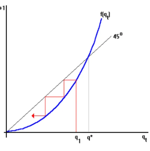
If we use the equilibrium condition mt = M, (11) implicitly de¯nes a di®erence equation, qt+1 = f(qt). A monetary equilibrium is completely

6_{Even thoughs}

characterized by a bounded sequencefqtgsatisfying this di®erence equation, a special case of which is asteady state, or a solution toq =f(q). We require

qt bounded since otherwise qtM eventually exceeds e1 + e2, which means

that at some date the agents holding the money will buy more than existing resources, and this violates feasibility. Notice that we do not have any intial condition for qt; we can set q1 arbitrarily, and the resulting path given by

qt+1=f(qt) will be an equilibrium as long as it remains bounded.

In general, the equation qt+1 = f(qt) satis¯es f(0) = 0 and f0(0) =

¹(e1; e2). We claim thatf0(0)¸1 implies that there is no solution tof(q) =q

while f0_{(0) =¹(e}

1; e2)<1 implies that there is exactly one solution. To see

this, note that solutions to f(q) =q satisfy T(q) = 0, where

T(q) =¡u1(e1¡qM; e2+qM) +u2(e1¡qM; e2+qM):

Since T0 _{< 0, there cannot be more than one solution to T(q) = 0. Since} T(q)<0 for q near e1

M, there exists a solution if and only if T(0)>0, which

holds if and only if ¹(e1; e2) < 1. Hence, a monetary steady state exists if

and only if¹(e1; e2)<1, which is exactly the condition for the nonmonetary

equilibrium being ine±cient.

We leave as an exercise veri¯cation of the following generalization of these results. Suppose there is population growth at rate °; then ¹ ¸ ° implies the nonmonetary equilibrium is Pareto optimal and no monetary steady state exists;¹ < ° implies the nonmonetary equilibrium is not Pareto optimal and a monetary steady state exists.

Consider an example with thelog-linearutility function,u(c1; c2) = log(c1)+

¯log(c2). This allows us to solve (11) explicitly for the money demand

func-tion,

mt=m(qt; qt+1) =

¯e1qt+1¡e2qt

qtqt+1(1 +¯)

; (12)

demand is zero. Notice that e2=¯e1 = ¹ is exactly the marginal rate of

substitution at the endowment point.

Consider ¯rst the special case where e2 = 0; then qt+1 drops out of (12)

and so mt=M implies

qt = ¯e1

(1 +¯)M ´q ¤

for all t. Hence, in this special case there exists a unique monetary equilib-rium and it is a steady state. The nominal price level,

Pt= 1 +¯

¯e1

M ´P¤_;

is proportional to M, as predicted by the \quantity theory." Real balances, denotedSt =qtM, are constant at St =S¤ _{=¯e1=(1 +¯).}

The case e2 = 0 is somewhat special, because with log-linear utility it

implies the demand for real balances is a constant fraction of e1 regardless

of next period's price level, and it is because of this that there always exists a unique monetary equilibrium. If e2 >0, then (11) can be rearranged as

qt+1 =f(qt) =

e2qt

¯e1¡(1 +¯)M qt

: (13)

An equilibrium is given by any bounded solution to (13). In this case, f0_{(q) >0, f}00_{(q)>0, and f(q)! 1 as q !¯e}

1=(1 +¯)M.

As always, if f0_{(0) = ¹ < 1 then there is a unique monetary steady state}

with

qt= ¯e1¡e2 (1 +¯)M ´q

¤_;

as shown in Figure 2; if f0_{(0) = ¹ ¸ 1 then there does not exist a steady}

state with q >0.

We now consider monetary equilibria that are not steady states. Suppose

¹ < 1, so that a monetary steady state q¤ _{exists, as shown in Figure 2 (if}

Figure 2: Dynamic Monetary Equilibria

any initial q1 > q¤, (13) implies qt ! 1; hence, sequences beginning with a

value of money in excess of q¤ _{cannot be equilibria. But for any initial q}

1 2

(0; q¤_{), (13) impliesqt!0 monotonically. Hence, there exist a continuum of}

bounded solutions to (13), indexed byq1 2(0; q¤), and therefore a continuum

of monetary equilibria. Counter to the quantity theory, these nonstationary equilibria are characterized by in°ation, even though the money supply is constant, since Pt ! 1 as qt ! 0. In°ation in this case is due to self-ful¯lling expectations that the value of money will fall. In the limit, the value of money goes to 0 and economy ends up in autarchy.

way: the fraction ®1 of the agents havee1 = 1 and e2 = 0, while the fraction

®2 = 1¡®1 havee1 = 0 ande2 = 1. Lets1tand s2tdenote the (real) savings

of the two types from generation Gt.

Consider nonmonetary equilibria. The ¯rst order condition

¹(e1¡st; e2+Rtst) =

e2+Rtst

e1¡st

=Rt

implies savings for the two types are given by s1t = 1=2 and s2t =¡1=2Rt.

The equilibrium condition that the loan market clears is 0 = ®1s1t+®2s2t,

which impliesRt=®2=®1 for allt. From our general welfare results we know

that®2 ¸®1 implies¹=R¸1 and the equilibrium is Pareto optimal, while

®2 < ®1 implies¹=R <1 and is not. In the latter case, there exists a Pareto

optimal monetary steady state with R = 1, s = 1=2, and qM = ®1 ¡1=2.

Hence, we see that with heterogeneity the model admits equilibrium where money and private loans coexist, although only if they bear the same rate of return.

1.4

Changes in the Money Supply

In this section we relax the assumption that the money supply is constant, by allowing it to change according toMt+1 =zMt. We assume for now that

the new is money distributed to members ofGt at datet+ 1 as a lump sum transfer,¿t(other ways of introducing new money are also considered below). An agent born at t ¸1 maximizes u(ct1; ct2) subject to

ct1 = e1¡qtmt (14)

ct2 = e2+qt+1(mt+¿t): (15)

Taking the ¯rst order condition for an interior solution, and then inserting the equilibrium conditionsmt=Mt and ¿t= (z¡1)Mt, we have

¹(e1¡qtMt; e2+qt+1Mt+1) =

qt+1

Equivalently, in terms of real balances St=qtMt, we have

¹(e1¡St; e2+St+1) =

St+1

zSt (16)

In the log-linear case, the generalization of (13) is

qt+1 =

e2qt

¯e1¡(z+¯)Mtqt

: (17)

Since Mt is changing with t, there does not exist constant q steady state; but we can look for the natural generalization in which the quantity theory implies Pt = ©Mt for some © >0 for all t. Inserting 1=qt = ©Mt into (17), we ¯nd

© = z+¯

¯e1¡ze2

:

Thus, © > 0 if and only if z¹ < 1, where ¹ = e2=¯e1. This generalizes the

condition for a monetary steady state derived above withM constant,¹ <1. To look for equilibria that do not satisfy the quantity theory, it is con-venient to work with real balances St rather than the value of money qt. Multiplying both sides of (17) by Mt+1 and simplifying, we have

St+1 =

ze2St

¯e1¡(z+¯)St

´f(qt); (18)

generalizing the functionf de¯ned above. In particular, there exists a steady state S¤ _=f(S¤_{), where}

St= ¯e1¡ze2

z+¯ ´S

¤_;

if and only if z¹ <1. Of course,S¤ _{corresponds the quantity theory}

equilib-rium derived above. Also, for any initial S1 2 (0; S¤), the sequence St is an

Mt.7

Returning to the quantity theory equilibrium, where St =S¤_{, we have}

c¤

1 =

z(e1+e2)

z+¯ c¤

2 =

¯(e1+e2)

z+¯ :

This implies that for every generation Gt, t¸1, utility is given by

u¤ _{= log(z)¡(1 +¯) log(z+¯) +u}

0;

where u0 is a constant that does not depend on z. Maximizing u¤ with

respect to z yields z = 1, which means that the money supply is constant. For generation G0, c02 = e2 +q1M1, which is decreasing in z because q1 is

decreasing in z. We conclude that any z · 1 is Pareto optimal, because increasing z makes the initial old worse o® and decreasing z makes every generation t ¸ 1 worse o®, and that any z > 1 is not optimal and can be Pareto dominated by z = 1.

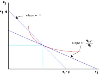
The result that z = 1 is Pareto optimal does not depend on the speci¯c utility function used in the example. In Figure 3 we depict the situation in the (c1; c2) plane. A steady state monetary equilibrium is descirbed by two

properties. First, (c1; c2) must be feasible, so that it must lie on the line

with slope ¡1 through (e1; e2). Second, it must solve the individual's utilty

maximization problem, so that the slope of the indi®erence curve at (c1; c2)

isqt+1=qt. Since qt+1=qt=St+1=Stz = 1=z, the slope of the indi®erence curve

7

More generally, with population growth at rate ° the equilibrium conditions are

ntmt=Mtandnt¿t= (z¡1)Mt. Inserting these into (17), noting thatntSt=qtMt, and

rearranging, we have

St+1=

ze2St

°¯e1¡°(z+¯)St

;

which generalizes (18). Steady state and dynamic monetary equilibria exist if and only if

Figure 3: Optimality of Constant Money Supply

is 1=z. As shown, (c¤

1; c¤2), which is the equilibrium allocation when z = 1,

is Pareto optimal, and wheneverz 6= 1, the equilibrium (c1; c2) is dominated

by (c¤

1; c¤2). Hence, every generation Gt for t¸1 prefers z = 1 to z 6= 1. 8

The next thing to do is to consider a version of the model with storage ¡ that is, to introduce a technology for converting k units of the good at

t into xk units of the good at t+ 1, x > 0. Allowing for the possibility of storage means that agents have more than one way to save. With storage, the budget constraints become

ct1 = e1¡qtmt¡kt (19)

8_{This conclusion holds without alteration or quali¯cation for the case with population}

growth: for any°, equilibrium if Pareto optinal ifz= 1 (andnot_{, as one may have guessed,}

ct2 = e2+qt+1(mt+¿t) +xkt: (20)

We also impose nonnegativity constraints on kt, mt and ctj.

We ¯rst look for nonmonetary equilibria, where qt = 0 for all t. In this case, still using the log-linear utility function, the ¯rst order condition for an interior maximizer kt is

1

e1¡kt

= ¯x

e2+xkt

;

which implies

kt = ¯xe1¡e2 (1 +¯)x ´k

¤_:

Ifx > ¹ =e2=¯e1 then k¤ >0 and the equilibrium involves positive storage;

if x·¹ then storage is 0 and ctj =ej.

We now look for monetary equilibria. A necessary condition for a mon-etary equilibrium to exist is xz · 1. To see this, note that individuals will only hold money if it yields a return at least as great as storage,qt+1=qt¸x;

but this implies St+1=St ¸ xz, and if xz > 1 then St becomes unbounded.

Hence we require xz ·1. Given xz · 1, we now look for a quantity theory equilibrium with kt = 0 and St = S¤_{. As in the case without storage, this}

implies

S¤ ₌ ¯e1¡ze2 z+¯ ,

which is positive if and only if z¹ <1. Hence, for this monetary equilibrium to exist we need two things: z¹ <1, which means that agents want to save, and xz · 1 which means that individuals are willing to save by holding money rather than simply storing goods.9

9_{In addition to the quantity theory equilibrium, when z¹ <1 andxz· 1 there also}

exist monetary equilibria that do not satisfy the quantity equation, although the presence of storage entails di®erent restrictions. In particular, there equilibria where qt+1=qt=x

and agents save in terms of both money and storage at everyt. This impliesSt+1=zxSt,

In terms of welfare, when x > 1 the nonmonetary equilibrium is Pareto optimal and the steady state monetary equilibrium is optimal if it exists (since it only exists if zx · 1, which means z < 1, which is optimal by the argument given for the model without storage). If x · 1, however, equilib-rium with k > 0 is nonoptimal. To see this, note for that any generation such kt >0 it is feasible to increase c1 without decreasing c2 by eliminating

storage and transferring xk from the young to the old at every date there-after. Finally, notice that when z = 1 the monetary equilibrium exists if and only if the nonmonetary equilibrium is nonoptimal.

We now consider some alternative ways to augment the money supply, assuming for simplicity that x = 0 (no storage). The analysis to this point has assumed that new money is given away as a lump sum transfer to the old. An alternative policy is to give old agents transfers that are proportional to their money holdings. In this case, the second period budget constraint is

ct2 =e2+qt+1mtz rather than (15). The ¯rst order condition (for a general

utility function) is ¹=zqt+1=qt, or, by virtue of the equilibrium conditions,

¹(e1 ¡St; e2+St+1) =

St+1

St ; (21)

which should be compared to (16). Notice that z does not appear in (21); therefore the set of equilibrium paths for St (or for any other real variable) does not depend on z under this policy.10

an equilibrium if for all t ¸ 1 we set St+1 = zxSt and set kt to satisfy the ¯rst order

condition

1

e1¡St¡kt

= ¯x

e2+St+1+xkt

:

It is easy to check that total savings,kt+St;di®ers fromk¤unlessz= 1, althoughkt!k¤

as t! 1. Finally, in the borderline case where zx= 1, for anyS02(0; k¤) there is an

equilibrium with St=S0 andkt=k¤¡S0 for allt.

10_{It is sometimes said that monetary policy is \superneutral" if changes in the growth}

Another alternative way to introduce new money is to not give it away but to use it to purchase goods. In this case, the equilibrium condition becomes

¹(e1¡St; e2+

St+1

z ) = St+1

zSt ; (22)

which should be compared to (16) and (21). As long as z¹ < 1, there is a quantity theory equilibrium in which qtmt = S¤ _{and qt=qt+1 = z for all} t. We can use this model to present a simple public ¯nance analysis of the ine±ciency of the in°ation tax relative to lump sum taxation.

As shown in Figure 4, in the quantity theory equilibrium, the real revenue raised by printing money isg, sincect1+ct2 =ct1+ct_¡1;2 =e1+e2¡g. From

the picture, it should be clear that if we set Mt=M0 for all t and raise the

same revenue by lump sum taxes, there is an equilibrium in whichqt=qt+1 = 1

and utility is higher for every generation. Of course, if the government does not have recourse to lump sum taxation, then the optimal mix of distorting taxes may well involve some in°ation; the point here is simply that the in°ation tax is distortionary. The more general point of this section is not only that increasing the money supply may matter, but exactly how one increases it matters a lot.

Finally, to close this section note that the total revenue raised for the gov-ernment by the in°ation tax is a function of the rate of monetary expansion,

g = (z¡1)Mtqt= (z¡1)S. For example, the log-linear utility function can be solved explicitly for S¤ _{= (¯e}

1¡ze2)=(1 +¯), which implies

g = (z¡1)S¤ ₌ (¯e1¡e2)(z¡1)¡e2(z¡1) 2

1 +¯ :

Notice that revenue ¯rst rises and then falls with z, andg = 0 at bothz= 1 and z = ¹z =¯e1=e2. Also, g is maximized at ¹z=2. Hence, we have a classic

\La®er Curve" for the in°ation tax.

Figure 4: The Ine±ciency of the In°ation Tax

1.5

Fiscal Policy

Here we return to nonmonetary economies and consider taxes, transfers and government debt. LetT1 and T2 be time-invariant lump-sum taxes (or

trans-fers if negative) on young and old agents and let g denote government con-sumption. Assuming constant population, for all t, the government budget constraint is given by

T1+T2+±tBt=g+Bt_¡1; (23)

For all t ¸1,Gt maximizes u(ct1; ct2) subject to

ct1 = e1¡T1¡±tbt (24)

ct2 = e2¡T2+bt; (25)

where bt denotes demand for bonds by the young members ofGt. Of course, members of G0 simply consumec02=e2¡T2. If we assume the government

balances the budget every period, then bt = Bt = 0 and T1 = ¡T2 = T

for all t (that is, T is simply transferred from the young to the old). In this case, equilibrium entails ct1 = ej ¡T, ct2 = e2 +T, and ±t = 1=¹,

where ¹=¹(e1 ¡T; e2 +T). By choosing T we can implement any feasible

allocation we want. In particular, if¹(e1; e2)<1 and autarchy is ine±cient,

we can implement the Pareto optimal allocation achieved in the monetary steady state simply by setting T =S¤_.