www.scielo.br/rbg
A CONDUCTIVITY MODEL FOR THE BRAZILIAN EQUATORIAL E-REGION: INITIAL RESULTS
Clezio Marcos Denardini
Recebido em 15 dezembro, 2005 / Aceito em 24 janeiro, 2007 Received on December 15, 2005 / Accepted on January 24, 2007
ABSTRACT.This paper presents results from a new model of field-line-integrated ionospheric conductivity for the Brazilian equatorial region. It was developed aiming to calculate zonal electric fields at E-region heights in the equatorial region. The present model is based on a constant neutral atmosphere model and on an empirical electron densities model (which also gives the ion composition) adjusted by E-region electron density measured by digisonde. It is also based on a geomagnetic field model that we approximate with a dipole which is not located at the centre of the Earth due to the large magnetic declination angle in the Brazilian sector. We have also considered the eccentric dipole having an inclination of 20◦with respect to the Earth rotation axis. The conductivities are calculated for the year 2002 and the results from the present model are compared to those obtained from the conductivity model of the Kyoto University.
Keywords: ionosphere, aeronomy, local conductivity, field aligned conductivity, model.
RESUMO.Este trabalho apresenta os primeiros resultados de um novo modelo para o c´alculo de condutividades integradas ao longo das linhas de campo magn´etico, v´alido na regi˜ao E ionosf´erica do setor brasileiro. Este modelo foi desenvolvido com o objetivo de se calcular os campos el´etricos zonais da regi˜ao E da ionosfera equatorial. Este modelo ´e baseado em um modelo de atmosfera neutra constante e em um modelo emp´ırico de densidades eletrˆonicas (o qual tamb´em fornece a composic¸˜ao iˆonica) corrigido pela densidade eletrˆonica da regi˜ao E medida por digissondas. Devido a grande declinac¸˜ao magn´etica no setor brasileiro o modelo geomagn´etico foi aproximado pelo modelo do dipolo n˜ao centrado com respeito ao centro da Terra. Tamb´em consideramos que o dipolo excˆentrico possui uma inclinac¸˜ao de 20◦com respeito ao eixo de rotac¸˜ao da Terra. As condutividades foram calculadas para o ano de 2002 e os valores resultantes do presente modelo foram comparados com as condutividades obtidas pelo modelo de condutividade da Universidade de Kyoto – Jap˜ao.
Palavras-chave: ionosfera, aeronomia, condutividade local, condutividade alinhada ao campo magn´etico, modelo.
INTRODUCTION
In the equatorial E-region, the partial or total inhibition of the vertical Hall current driven by the primary east-west (dynamo) electric field produces a strong vertical Hall polarization electric field that in turn enhances the equatorial electrojet (EEJ) current (Forbes, 1981). This strong E-region electric field drives plasma instabilities at these heights (Fejer & Kelley, 1980), which pro-pagate westward during day and eastward during night. The pre-sence and characteristics of these irregularities can be monito-red using coherent back-scatter radars (Bowles & Cohen, 1960; Bowles et al., 1960).
Since 1998, the 50 MHz RESCO (a Portuguese acronym for coherent back-scatter radar) radar is operational at S˜ao Lu´ıs (2.3◦S, 44.2◦W, dip:
∼–0.5◦), Brazil. Coherent radars operating
at 50 MHz (λ= 6 m) are sensitive to backscatter from 3-meter plasma irregularities. Radar observation of the EEJ plasma irregu-larities are routinely carried out at S˜ao Lu´ıs. Through this constant monitoring we are able to determine Doppler shifts of the plasma irregularities, among other EEJ information. Since these Doppler shifts are driven by the vertical electric field (Forbes, 1981) this field can be estimated from the radar measurement and, after-wards, the zonal electric field can also be deduced as long as we know the ionospheric conductivity at the E-region height.
Hence, we have developed a geomagnetic field-line-integra-ted ionospheric conductivity model for the Brazilian equatorial re-gion over the radar site, which is presented and discussed here. For validating our results we have calculated the local Hall-to-Pedersen conductivity ratio obtained from this model to com-pare to the same ratio given by the Ionospheric Conductivity Mo-del of the Kyoto University. This moMo-del was chosen mainly be-cause it uses the International Reference Ionosphere Model – IRI Model (Bilitza, 2001) as input for electron density whereas its neutral atmosphere model is based on CIRA 72 model (Rees & Fuller-Rowell, 1988) with the collision frequencies given by Banks & Kockarts (1973). The resulting profiles had shown reasona-ble agreement in the height of peak and magnitude. In the fol-lowing sections we describe the model, the results obtained with and the comparisons with the Kyoto University model.
NEUTRAL ATMOSPHERE, ELECTRON DENSITY AND MAGNETIC FIELD MODELS
We have developed a local ionospheric conductivity model for the Brazilian equatorial E-region based on a constant neutral atmosphere model and on an empirical electron densities mo-del (which also gives the ion composition) adjusted by E-region
electron density measured by a digisonde. It is also based on a geomagnetic field model used to obtain the field line integra-ted conductivities at all heights of radar soundings at the RESCO radar site. The magnetic field model was approximated with a di-pole which is not located at the centre of the Earth due to the large magnetic declination angle in the Brazilian sector. We have also considered the eccentric dipole having an inclination of 20◦with respect to the Earth rotation axis. Based on these inputs the pre-sent model gives the field-line integrated ionospheric conductivi-ties as a function of local time and season.
The above magnetic field line model was chosen because the magnetic equatorial region over Brazil possesses certain peculiarities in the geomagnetic field configuration that are dis-tinctly different from other longitude sectors. A notable peculi-arity is the large magnetic declination angle (being∼21◦W) at
the RESCO radar site. Figure 1 presents a sketch of the magne-tic filed lines (between 89 and 125 km) on the magnemagne-tic meridian corresponding to the magnetic longitude of S˜ao Lu´ıs. The RESCO radar, the magnetic and the geographic equators are also located in this figure.
Figure 1– Sketch of the magnetic filed lines (between 89 and 125 km) on the magnetic meridian corresponding to the magnetic longitude of S˜ao Lu´ıs.
The neutral atmosphere model used as input for the present model is considered to be constituted by the following gases: molecular nitrogen (N2), molecular oxygen (O2), atomic oxygen
atmosphere is assumed to be constituted basically by the ions: nitric oxide (NO+), molecular oxygen (O+
2)and atomic oxygen
(O+). The vertical electron density profiles and the relative ion composition were obtained from the IRI Model (Bilitza, 2001), which is an empirical model based on several available data sour-ces but mainly on digisonde electron density profiles. Abdu et al. (2004) have compared the foE values predicted by IRI with those measured over three locations that formed a conjugated points station pair: Campo Grande in south (20.45◦S, 54.65◦W, dip: –22.5) and Boa Vista in north (02.8◦N, 60.66◦W, dip: 22.5), and an equatorial station, Cachimbo (09.47◦S, 54.83◦W, dip: –3.9). They have found that the daytime equatorial E-layer (foE) is re-asonably well represented by the IRI, but also pointed out that the IRI model underestimates the E-region peak density in the Brazilian sector (se, for example, Figure 4 in Abdu et al., 2004). Thereafter, we have adjusted the absolute electron density given by IRI to the mean electron density obtained from foE at these three stations in 2002. All E-region peak density values obtai-ned from simulations at the dip equator were set to the peak den-sity calculated from the mean foE measured at the correspon-ding local time. The rest of the electron density vertical profile was adjusted proportionally to its previous value considering an
α-Chapman layer decay. For latitudes outside the dip equator, the simulated vertical profiles were corrected by a factor given by the ratio between the peak density obtained from foE and that given by IRI.
Figure 2– Vertical density distributions of the ionospheric constituents (dashed lines), the electron content (continuous line) and the neutral atmospheric cons-tituents (dot-dashed lines).
Figure 2 shows vertical density profiles of the ionospheric constituents, the electron densityNeand the neutral
atmosphe-ric constituents for the equatorial E-region in the Brazilian sec-tor. These profiles, shown here as examples, refer to the southern hemisphere summer at local midday. The continuous line gives
the electron density profile. The dashed lines refer to individuals ionospheric constituents indicated in the graph under the corres-ponding line. And the dot-dashed lines refer to individuals at-mospheric constituents also indicated in the graph in the same way.
RESULTS AND DISCUSSIONS
Using the neutral atmosphere model and the ionospheric model as described above we were able to calculate the collision rates for all latitudes and heights along the magnetic meridian at the longitude of the radar site. The ion-neutral collision rates were calculated as per equation (Kelley, 1989):
νi =
2.6×10⁻⁹
∙(Nn+Ni)∙A−1/2, (1)
whereNnis the neutral atmosphere density,Ni is the ion
den-sity and A = (An+ Ai)is the mean molecular weight
(neu-tral and ionized). Since at the E-region heights the neu(neu-tral den-sity is around 3 to 7 time the magnitude of the ion denden-sity, the term(Nn+Ni)was approximately equal to Nn. In the same
way,Awas approximated to the neutral massAn, so that Eq. (1)
becomes:
νi =
2.6×10⁻⁹∙Nn∙A
−1/2
n . (2)
The electron-neutral collision rates were calculated as per equation (Kelley, 1989):
νe=
5.4×10⁻¹⁰∙Nn∙T
1/2
e , (3)
whereTeis the electron temperature. For the height range used
in the model runs the electron temperature can be approximately equal to the neutral temperature(Tn)without notable effect to the
precision of the model.
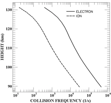
Figure 3 shows examples of the vertical profiles of the col-lision rates calculated by the model using Eqs. (2) and (3). The dashed line represents the ion-neutral collision frequency pro-file, whereas the continuous line is electron-neutral collision fre-quency. Both were calculated for the RESCO radar site coordina-tes, covering the height range of 90 to 130 km, for the equinox period, at 12 h (local time).
Ion(i)and electron(e)cyclotron frequencies were
cal-culated respectively, as per equations:
i =
qe∙B0
mi
and e =
qe∙B0
me
, (4)
whereB0is the geomagnetic field intensity (taken from the IGRF
model),miandmeare the mean ion mass and the electron mass
Figure 3– Vertical profile of the ion-neutral collision rate (dashed line) and ver-tical profile of the electron-neutral (continuous line) calculated for the RESCO radar site location, covering the range height from 90 to 130 km, during equinox, at 12 h (local time).
Making use of these set of equations and the E-region electron densities(Ne)obtained from the IRI model and adjusted in
ac-cordance with what has been described previously, the Hall(σH)
and Pedersen (σP)local conductivities for the RESCO radar
locations were obtained from the usual conductivity equations:
σH = qe2Ne
"
i
mi(νi2+
2
i)
− e
me(νe2+2e)
#
and
σP = qe2Ne
"
νi
mi(νi2+2i)
+ νe
me(νe2+2e)
#
.
(5)
In order to evaluate the present model, the resulting Hall(σH)
and Pedersen (σP)local conductivities were compared to the
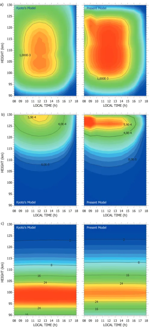
same conductivities obtained by the conductivity model of the Kyoto University, Japan, that is available on internet. These con-ductivities were calculated in both models for the height range of 90 to 130 km between 08 and 18 LT. Figure 4 presents diurnal maps of local Hall conductivity, local Pedersen conductivity, and local Hall-to-Pedersen conductivity ratio for the height range of 90 to 130 km, obtained by the Kyoto University model and the present model. The maps of Hall (Fig. 4a) and Pedersen (Fig. 4b) conductivities reveal that these are higher in the present model than in the Kyoto model. On average, the difference in Hall con-ductivity is∼11%, whereas for the Pedersen conductivity it is ∼15%. These values are very close to the factors used to adjust
the electron density obtained from the IRI model, ranging from 8 to 17%, depending upon the local time.
Since the present model was developed with the aim of cal-culating the equatorial zonal electric fields from the vertical elec-tric field estimated from RESCO coherent radar Doppler velocities of 3-meter plasma irregularities, we have included a comparison between the Hall-to-Pedersen local conductivity ratios obtained from both models (Fig. 4c). Contrary to the previous compa-risons of conductivities, the Hall-to-Pedersen local conductivity ratio is higher in the Kyoto model than in our model. This is not surprising since the Pedersen conductivity from the present model is 15% higher than that of the Kyoto model whereas the Hall conductivity is 11% higher.
There are several reasons which can explain the observed differences. The Kyoto model gives the monthly averaged local conductivities instead of daily values and uses a grid (1◦
×1◦×
1 km) that is larger than the one used in our model (0.5◦×0.5◦× 1 km). Moreover, it is based on the 1990 version of IRI for elec-tron densities, while the present model conductivity relies on the 1995-2000 IRI. In addition, as commented before, the IRI mo-del underestimates the E-region electron densities in the Brazilian sector. With respect to the comparison between the conductivi-ties ratio we attribute the difference to the collision rates used into the present model. We have used the expression of ion-neutron collision frequency given by Chapman (1956), and an update of this equation is needed.
Some others aspects can be also observed in the maps in Figure 4c. An examination of the profiles in these maps reveals that the peak height of Hall-to-Pedersen local conductivity ratio calculated from the present model is located at about 100 km. At this height we have found that the ratio between the conduc-tivities is around 29. This is in very good agreement with the previous results presented by Sugiura & Cain (1966) for 80◦W in the equatorial region. They found that the peak height in near 100 km with the conductivity ratio being∼29, (see, for example,
Fig. 1 of Sugiura & Cain, 1966). The results obtained from the Kyoto model, however, did not coincide either with peak height or with the ratio value. The peak height of the Hall-to-Pedersen local conductivity ratio obtained from the Kyoto model is at about 99 km and the ratio at this height was found to be around 35. These discrepancies are also attributed to the equation used to calculate the collision frequencies as well as to the neutral model chosen.
field(Ez)that drives the EEJ current is mapped along the
mag-netic field lines, its value should also depend on the conducti-vity integrated along the magnetic field line. For this reason we have chosen the approach used by Richmond (1973) on the field line integration. Thus, the present model was designed to cal-culate the Hall(σH)and Pedersen(σP)conductivities at each
point of the geomagnetic field lines along the magnetic meridian at the radar site with height resolution of 1 km, and than integrate them along the geomagnetic field line. Hence, the ratioσH/σP
could be replaced by6H/6Pin the calculations of the electric
fields, now given by:
Ez =
R+θ
−θ σH r∙dθ
R+θ
−θ σP r∙dθ
∙EP ⇒Ez =
6H
6P
∙EP. (6)
Hereris the position vector of the magnetic field line element considering a dipole geometry, θis the magnetic latitude, d θ
is the differential magnetic latitude element vector and the quan-tities6H and6Pare the Hall and Pedersen field-line
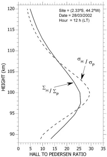
integra-ted conductivities respectively. Figure 5 shows the vertical pro-files of Hall-to-Pedersen conductivity ratio calculated using local conductivities and magnetic field-line integrated conductivities. The Hall-to-Pedersen integrated conductivity ratio was calculated as per equation 6. These profiles were computed for the RESCO radar site location, at local midday during equinox and for high solar activity (SSN>100).
The effect of replacing the termσH/σPby6H/6Pcan be
clearly observed in this figure. The peak height descended by about 2 km and its magnitude decreased from 29 to around 26. An implication of this replacing in the polarization electric field is having its maximum at a lower altitude since it is directly rela-ted to this ration (Eq. 6). Another implication is that the intensity of the polarization electric field should reduce 10 % with respect to that if we have not considered field-line integrated quantities. Also, modification in either Hall or Pedersen conductivities out-side the radar line of sight could change the6H/6P. For
ins-tance, the formation of a sporadic E-layer could change the shape of the electron density profile and then increase the ion-neutral collision frequency (Eq. 1), which in turn would affect slightly different the Hall and the Pedersen conductivities (Eq. 5) chan-ging the Hall-to-Pedersen integrated conductivity ratio and then affecting the polarization electric field.
The mean zonal electric fields obtained from the RESCO coherent radar with the aid of the field-line integrated conducti-vities computed by the present model are shown in the Table 1 (last line) together with several values used in various studies in the past.
Figure 5– Vertical profiles of the local Hall-to-Pedersen conductivity ratio calcu-lated using local conductivities (dashed line) and magnetic field lines integrated conductivities (continuous line).
An examination of this set of published zonal electric fields in comparison with ours indicated that our conductivity model is offering consistent results, because we have obtained zonal electric fields in very good agreement with previous results from similar studies performed in the Indian and Peruvian sector.
CONCLUSIONS
We have developed a simple magnetic field-line integrated con-ductivity model for the Brazilian equatorial E-Region that has pro-duced satisfactory results, but it still has some limitations that if improved could increase its accuracy. First, a limitation arises from the neutral atmosphere model used as input. Here, the neu-tral atmosphere was simplified to an invariant atmosphere made only of four constituents: N2, O2, O and Ar. For a more
Table 1– Zonal electric fields calculated, estimated or assumed at the equatorial E-Region heights from different studies in the Peruvian, Indian and Brazilian Sector.
References Zonal (mV/m) Sector of EEJ study Sugiura & Cain (1966) 2.4 [mean] Peruvian Sector Balsley & Woodman (1971) ∼0.38 –2.06 Peruvian Sector
Balsley (1973) ∼0.1 –0.8 [between 8 and 18 LT] Peruvian Sector Schieldge et al. (1973) ∼0.8 [local midday] Indian Sector
Reddy (1977) 0.3 [assumed] Modeling
Marriott et al. (1979) 1 [typical] Modeling [Peruvian Sector] Viswanathan et al. (1987) ∼0.1 –0,6 [between 8 and 18 LT] Indian Sector
Reddy et al. (1987) ∼0.1 –0.55 [between 8 and 18 LT] Indian Sector
Kelley (1989) ∼0.5 General Present Model in 2002 ∼0.1 –0.4 [between 8 and 18 LT] Brazilian Sector
Comparison of Hall and Pedersen local conductivity obtained with our model and those of the Kyoto model has shown differences around 11% and 15% respectively. The Hall-to-Pedersen local conductivity ratio obtained from the present model, however, was lower than that from the Kyoto model. Also, the height at which the Hall-to-Pedersen local conductivity ratio peaks as calculated from the present model is in very good agreement with the previ-ous results in the literature. When evaluating the Hall-to-Pedersen conductivity ratio obtained from local conductivities compared to that from the magnetic field aligned integrated conductivities we have shown that the height of the peak descend by about 2 km and its amplitude reduces by about 10%. The implication of these changes in the conductivity ratio is on the polarization electric fi-eld which drives the EEJ horizontal current. Considering integra-ted conductivities we expect this electric field to be 10% weaker than that of local conductivities, which subsequently affects in the same way the EEJ current. Finally, a comparison between a set of published zonal electric fields and that calculated with the aid of the field-line integrated conductivities given by the present model reveled a reasonable agreement.
ACKNOWLEDGEMENTS
The author would like to acknowledge Dr. Mangalathayil Ali Abdu who leads the RESCO project and all the colleagues from the RESCO Team for keeping the project going on. This work was partially supported by FAPESP (2005/01113-7).
REFERENCES
ABDU MA, BATISTA IS, REINISCHA BW & CARRASCO AJ. 2004. Equa-torial F-layer heights, evening prereversal electric field, and night E-layer
density in the American sector: IRI validation with observations. Adv. Space Res., 34 (9): 1953–1965.
BALSLEY BB & WOODMAN RF. 1971. Ionospheric Drift Velocity Me-asurements at Jicamarca, Peru (July 1967 – March 1970), World Data Center A – Upper Atmosphere Geophysics, Asheville, North Carolina, USA. pp. 1-45.
BALSLEY BB. 1973. Electric-Fields in Equatorial Ionosphere – Review of Techniques and Measurements. Journal of Atmospheric and Terrestrial Physics, 35(6): 1035–1044.
BANKS PM & KOCKARTS G. 1973. Aeronomy (Part A), Academic Press, London. 430 pp.
BILITZA D. 2001. International Reference Ionosphere 2000. Radio Sci-ence, 36 (2): 261–275.
BOWLES KL & COHEN R. 1960. A Study of the Equatorial Electrojet by Radio Techniques. Journal of Geophysical Research, 65(A8): 2476– 2477.
BOWLES KL, COHEN R, OCHS GR & BALSLEY BB. 1960. Radio Echoes from Field-Aligned Ionization above the Magnetic Equator and Their Resemblance to Auroral Echoes. Journal of Geophysical Research, 65(A6): 1853–1855.
CHAPMAN S. 1956. The electric conductivity in the ionosphere: A re-view. Nuovo Cimento Series 10(Suppl. 4): 1385–1412.
FEJER BG & KELLEY MC. 1980. Ionospheric Irregularities. Reviews of Geophysics, 18(2): 401–454.
FORBES JM. 1981. The Equatorial Electrojet. Reviews of Geophysics, 19(3): 469–504.
HEDIN AE. 1987. MSIS-86 Thermospheric Model. Journal of Geophysi-cal Research, 92(A5): 4649–4662.
KELLEY MC. 1989. The Earth’s Ionosphere. Plasma physics and elec-trodynamics, Academic Press, San Diego, CA. 487 pp.
MARRIOTT RT, RICHMOND AD & VENKATESWARAN SV. 1979. Quiet-Time Equatorial Electrojet and Counter-Electrojet. Journal of Geomagne-tism and Geoelectricity, 31(3): 311–340.
REES D & FULLER-ROWELL TJ. 1988. The CIRA theoretical ther-mosphere model, Advances in Space Research, 8(5-6): 27–106.
REDDY CA, VIKRAMKUMAR BT & VISWANATHAN KS. 1987. Electric-Fields and Currents in the Equatorial Electrojet Deduced from VHF Ra-dar Observations. 1. A Method of Estimating Electric-Fields. Journal of Atmospheric and Terrestrial Physics, 49(2): 183–191.
REDDY CA. 1977. The Equatorial Electrojet and the Associated Plasma Instabilities. Journal of Scientific and Industrial Research, 36(11):
580–589.
RICHMOND AD. 1973. Equatorial Electrojet. 1. Development of a Model Including Winds and Instabilities. Journal of Atmospheric and Terrestrial Physics, 35(6): 1083–1103.
SCHIELDGE JP, VENKATESWARAN SV & RICHMOND AD. 1973. Io-nospheric dynamo and equatorial magnetic variations. Journal of At-mospheric and Terrestrial Physics, 35(6): 1045–1061.
SUGIURA M & CAIN JC. 1966. A Model Equatorial Electrojet. Journal of Geophysical Research, 71(7): 1869–1877.
VISWANATHAN KS, VIKRAMKUMAR BT & REDDY CA. 1987. Electric-Fields and Currents in the Equatorial Electrojet Deduced from VHF Radar Observations. 2. Characteristics of Electric-Fields on Quiet and Distur-bed Days. Journal of Atmospheric and Terrestrial Physics, 49(2): 193– 200.
NOTE ABOUT THE AUTHOR