A workforce size optimization framework for retailers

(1)

A workforce size optimization framework for retailers

Patrícia Gomes da Conceição

Dissertation

Master in Economics

Supervised by

Dalila Martins Fontes Natércia Fortuna

(2)

i

Acknowledgments

I would like to express my sincere gratitude to all the people who contributed to the realization of this dissertation and who accompanied me throughout my academic journey and personal life.

First and foremost, I would like to thank my supervisors Professor Dalila Martins Fontes and Professor Natércia Fortuna, who were always available to help me and who have enriched this work with their exceptional knowledge and valuable advice. I was fortunate to find such good supervisors, and without whom concluding this work would have been more difficult.

To my Master’s tutor, Professor Vítor Carvalho, I thank for his guidance and availability during this academic year.

Also, I want to thank the company NOS Comunicações, S.A., especially the Franchising department, for providing the necessary data to achieve the goals proposed for this dissertation.

I thank my family for all the support, understanding, affection, and motivation they have been giving me throughout my life. Most of all, to my parents, I am eternally grateful for all the sacrifices they have made to invest in my education and for giving me the opportunities that lead to my success. To my sister, I thank her for the patience, useful advice and honest opinions provided in the course of this work.

I thank my closest friends, for always being on my side and for inspiring me to want to do more and better.

Last, but not least, the support of ERDF – European Regional Development Fund through the Operational Programme for Competitiveness and Internationalisation - COMPETE 2020 Programme and the Portuguese funding agency, FCT – Fundação para a Ciência e a Tecnologia within project POCI-01-0145-FEDER-031821 is acknowledge.

(3)

ii

Resumo

A decisão relativa à dimensão da equipa de colaboradores tem vindo a ganhar importância na literatura relativa à gestão do capital humano no sector do retalho, dado o grande impacto que exerce sobre a capacidade e qualidade de atendimento ao cliente, bem como sobre a performance financeira das lojas de retalho. Este trabalho tem como principal objetivo melhorar o processo de planeamento e dimensionamento da equipa de colaboradores, do ponto de vista dos retalhistas, e, consequentemente, diminuir os efeitos nefastos associados a um número insuficiente e/ou excessivo de colaboradores. Para este efeito, sugere-se uma metodologia composta por duas fases que permite obter um número ótimo mensal de colaboradores para uma amostra de lojas franchisadas. Em primeiro lugar, estimou-se um modelo de comportamento das vendas mensais para cada uma das lojas individuais, utilizando dados históricos das vendas, do nível de colaboradores e do tráfego. De seguida, utiliza-se um método iterativo que permite obter o maior número de colaboradores a alocar a cada loja que garante valor acrescentado para a empresa, em termos de acréscimo de vendas. O método proposto é aplicado e validado na empresa de telecomunicações NOS Comunicações, S.A., como caso de estudo. De acordo com os nossos resultados, o número ótimo mensal de colaboradores necessário durante o período em análise (março 2018 – janeiro 2019), é mais elevado do que o número adoptado pela empresa, o que indica que o retalhista tinha um número insuficiente de funcionários. Consequentemente, houve, no referido período, um volume de vendas inferior ao potencial. Mais especificamente, a alocação do número ótimo de colaboradores permitiria um acréscimo de 5% do volume de vendas, face ao realizado.

Códigos JEL: J21; J22; J23; C61

Palavras-chave:

desempenho de vendas; atendimento ao cliente; gestão da equipa de colaboradores; decisão laboral; dados em painel

(4)

iii

Abstract

The staffing level decisions have been gaining importance in retail workforce management literature, given its significant impact on customer service and overall store financial performance. The main objective of this research is to improve the workforce planning process for retailers and consequently diminish the costs associated with both over or understaffed stores and lost sales. For this purpose, a two-stage process that returns an optimal monthly staffing level for a sample of franchised stores is developed. First, a sales response model is estimated for each store, using monthly historical data on sales, actual staffing level, and traffic. Then, an iterative method is used to find the largest staffing level that ensures added value brought to the company in terms of increased sales. The proposed method is applied and validated in the telecommunications company NOS Comunicações, S.A., as a case study. According to our findings, on average the optimal staffing level is higher than the company’s actual staffing level, which suggests that the retailer was understaffing their stores during the period under analysis (March 2018 to January 2019. Adopting the proposed optimal staffing levels would result in a 5% sales lift for the retailer.

JEL codes: J21; J22; J23; C61

Keywords: sales performance; customer service; sales personnel management; staffing

decisions; panel data

(5)

iv

List of Tables

Table 4.1. Description of the variables used in the sales model. ... 21

Table 4.2. Regression results of the sales estimation model. ... 24

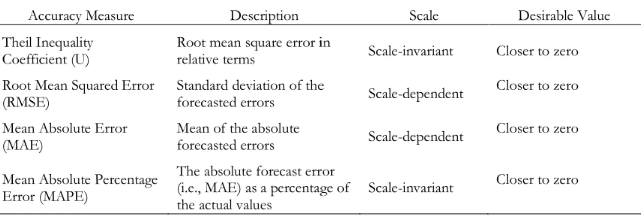
Table 4.3. Description of the forecast accuracy measures used in the model validation. ... 28

Table 4.4. Results of the forecast accuracy metrics. ... 29

Table 4.5. Stores with the highest average labour productivity levels yield by the optimal L... 35

Table 4.6. Frequency of overstaffed, understaffed, and ideally staffed stores. ... 39

List of Figures

Figure 3.1. Flowchart of the iterative procedure used to determine the workforce size. ... 18

Figure 4.1. Geographical distribution of the labour resources and stores throughout the Portuguese districts. The reported values correspond to the number of sales collaborators, and the size of the filled circles represents the number of stores in each district. Data are referring to January 2019. ... 20

Figure 4.2. Comparison of the real and forecasted sales for the store with the (a) highest, (b) lowest, and (c) intermediate total sales volume. ... 27

Figure 4.3. Results obtained under different parameter values for a representative store of the actual staffing level during the test period. Same results for parameter values between 20% and 22%, and from 26% to 30%... 32

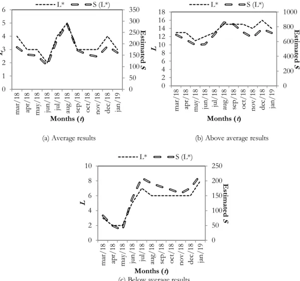
Figure 4.4. Illustrative results of the optimal staffing levels and corresponding sales volume estimate, for an (a) average, (b) above average, and (c) below average store. ... 33

Figure 4.5. Seasonal differences in the staffing requirements: frequency and the most severe cases. ... 34

Figure 4.6. Estimated sales volume with the real and the proposed workforce sizes for the test period along with the percentage sales increase displayed above the two series. ... 36

Figure 4.7. Sales growth evaluation for the stores benefiting the most from our recommendation. ... 37

Figure 4.8. Sales growth evaluation for the stores that were the furthest away from the optimal plan. 38 Figure 4.9. Real and optimal average monthly staffing levels over the period March 2018 – January 2019. ... 39

List of Annexes

Annex A: Descriptive Statistics ... 48

Annex B: Correlation Coefficients ... 49

Annex C: Optimal staffing levels ... 50

(7)

1

1. Introduction

This study introduces and analyses a staffing plan to improve labour planning for retailers. Furthermore, the main objective is to develop a solution approach that allows for determining the monthly workforce size1_{for each store of a retail chain.}

The motivation for this topic arises from a challenge proposed by NOS Comunicações, S.A.2_{, to solve a real personnel assignment problem it faces. Therefore, the validation of} the approach proposed will resort to a comparison between the volume of sales achieved by the determined staffing levels and those of the resulting staffing level of the retailer's current practice.

This particular company is continuously suffering from staff breakdowns, associated with sporadic and structural factors, such as vacations, absences, high traffic peaks, sickness, and exiting from the company. In practice, whenever a store experiences a shortage in sales collaborators, workers from nearby stores are relocated. Although such relocations obviate the understaffing issue, they still lead to negative impacts in the store performance and service quality, since the collaborators brought in is unfamiliar with the working methods of that particular store.

The problem discussed here is not specific to this particular company; evidence suggesting that several retailers have not been making the best labour planning decisions. Thus calling for the need to improve the staffing level decisions. In the hope of saving up on personnel costs, retailers are, in the majority of the cases, understaffing their stores (Chuang, Oliva, & Perdikaki, 2016; Mani, Kesavan, & Swaminathan, 2015; Netessine, Fisher, & Krishnan, 2010; Ton, 2009). This tendency may be related to the fact that retail managers do not consider labour as a source of profits, but rather only as a source of costs. As such, their focus’s on not increasing operational costs, associated with additional staffing (Ton, 2009). So, in order to improve the labour planning decisions, Chuang et al. (2016) advise retailers to make staffing decisions with the aim of maximizing sales and profits, as an alternative to minimizing costs.

1_{Hereafter, we will use workforce size and staffing level indistinguishably.}

2_{Portuguese telecommunications operator, launched in 2014, that provides a full range of communication}

and entertainment services (Internet, telephone, and audiovisual products). NOS is listed in the Portuguese Stock Index (PSI-20) and is one of the most valuable and share turnover companies in the general stock market of the Lisbon exchange.

(8)

2

Ensuring the right staffing level available at a particular store is vital to guarantee successful store financial results, while still maintaining customer satisfaction and loyalty. Verde Group & Baker Retailing Initiative (2007) concluded that the lack of employees was the most frequent complaint amongst 1000 American shoppers that participated in the study, with 6% of customers leaving the store dissatisfied because they were unable to find the assistance they needed.

Therefore, this research is essential for retail management in general, as its outcomes will provide retailers with an efficient solution approach to set in-store labour supply proportional to customer demand; this way improving customer experience while optimizing employee productivity and maximizing sales. So, labour decisions instead of relying solo on sales forecasts, as store managers traditionally do (Fisher, Gallino, & Netessine, 2017; Lam, Vandenbosch, & Pearce, 1998), should take advantage of historical traffic data to determine the most appropriate staffing level.

To some extent, the optimal staffing level, achieved through this framework, can indirectly contribute to some or all of the following: shorter waiting time, higher customer and employee satisfaction, increased customer conversion rate3_{, better work environment,} lower turnover rate, higher volume of sales and profits, and improved store reputation (Quan, 2004).

The rest of this report is organized as follows. Chapter 2 reviews the primary literature concerning workforce planning decisions. In particular, this Chapter focus on the importance of staffing level on the overall retail chain performance (Section 2.1), as well as on the typical process when deploying labour force (Section 2.2). In Chapter 3, the labour planning methodology followed is described, giving some insights into the variables to be used to support this procedure. Chapter 4 presents the case study, giving detailed information regarding the research setting, the data used, uncovering and evaluating the results obtained, and, finally, discussing some of the managerial implications of our findings. Finally, Chapter 5 presents a summary of the main conclusions drawn, as well as some suggestions for future work.

(9)

3

2. Literature Review

Cotten (2007) defines workforce planning as a strategic decision which consists of "ensuring that an organization currently has and will continue to have the right people with the right skills in the right job at the right time performing their assignments efficiently and effectively" (p. 6). Inefficient labour planning decisions in a business organization can be translated into either understaffing, whenever the store labour employed is not enough to meet the customer requirements, or overstaffing whenever an excessive staffing level is available (Ogumeyo, 2010; Quan, 2004).

Particularly in the retail environment, proper labour planning decisions must be a priority for store managers (Ton, 2009), given the great proximity between customers and suppliers which turns employees into a precious resource to deliver exceptional customer experiences and motivate purchase decisions (Prickett, 2018). Also, adequate workforce planning can enhance a retailer’s competitive advantage over competitors (Quan, 2004).

2.1. Importance of staffing level on retail chain performance

Recently, staffing level optimization has been gaining importance in the literature as several papers analyzing the importance of staffing level on customer service and on overall retail store performance have been published (see, e.g., the reviews by Mani et al. (2015) and by Perdikaki, Kesavan, & Swaminathan (2012)).

Using data from forty-one retail stores, Mani et al. (2015) show that short-staffed stores damage retailer's revenue the most, being responsible for a negative impact of 5.74% on store profitability, while overstaffing has a smaller negative impact of 2.04%.

Fisher et al. (2017) studied the impact on revenue by adding labour in a study involving more than 700 stores of a specialized retailer. A positive impact was observed in 168 stores with the following characteristics: "highest potential demand, as indicated by average basket size, several households and household growth, the greatest competition, and the most experienced store managers." (p. 17). According to Ton (2009), the increased profitability is explained directly by a higher conformance quality – capacity of employees to efficiently execute their work - derived by a higher level of staffing. However, concerning flexible labour resources, Kesavan, Staats, & Gilland (2014b) emphasized that this positive relationship does not hold for all staffing levels; when the staffing level reaches a certain saturation point, it is no longer advantageous to increase any further the

(10)

4

level of staffing as it will induce lower sales. As potential causes for this relationship, Heath & Staudenmayer (2000), Raman, DeHoratius, & Ton (2001) and Staats, Milkman, & Fox (2012) claimed the increased distractions, the difficulties in coordinating tasks, and the disturbances in store operations as the staffing level reaches higher numbers.

Some researchers have stressed the importance of having optimal staffing levels by quantifying their benefits in the overall store performance. In particular, Chuang et al. (2016) showed that optimal staffing was responsible for a 10% increase on sales performance in the fashion retail stores analyzed in their study. Mani et al. (2015) estimated store profitability to increase by 3.8% to 5.9% due to an ideal workforce size.

In terms of customer satisfaction, Fisher, Krishnan, & Netessine (2006), Perdikaki et al. (2012), Mani et al. (2015) pointed out the critical role that sales collaborators availability play in the process of converting shoppers into potential buyers. Sales collaborators are facilitators of the purchase process since they can provide the help that customers need, give vital information about a product, find the products more quickly, and even suggest other products that the customer may be interested in. Hence, sub-optimal staffing levels are incapable of answering all the previously stated customer desires, affecting both service quality and customer satisfaction (Mani et al., 2015) negatively. As a result, shoppers begin to lose their trust in the enterprise and eventually start to purchase in a competitor capable of delivering a better service (Chuang et al., 2016). In addition, unhappy customers have the power to generate a harmful word-of-mouth4_{effect by sharing their bad shopping} experiences, which damages the retailer's reputation (Harris & Arendt, 1998). To understand the magnitude of the word-of-mouth effect on consumer behaviour, Verde Group & Baker Retailing Initiative (2007) surveyed 1000 American customers and concluded that 50% of the analyzed sample gave up visiting a particular store because someone else shared a negative experience.

Moreover, inadequate staffing levels can jeopardize employees’ happiness in their work and consequently lead to increased voluntary job turnover5_{(Mosadeghrad, Ferlie, & Rosenberg,} 2011). For instance, whenever a store is understaffed, it is more likely that their employees are over-worked and feeling emotionally stressed, which affects their well-being levels; this way, increasing the incidence of mistakes and poor performance in executing their daily

4_{Transmission of information from person to person by verbal communication.}

(11)

5

tasks (Oliva & Sterman, 2001). On the other hand, highly staffed stores can also affect employee’s motivation to work, since they end up working fewer hours than expected and do not feel as productive as they could be (Thompson, 1998). Besides, retail managers are incurring in higher salary costs in order to pay for those extra-workers, thus affecting their profitability profoundly (Mani et al., 2015).

In brief, both over – and understaffed stores are harmful to the retailer's success, causing lower levels of labour productivity and damaging the retailer’s financial status (Ganster & Dwyer, 1995). To sum up, researchers debating on this topic show a unanimous conclusion that better labour planning has the power of improving retailers' financial performance, while still providing a high-quality service to their customers.

2.2. The retail labour planning process

Usually, the workforce planning procedure comprises two main steps: forecasting staffing requirements and workforce scheduling, based on the amount of labour required and employee availability (Perdikaki et al., 2012).

Next, a more detailed explanation about these steps is presented; however, particular emphasis is given to the first step since it is the one addressed in this research.

2.2.1. Labour requirements forecasting

The determination of the workforce size requires either forecasting sales or traffic, which are reliable indicators of the labour needed to face customer demand (Netessine et al., 2010).

From the literature, it can be seen that two main frameworks are used to determine the staffing requirements, namely: matching labour to sales and matching labour to traffic. The traditional labour practice, which links the sales forecasts with a planned staffing level, is supported by Kabak, Ülengin, Aktaş, Önsel, & Topcu (2008). Also, it is the most commonly used planning method amongst retailers (see, e.g., the retailers used in the studies by Fisher et al. (2006), Kesavan et al. (2014b), and Netessine et al. (2010)).

In the first stage of their optimization framework, Kabak et al. (2008) determined the hourly staffing needs during a workweek based on forecasted sales revenue. The sales forecast was obtained using data on the number of customers, time period (hours), product promotions, and scheduled labour. The relationship between these variables and the

(12)

6

volume of sales is expressed by adopting the store sales function proposed by Lam et al. (1998).

In addition to the sales revenue, past studies also incorporate labour costs in their labour planning decision and set the profit-maximizing staffing levels as the ideal number of sales collaborators, see, e.g., Ahipasaoglu, Erkip, & Karasan (2019), Chapados, Joliveau, L’Ecuyer, & Rousseau (2014), and Mani et al. (2015).

This view is often criticised because it neglects the critical role of traffic on store sales and, thus, fails to transmit to retail managers the real sales potential of their stores (Lam et al., 1998; Netessine et al., 2010; Perdikaki et al., 2012). If the labour planning decisions depend only on actual sales, then the customers who visited the store but did not make any purchase (perhaps due to lack of assistance) are not taken into account (Chuang et al., 2016). Moreover, the strong causal relationship between store labour and sales is an obstacle to the implementation of this method (Fisher et al., 2017; Perdikaki et al., 2012). In contrast, some researchers advocate the traffic-based labour approach as the best way to improve labour planning (Chuang et al., 2016; Lam et al., 1998; Perdikaki et al., 2012). According to Perdikaki et al. (2012), switching from the first framework to the second one lead to an increase of 1.4% in the volume of sales in a large retail chain; in addition, this change is associated with higher customer basket values6_{, thus improving the retailer's} revenue (Netessine et al., 2010). Also, Chuang et al. (2016) have shown, for a specific apparel retailer, that a 10% increase in sales performance is accomplished, merely, by following the proposed traffic approach. The inclusion of a retail foot traffic metric induces a better utilization of workers and makes it easier to identify peak periods, which require greater staff availability (Perdikaki et al., 2012). In contrast to the traditional approach, there is no need to consider the correlation between store traffic and workforce size, since, in the short term, it is unlikely that employee unavailability will have a significant impact in customer flow (Netessine et al., 2010).

Even though few studies have developed a traffic-based method to determine optimal staffing levels. Chuang et al. (2016) proposed a staffing heuristic which uses historical traffic information to determine weekly labour requirements; on the other hand, Lam et al. (1998) relied on traffic forecasts to obtain an appropriate workforce size in a single store.

(13)

7

However, care must be taken when determining labour needs through incoming traffic and a match should be avoided, since not all customer traffic leads to sales. Also, there is heterogeneity between customer traffic behaviour across stores within the same retail chain. Thus, retailers should not use the exact same model to determine labour needs for all stores. Furthermore, Ryski (2005) advises retailers to account for “traffic velocity” (ratio between total traffic and number of operating hours), since the impact of traffic volume depends substantially on store’s working hours.

A drawback of such an approach is the high cost of traffic counters (also known as “customer counters”, “footfall counters” or “people counters”)7_{, which are needed to} obtain accurate traffic information. In addition to the monetary cost, the lack of precision of these devices is another factor discouraging retailers from installing the counters in their stores.

Finally, high traffic peaks may not always be associated with higher productive periods, as customers may be window-shopping and thus, not augmenting store conversion rate, which may render traffic based labour investments unprofitable. Therefore, the usage of a sales-driven labour forecast might be a better choice in order to maximize labour productivity.

2.2.2. Labour scheduling optimization

For Chapados et al. (2014), the computation of the optimal staffing must be followed by a workforce scheduling phase, where retailers allocate those employees to working shifts after accounting for organizational and legal regulations (e.g., working time regulations, rest times, lunch break regulations, and minimum rest period between successive shifts), employees’ skills and preferences, and others (Quan, 2004). Also, Chapados et al. (2014) suggested the inclusion of operational constraints concerning each store, such as store working hours, a mix of full-time and part-time workers, and a minimum staffing level necessary to operate a particular store.

In this allocation process, some authors use pre-existing shifts (see, e.g., Kabak et al., 2008), while others also construct the shifts, i.e., schedules to be assigned to the employees (Chapados et al., 2014; Talarico & Duque, 2015). The most commonly used approach to design staff schedules is mixed integer-programming models, see, e.g., Azmat, Hürlimann,

(14)

8

& Widmer (2004), Corominas, Lusa, & Pastor (2002), and Hertz, Lahrichi, & Widmer (2010).

This research adds up to the scarce literature that takes full advantage of customer traffic data to improve staffing level decisions (Chuang et al., 2016; Kabak et al., 2008; Lam et al., 1998), by proposing and developing a methodology to determine adequate staffing levels (see, e.g., Fisher et al., 2017; Kabak et al., 2008; Tan & Netessine, 2014).

Regardless of some different features, the solution approach presented here is based on the retail labour planning framework proposed by Kabak et al. (2008). However, we add to it by including labour adequacy, measured by the ratio of staffing level to traffic. The labour-to-traffic ratio has been shown to be a determinant factor in determining staffing levels (Chuang et al., 2016). According to them, “what matters is not labour available per se, but how labour compares to traffic" (Chuang et al., 2016; p. 9); thus, its use is expected to improve in-store customer service and prevent overworked employees as this way the employee customer service rate is used. Secondly, we use historical traffic data, rather than traffic forecasting, which is highly volatile (Chuang et al., 2016), Another important improvement is the incorporation of store location factors, such as competitors and buying power, as crucial determinants of the store performance. Nevertheless, most studies on staffing level optimization disregard these factors. Although we do not address the workforce scheduling problem here, essential labour regulations (e.g., the maximum number of working hours allowed by law, and store operating hours) are included in the process of determining an optimal staffing level.

(15)

9

3. Methodology

3.1. Specification of the labour-planning framework

The retail labour-planning framework chosen to improve a retailer’s workforce decision is inspired by that of Kabak et al. (2008) and involves a two-stage process.

The literature reports two main labour-planning approaches, namely: traffic-based approach and sales-based approach. The methodological framework chosen for this study is mainly sales driven, because ultimately, what matters the most for retailers in labour planning is guaranteeing a staffing level that will enhance the store financial results. Explicitly, the staffing decision is based on the forecasted sales volume associated with each staffing level. Furthermore, the workforce size is determined through a sales volume optimization setting that ensures retailers a staffing level that enhances the volume of sales, while minimizing staffing requirements. Even though, the usage of store traffic information has not been completely discarded, as the solution approach proposed here uses historical traffic data to support the staffing decision and highlights the labour-to-traffic ratio as a critical driver of store sales performance. Also, as suggested before, special care is taken to ensure that the model retrieves a staffing level capable of serving the expected customer traffic, based on historical maximum active service.

In the first stage, a sales response model is estimated using monthly historical data from each store of a retail chain; the estimation is performed for each individual store and month. Then, the estimated model is evaluated, through a comparison between the forecasted sales using real staffing levels and the actual sales; naturally, using a different data set. The validation set is vital to ensure that the estimated model appropriately weights all the variables and thus provides a good representation of the store sales measurement. In the case of significant differences between the forecasted and the real data, a recalibration of the model must be done to improve the robustness of the model.

In the second stage, an iterative procedure is used to obtain an optimal monthly workforce size for each store. The main idea behind this method is to keep increasing the staffing level while the added value brought to the retail operation is deemed of interest. The termination criterion chosen requires a particular percentage increase in the volume of sales resulting from a higher staffing level.

(16)

10

Finally, the results obtained by the proposed framework are evaluated through a comparison between the forecasted volume of sales with the staffing level in the second stage and the forecasted volume of sales with the current staffing level. This way, it is possible to check whether the workforce size suggested by the model is capable of delivering higher sales performance for the retailer.

3.1.1. Sales Response Model specification

From the sales estimation models used in previous studies (see, e.g., Kabak et al., 2008; Lam et al., 1998; Mani et al., 2015), the one proposed by Chuang et al. (2016) formulation was chosen, due to the following reasons: introduction of labour-to-traffic ratio (termed labour adequacy) as an explanatory variable, instead of solo relying on labour availability and formulation allowing for the use of panel data8_{. Nevertheless, we extended} Chuang et al. (2016)’ sales function to account for location-specific attributes influencing store sales.

Therefore, in addition to store traffic and labour adequacy, the model proposed here considers the level of competition, purchasing power per capita, and the possession of a mobile service in the store location as explanatory variables of store sales. The inclusion of these additional variables was motivated by previous empirical researches that have studied the influence of some of these factors on the sales performance.

Regarding the competitive factor, an early study by Hise, Kelly, Gable, & McDonald (1983) evaluated the impact of both primary competitors (similar retail stores in the same mall) and secondary competitors (similar departments in stores in the same mall) on the performance of stores located in malls; later on, Arnold, Palmatier, Grewal, & Sharma (2009) examined the influence of store manager behaviours on store performance for different levels of competition; Perdikaki et al. (2012) concluded that the competition environment, used as a control variable in their analysis, adequately explains the store performance; and, finally, Fisher et al. (2017) used it as a store specific attribute and demonstrated that the stores with the most significant competition experience a higher sales increase from additional staffing.

The inclusion of the buying power was inspired by Perdikaki et al. (2012), who investigated the impact of the locations’ per capita income in the stores performance and were able to

8_{Multidimensional data that involves measurements over time for the same group of individuals, units or}

(17)

11

conclude that stores located in neighborhoods with higher per capita income have higher conversion rate.

Lastly, as previous researches suggest (e.g., Cullen, Robinson, Dolphin, Kubitschke, & Clarkin, 1997; McBurney, Parsons, & Green, 2002), defining all potential users of telecommunications services is crucial to forecast the demand for this market; that said, the mobile service rate in the store location was introduced since it reflects the potential customer demand for telecommunications stores, and thus impacts differently their sales performance. From a total of four telecommunications services (Internet, television, mobile, and landline phone), the mobile service was chosen given that it was the service mostly owned by the respondents of a survey carried out by the company used in our work.

Similarly to Chuang et al. (2016), control variables are also included in the regression to capture some time-invariant store characteristics that may affect the outcomes of this study. While these authors controlled individually for store location and store size, this research controls simultaneously both store size and type. Note that store type was also used as a control variable in the study by Luceri, Latusi, Vergura, D. T., & Lugli (2014). Authors other than Chuang et al. (2016) have used store size in their store performance analysis, see, e.g., Hise et al. (1983) and Lusch, Serpkenci, & Orvis (2015).

The monthly fixed effects sales model we propose is given in Equation (1).

𝑺𝒊𝒕 = 𝒆𝜸𝒕𝑵𝒊𝒕

𝜷𝟏_𝒆𝜷𝟐_{𝑳𝑨𝒊𝒕}𝟏 +𝜷𝟑𝑷𝑷𝒊+𝜷𝟒𝑳𝑪𝒊𝒕+𝜷𝟓𝑴𝑺𝒊𝒕+∑𝒋=𝑴,𝑺,𝑮∝𝒋𝑫𝒋𝒊𝑨𝒊+𝝁𝒊𝒕₍₁₎ In summary, our sales response model includes the following variables:

 Sit – sales volume for store i in month t;

 Nit – store traffic for store i in month t;

 LAit – labour adequacy for store i in month t, given by the ratio between the

staffing level (L) and the store traffic (N);

 PPi – purchasing power per capita in the neighborhood of store i;

 LCit – level of competition faced by store i in month t;

(18)

12

 DMi – dummy variable set to one if store i is a shopping mall store, and zero for a

street store, gallery store and citizen store;

 DSi – dummy variable set to one if store i is a street store, and zero for a shopping

mall store, gallery store and citizen store;

 DGi – dummy variable set to one if store i is a gallery store, and zero for a street

store, shopping mall store and citizen store.  Ai – selling area of store i;

 αM,S,G – regression coefficients which represent the response of sales to the selling area of a shopping mall store, street store, and gallery store, respectively, relatively to the same impact exerted by the selling area of a citizen store (reference and omitted category).

 β1,2,3,4,5 – regression coefficients to be estimated;  µit – perturbation term;

 γt – monthly fixed effects estimate.

The relations between the variables implied by the proposed model are validated theoretically and empirically in the literature. Queueing theory9_{suggests that larger staffing} levels (L) are associated with higher sales volume (S) since larger staffing levels lead to a decrease in the waiting time in lines, which turn decreases the number of customers abandoning the store without making any purchase; Chuang et al. (2016) and Hise et al. (1983) sustained this positive relationship empirically. Regarding store traffic, Chuang et al. (2016) evidenced a positive impact on overall sales performance, ceteris paribus.

However, there are diminishing returns to scale associated with these relations, since both staffing level and customer traffic increase sales at a diminishing rate. Indeed, in respect to the former case, several authors claimed that as the store becomes more staffed, each additional collaborator brings a lower positive impact to the sales revenue (see, e.g., theoretical research by Hopp, Iravani, & Yuen (2007) and empirical researches by Fisher et al. (2006), Mani et al. (2015), and Perdikaki et al. (2012)). For the latter case, while Perdikaki et al. (2012) provide empirical evidence of this assumption, in theory, this can be explained

(19)

13

by a larger fraction of customers who are just window-shopping and do not intend to make any purchase and also by the adverse effects of crowded stores on customer purchasing behaviour (Eroglu & Machleit, 1990; Harrell, Hutt, & Anderson, 1980

;

Kesavan et al., 2014a), and having an inadequate staffing level to handle a higher customer demand (Grewal, Baker, Levy, & Voss, 2003). Concerning the crowding effect, it is expected that a higher customer density increases the waiting time in line and deteriorates the customer service, which ultimately can push customers away from making any purchase (Kabak et al., 2008; Perdikaki et al., 2012). Therefore, we anticipate the parameter associated with the store traffic to be positive, but less than 1, that is, 0<𝛽̂<1. As for the sales response to the 1

labour adequacy, we can only anticipate a negative impact, i.e., 𝛽̂ <0, given the results 2

obtained by Chuang et al. (2016).

The purchasing power per capita in the store location will have a positive influence on the sales volume. This prediction is confirmed empirically in the research of Perdikaki et al. (2012), whereas an increase in the location’s per capita income gave rise to higher sales, ceteris paribus.

According to the findings of Hise et al. (1983) and Perdikaki et al. (2012), we expect the level of competition to have a negative impact on the sales volume, i.e., 𝛽̂<0. ₄

Regarding the control variables, following Haans & Gijsbrechts (2011) and Arnold et al. (2009), it is expected that larger stores, of any store type, experience higher sales volumes, i.e., 𝛼̂_𝑀, 𝛼̂, 𝛼_𝑆 ̂_𝐺 >0. In fact, with a larger selling area, sales personnel are capable of serving more customers, the adverse effects of crowding are mitigated, the waiting time in line decreases, and the range of products available to the customers expands; these indirectly lead to a better customer experience, and consequently to a sales improvement.

Finally, as referred to by Cullen et al. (1997) and McBurney et al. (2002), a higher percentage of people owning a mobile service in a given region signals an increase in the demand for closely-located stores offering such services; thereby translating into more sales opportunities. In this context, a positive coefficient is expected for the referred to variable.

Since the sales model given by Equation (1) is non-linear, before applying the different estimation methods, we linearized it by taking the natural log. The log-linearized sales model is given in Equation (2).

(20)

14

ln Sit= γ_t+ β₁ln Nit+β₂_LA1

it+β3PPi+β4LCit+β5MSit+ ∑j=M,S,G∝jDjiAi+μit (2) 3.1.2. Panel data estimation

This section describes and compares the estimation techniques used to obtain the parameter estimates of the log-linearized sales-model. Also, the econometric tests conducted to decide the correct specification for our model are presented.

Initially, the model was estimated without controlling store characteristics and period heterogeneity, i.e., pooled Ordinary Least Squares (OLS) estimation. Then, we applied panel data estimation methods which recognize the panel structure of our data, such as fixed effects (FE) and random effects (RE). Finally, in order to deal with potential endogeneity bias, we used the Generalized Method of Moments (GMM).

The pooled OLS model combines all cross-sectional and time-series data into one dataset, neglecting their differences. If the model does not contain an unobserved effect, then this estimation method is efficient, and the conclusions retrieved by the statistical inference are valid (Park, 2011; Wooldridge, 2010).

However, in the presence of an individual effect (cross-sectional or time-period effect), it’s not recommended to use a pooled OLS regression since its estimation might lead to omitted-variable bias10_{and inconsistent estimators (Wooldridge, 2010). Therefore, in these} cases, the alternative is to use panel data techniques, such as fixed effects and random effects, which include variables to capture the unobserved heterogeneity among different cross-sections. Additionally, the usage of panel data methods is associated with several advantages over the traditional OLS specification, such as higher level of information, more data variation, less collinearity, and more degrees of freedom from combining the two-dimensional information; more adequate models to study the dynamics of change and sophisticated behavioral methods; minimization of the bias of aggregating cases into broader categories; better at identifying and computing the unobserved effects in either cross-section or time-dimension data (Baltagi, 2008; Gujarati, 2009).

In terms of specification, the fixed effects model includes the effects of the individual characteristics as part of the intercept, allowing for each cross-section to have its intercept; whereas the random effects model captures this individual heterogeneity in the error term

10_{Problem of over-estimating or under-estimating the causal effect of the included independent variables,}

which results from the omission of a significant independent variable that is correlated with both dependent variable and one or more other independent variables

(21)

15

(García, 2014). Basically, the main difference between these two models is explained by the properties of the individual effect. The fixed effects approach allows the time-invariant individual effect to be arbitrary correlated with the observed independent variables; while a random effects model considers these differences among individuals to be stochastic and neither correlated with any regressor nor with the idiosyncratic error (Croissant & Millo, 2008).

The Generalized Method of Moments (GMM) technique was performed to account for the potential endogeneity between the staffing level and sales volume (Chuang et al. (2016), Perdikaki et al. (2012), and Mani, Kesavan, & Swaminathan (2011) also use this technique for the same reasons). The endogeneity issue, which translates into biased coefficient estimates, arises due to the following reasons. Firstly, retailers usually decide the staffing level based on the expected demand (sales or traffic); thus, not controlling for expected demand, which may result in biased estimates. Secondly, not incorporating into the estimation procedure the unobserved store characteristics that drive both staffing level and sales volume may lead to biased estimates of the coefficients due to stores unique behaviours. Lastly, the possible dual causality between sales and staffing level may induce the endogeneity bias; in fact, not only the deployed staffing level is able to influence sales, but also the current sales performance can make retailers alter their staffing levels (Lam et al., 1998; Kesavan et al., 2014b).

However, some of the following particularities used in our framework may have mitigated the endogeneity issue: the usage of actual store traffic information, which controls for the expected demand, as suggested by Chuang et al. (2016), Mani et al. (2011), and Perdikaki et al. (2012); and, the inclusion of store size and store type to control for time-invariant store characteristics. Moreover, Chuang et al. (2016) realized through interviews that retailers did not change that often the staffing level decision; this finding might obviate the reverse causal relationship mentioned previously. Nevertheless, we decided to resort to the GMM method to test the robustness of our estimates.

Whenever there is a suspicion that one or more explanatory variables are correlated with the error term of the regression equation, that is, to be endogenous, it is preferable to use the GMM estimation method, which consists of “replacing” the explanatory variable whose exogeneity is dubious by one or more instrumental variables. The instrumental variables need to fulfil two essential conditions: play the same role in the model as the

(22)

16

explanatory variable(s) they are replacing, i.e., should be correlated with the endogenous regressor; and being uncorrelated with the errors (Wooldrige, 2010).

Following Bloom & Van Reenen (2007), Chuang et al. (2016), Kesavan et al. (2014b), Siebert & Zubanov (2010), and Tan & Netessine (2014), we used the lagged values of the staffing level as instrumental variables.

After obtaining the parameter estimates of each model, three statistical tests were conducted to verify the appropriate model for our data. First, the Redundant Fixed Effects Test (or F-test) and the Breusch and Pagan’s (1980) Lagrange Multiplier (LM) test were performed to compare the pooled OLS against the fixed effects and the random effects, respectively. The F-test evaluates the null hypothesis that all time-specific intercepts are equal to zero (pooled OLS), alongside the alternative hypothesis that at least one of those components is not zero (fixed effects). The LM test assesses if the random variance of the individual heterogeneity is equal to zero, which is equivalent to the absence of an unobserved effect. In both tests, the non-rejection of the null-hypotheses indicates that the pooled OLS model is a better specification than the panel data models. If the null hypothesis of the F-test is rejected, then it means that there is a significant fixed effect in our model and thus a fixed effects model is more suitable than a pooled OLS one. On the other hand, the rejection of the null hypothesis of the LM-test suggests that there are substantial differences across cases to be accounted for, thus, favouring a random effects model (Wooldridge, 2010).

Lastly, we performed the Hausman test (Hausman, 1978) to help us decide between the estimates in the fixed effects and random effects models. This test evaluates the null hypothesis of no statistical difference between the two estimates, against the alternative hypothesis of a considerable distance among the models. The similarity between the two estimates happens when both models are consistent, i.e., when individual effects are not correlated with an independent variable. In these situations, it is better to choose the random effects model because it is more efficient than fixed effects. On the other hand, when the estimates statistically deviate from each other it is because one model is consistent and the other is inconsistent; this occurs when the individual effects are correlated with the other regressors, which turns a random effects model inconsistent. Therefore, in these cases, the consistent estimates delivered by a fixed effects model are preferred.

(23)

17

3.1.3. Determination of the workforce size

This section details the iterative procedure used to find an optimal workforce size every month. The baseline of this procedure is the robust sales estimation model obtained in the first stage of the proposed framework.

The flowchart shown in Figure 3.1 illustrates the steps involved in determining the monthly workforce size for each store.

First of all, our framework needs to ensure some minimum staffing levels to sustain the store operation and the customer experience. Therefore, the starting point of this procedure is the minimum staffing level (minl) necessary to (i) have the store open and (ii) satisfy the expected number of customers, based on the historical maximum active service. Details on the computation of this variable are presented later on in this study.

Above the minimum staffing level, the procedure iteratively increases the size of the sales force while the ratio between the estimated sales growth rate and labour growth rate is above a pre-defined threshold (δ); consequently, optimal staffing levels will depend mostly on this threshold. The procedure starts by checking whether the estimated discrete sales growth rate from stage 1 (L=minl) to stage 2 (L=minl+1) is at least δ times higher than the labour growth rate. If that is the case, then the workforce size is incremented by 1 and it proceeds to the next iteration; otherwise, the procedure ends and the workforce size is set to the optimal staffing level. By incorporating the labour growth rate instead of solo relying on the absolute staffing level increase, we have in consideration the current workforce size. As Fisher et al. (2017) point out, the effect of increasing workforce size in the sales volume is expectantly different across stores; thus, this procedure is performed individually for each store (i) and each month (t). This way, we can obtain workforce size recommendations over time for each store, which is the primary purpose of this study.

(24)

18

Figure 3.1. Flowchart of the iterative procedure used to determine the workforce size.

Set L as the optimal staffing level Calculate S(minl) L= L+1 Calculate S(L) L = minl 𝑆 𝐿 − 𝑆 𝐿 − 1 𝑆 𝐿 − 1 Calculate 𝑆 𝐿 − 𝑆 𝐿 − 1 𝑆 𝐿 − 1 ≥ 𝛿𝐿 − 𝐿 − 1 𝐿 − 1 ? No Yes

(25)

19

4. Case Study

4.1. Data

The proposed labour-planning framework was applied in the telecommunications company NOS Comunicações, S.A., as a case study.

4.1.1. Research Setting and Data Collection

NOS Comunicações offers its products and services in physical stores, i.e., retailers, and also through door-to-door sales. The retail service operates through multiple store channels, such as own stores11_{, franchised stores}12_{, and shop-in-shop stores}13_{. Our analysis} was restricted to the franchised stores since these were the stores for which the company requested a labour planning approach and provided the necessary data to test our methodology.

In January 2019, the company had 115 stores operating under a franchising regime. These franchised stores were distributed among five franchisees: Agent A, with 32 stores; Agent B with 27 stores; Agent C, with 25 stores; Agent D, with 31 stores. In total, there were 321 sales collaborators equipping the stores; Agents B and D were the franchisees with the largest and smallest workforce size, respectively. Regarding the geographical distribution of the labour resources, Figure 4.1 shows that they were widely spread over the national territory. It is possible to see that Porto and Braga were the districts with the largest total workforce size; however, this might be associated with the highest store density observed in these locations, that can be observed by the larger circles.

11_{Stores that only sell products and services from the operator, and thus, its sales revenue is wholly directed}

to NOS.

12_{Like own stores, franchised stores sell products exclusively from the principal, i.e., NOS. However, these}

stores are owned by a franchisee agent.

13_{Stores that sell products of any operator, and thus}_,_{the obtained sales revenue is shared amongst the}

(26)

20

Figure 4.1. Geographical distribution of the labour resources and stores throughout the Portuguese

districts. The reported values correspond to the number of sales collaborators, and the size of the filled circles represents the number of stores in each district. Data are referring to January 2019.

Besides, the store chain comprises four different store types: street stores, gallery stores, shopping mall stores, and citizen stores. In January 2019, street stores and shopping mall stores were the most predominant, representing 69% and 17% of the whole store sample, respectively. Gallery stores followed with a smaller percentage of 11% and citizen stores accounted for the remaining 3%.

We obtained the following monthly data from the retailer over the period of March 2017 – January 2019: (i) store sales volume; (ii) staffing level; (iii) store traffic data (i.e., number of customers entering the store and number of open transactions); (iv) adequate service data (i.e., number of customers served and number of closed transactions); (v) location-specific data (i.e., purchasing power per capita, number of competitor stores, and possession of a mobile service); (vi) store size; (vii) store type; (viii) weekly store operating hours (including weekends and excluding lunch breaks)

.

4.1.2. Data Description and Preprocessing

Table 4.1 describes in detail all the variables used in Eq. (1) along with the corresponding data sources.

(27)

21

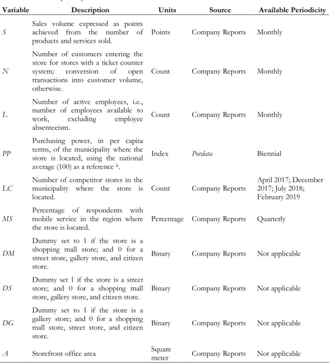
Table 4.1. Description of the variables used in the sales model.

Variable Description Units Source Available Periodicity

S Sales volume expressed as points achieved from the number of

products and services sold. Points Company Reports Monthly

N

Number of customers entering the store for stores with a ticket counter system; conversion of open transactions into customer volume, otherwise.

Count Company Reports Monthly

L

Number of active employees, i.e., number of employees available to work, excluding employee absenteeism.

Count Company Reports Monthly

PP

Purchasing power, in per capita terms, of the municipality where the store is located, using the national average (100) as a reference b_.

Index Pordata Biennial

LC Number of competitor stores in the municipality where the store is

located. Count Company Reports

April 2017; December 2017; July 2018; February 2019

MS Percentage of respondents with mobile service in the region where

the store is located. Percentage Company Reports Quarterly

DM

Dummy set to 1 if the store is a shopping mall store; and 0 for a street store, gallery store, and citizen store.

Binary Company Reports Not applicable

DS Dummy set 1 if the store is a street store; and 0 for a shopping mall

store, gallery store, and citizen store. Binary Company Reports Not applicable

DG

Dummy set to 1 if the store is a gallery store; and 0 for a shopping mall store, street store, and citizen store.

Binary Company Reports Not applicable

A Storefront office area Square _meter Company Reports Not applicable

a _{The percentage of stores with a ticket counter system, and thus for which the real store traffic information was available,} is around 19%. For the other stores, the conversion of open transactions into costumer volume was obtained by resorting to the relationship between the number of customers entering the store and open transactions in the group of stores with the system installed.

b _{This indicator compares the local purchasing power with national performance.} c_{Expect for the last trimester of 2018 and the first trimester of 2019.}

As can be seen in the last column of Table 4.1, not all data were available monthly. Therefore, we had to assume the following period of reference: data from the most up-to-date year, i.e., 2015, as a proxy of the buying power achieved monthly by each municipality; Regarding to the possession of a mobile service (MS), from March 2017 to September 2018

(28)

22

(inclusive), the moment of reference is the correspondent trimester and, from October 2018 to January 2019 (inclusive), it is the 3rd_{trimester of 2018; the monthly level of} competition (LC) refers to the nearest month for which this information was available (for instance, from May 2017 to December 2017, the reference period is December 2017).

While collecting the data, special care had to be taken because of store migration cases to a different franchisee and one consolidation case where two stores have been merged. For the migration cases, we assume the complete store history regardless of the franchise agent to which it belonged; while for the latter case, before the merger, we assume the combined data of the two individual stores, and afterwards, we gathered the consolidated store data.

The time series used, from March 2017 to January 2019, was divided into two subsamples: the fit sample (from March 2017 to February 2018) and the test sample (from March 2018 to January 2019). The fit sample was used to estimate the sales model, in the first stage of our framework, and to compute the maximum active service, required in the second phase. The test sample was used to evaluate the sales estimation model, as an input of the iterative procedure, and, also, to validate the results obtained by our solution approach.

Descriptive statistics of the main variables regarding the complete sample and each subsample are presented in tables 4.7, 4.8, and 4.9, in Annex A. Additionally, pairwise correlations relative to the complete sample and each subsample can be found in tables 4.10, 4.11, and 4.12, in Annex B.

4.2. Results

In this section, the results obtained by the proposed labour planning framework are presented and evaluated. Section 4.2.1 reports the first-stage results, i.e., the sales model regression results and the validation of the calibration obtained. Particular emphasis is given to the second-stage results, in Section 4.2.2, whereas the optimal staffing levels are shown and inferred for a higher sales performance.

4.2.1. First-stage results

Using the unbalanced fit sample(March 2017 – February 2018), we estimate the Pooled OLS; the monthly fixed effects; the monthly fixed effects using the first and eighth

(29)

23

lags of labour as instrumental variables (IV); and the monthly random effects regression models.

4.2.1.1. Estimation results

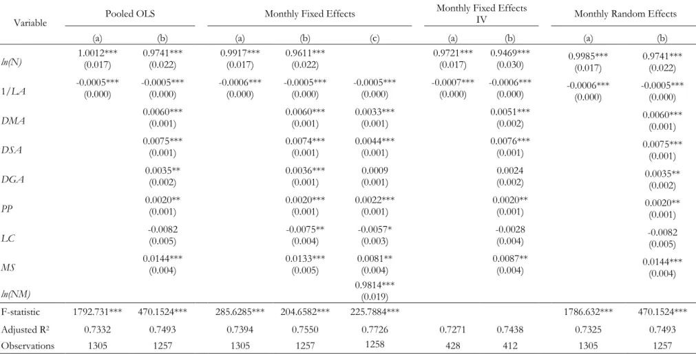
Table 4.2 reports the parameter estimates of the different specifications. Notation (a) shows the estimates of a reduced model accounting only for traffic and labour adequacy as regressors. Notation (b) represents the complete model given in Eq. (2). Notation (c) represents an alternative monthly fixed effects model where we have applied the conversion of open transactions into customer volume for the entire store sample (NM), instead of just using for those stores without the ticket-counter. The figures provided in between brackets are the standard errors for which a consistent estimator for heteroscedasticity and autocorrelation was used.

(30)

24 Table 4.2. Regression results of the sales estimation model.

Variable Pooled OLS Monthly Fixed Effects

Monthly Fixed Effects

IV Monthly Random Effects

(a) (b) (a) (b) (c) (a) (b) (a) (b)

ln(N) 1.0012*** _(0.017) 0.9741*** _(0.022) 0.9917*** _(0.017) 0.9611*** _(0.022) 0.9721*** _(0.017) 0.9469*** _(0.030) 0.9985*** _(0.017) 0.9741*** _(0.022) 1/LA -0.0005*** _(0.000) -0.0005*** _(0.000) -0.0006*** _(0.000) -0.0005*** _(0.000) -0.0005*** _(0.000) -0.0007*** _(0.000) -0.0006*** _(0.000) -0.0006*** _(0.000) -0.0005*** _(0.000) DMA 0.0060*** _(0.001) 0.0060*** _(0.001) 0.0033*** _(0.001) 0.0051*** _(0.002) 0.0060*** _(0.001) DSA 0.0075*** _(0.001) 0.0074*** _(0.001) 0.0044*** _(0.001) 0.0076*** _(0.001) 0.0075*** _(0.001) DGA 0.0035** _(0.002) 0.0036*** _(0.001) _(0.001)0.0009 _(0.002)0.0024 0.0035** _(0.002) PP 0.0020** _(0.001) 0.0020*** _(0.001) 0.0022*** _(0.001) 0.0020** _(0.001) 0.0020** _(0.001) LC -0.0082 _(0.005) -0.0075** _(0.004) -0.0057* _(0.003) -0.0028 _(0.004) -0.0082 _(0.005) MS 0.0144*** _(0.004) 0.0133*** _(0.005) 0.0081** _(0.004) 0.0087** _(0.004) 0.0144*** _(0.004) ln(NM) 0.9814*** _(0.019) F-statistic 1792.731*** 470.1524*** 285.6285*** 204.6582*** 225.7884*** 1786.632*** 470.1524*** Adjusted R2 _0.7332 _0.7493 _0.7394 _0.7550 _0.7726 _0.7271 _0.7438 _0.7325 _0.7493 Observations 1305 1257 1305 1257 1258 428 412 1305 1257

Notes: *, **, *** Significant at 10%, 5% and 1%, respectively. In order to prevent losing information and biased coefficients, stores with some data missing (only in certain

(31)

25

Next, we detailed how the right specification was chosen. In the first place, we decide on the model to use, namely: the fixed effects model or the Pooled OLS regression, through the usage of a Redundant Fixed Effects Test (or F-Test). Given that the p-value obtained was 0.0000, which is lower than 5%, we rejected the null hypothesis and concluded that the fixed effects model is preferred over the Pooled OLS model. In other words, this means that we must incorporate the heterogeneity of each time unit in the estimation procedure. Also, for the purpose of our study, it is advantageous to use a panel data model rather than a simple Pooled OLS estimation, since the latter does not capture the evolution of the store characteristics over time and thus the estimates obtained might not represent accurately the relationships involved in this framework.

Afterwards, we performed a Hausman test to test the fixed effects (FE) model against the random effects (RE) model. With a p-value of 0.0002, we rejected the null hypothesis that the RE model is consistent, and thereby conclude that the FE model was a better fit. Finally, a Hausman endogeneity test was performed to check the staffing level endogeneity, for which two instrumental variables are available: the first and eighth lags of labour. If there is no endogeneity issue, the IV estimates are similar to the FE estimates, and both estimates are consistent. By comparing both estimates, we can infer that instrumentation had a small impact on the FE estimates; thereby, confirming the robustness of our estimates. Even so, the test was performed to draw a more reliable conclusion. The null hypothesis that the staffing level is uncorrelated with the sales volume, i.e., exogenous, was not rejected; this way, eliminating the endogeneity concerns.

In sum, from these tests, we conclude that the FE model, as given in Eq. (2), was the most appropriate for our data and thus, the one to be used in the rest of our analysis, due to the existence of nonrandom individual differences across time over stores. Moreover, the FE model presents a higher adjusted coefficient of determination (adjusted R2_{) than the Pooled} OLS and RE models, which indicates an improvement in the goodness of fit of the model by using this specification.

By comparing the regression results of the FE model in column (a) with those in column (b), it can be seen that the inclusion of more regressors to the original model proposed by Chuang et al. (2016) improved significantly the explanatory power, which is measured by the adjusted R2_{. This confirms that, for our data, the model proposed in this study is more} reliable to explain and predict future sales outcomes. Also, the resulting parameter

(32)

26

estimates from the estimation of the alternative specification, given in column (c), were further apart from our guideline estimation study by Chuang et al. (2016). Although this option would be more consistent, the usage of real traffic data leads to more accurate results; this way, justifying the preference for the estimates considering both direct and indirect measures of customer traffic, which are given in column (b).

As it can be seen, from the FE regression results in Table 4.2, the regression and all independent variables are statistically significant to explain the sales behaviour across stores and across time, i.e., they all exert a significant impact, different from zero, over the sales volume. Besides, these variables explain 75.50% (adjusted R2_{) of the dependent variable,} which is considered to be a significant explanatory power.

Moreover, the estimated parameters have the expected sign, which supports the accuracy of our results. In conformity with Perdikaki et al. (2012), competition influences the sales volume negatively, whereas an increase in one competitor store decreases sales volume by approximately 0.75%, ceteris paribus. As expected, the empirical evidence shows that store traffic, purchasing power per capita, and possession of a mobile service all have a positive impact on the sales volume. Indeed, the positive influence exerted by the store’s location buying power is consistent with the findings of Perdikaki et al. (2012); although the authors have used the location’s per capita income, it can be used as an indicator of the buying power. Although several studies have confirmed that higher store traffic generates more sales (see, e.g., Chuang et al., 2016; Kabak et al., 2008; Perdikaki et al., 2012), our impact is much powerful, reaching almost unitary elasticity; meaning that, the majority of the customers entering in these stores effectively make a purchase.

Regards to the labour adequacy, our result confirms the findings of Chuang et al. (2016); however, in our estimation setting it has a much smaller impact than that of the results reported by Chuang et al. (2016).

In line with Lusch et al. (2015), all the control variables influence the dependent variable positively. Nevertheless, the street store's size accounts for the stronger positive impact upon the volume of sales compared to the effect of the citizen store’s size, our reference category.