Estimating Brazilian monthly GDP: a state-space approach

Estimating Brazilian Monthly GDP: a State-Space

Approach

João Victor Issler

_{Hilton Hostalacio Notini}

July 10, 2015

Abstract

This paper has several original contributions. The …rst is to employ a superior interpolation method that enables toestimate,nowcast and forecast monthly Brazilian GDP for 1980-2012 in an integrated way; see Bernanke, Gertler and Watson (1997, Brookings Papers on Economic Activity). Second, along the spirit of Mariano and Murasawa (2003, Journal of Applied Econometrics), we propose and test a myriad of interpolation models and interpolation auxiliary series – all coincident with GDP from a business-cycle dating point of view. Based on these results, we …nally choose the most appropriate monthly indicator for Brazilian GDP. Third, this monthly GDP estimate is compared to an economic activity indicator widely used by practitioners in Brazil - the Brazilian Economic Activity Index - (IBC-Br). We found that the our monthly GDP tracks economic activity better than IBC-Br. This happens by construction, since our state-space approach imposes the restriction (discipline) that our monthly estimate must add up to the quarterly observed series in any given quarter, which may not hold regarding IBC-Br. Moreover, our method has the advantage to be easily implemented: it only requires conditioning on two observed series for estimation, while estimating IBC-Br requires the availability of hundreds of monthly series. Third, in a nowcasting and forecasting exercise, we illustrate the advantages of our integrated approach. Finally, we compare the chronology of recessions of our monthly estimate with those done elsewhere.

JEL codes: C32,E32, E37

Keywords: GDP Interpolation, State-space Representation, Kalman Filter, Com-posite and Leading Indicators, Nowcasting, Forecasting.

We gratefully acknowledge the comments of participants at CIRET 2008 in Santiago, Chile. We also thank Regis Bonelli and Silvia Matos for allowing us to reproduce the results of their nowcast exercise. All errors are ours. We thank Marcia Waleria Machado, Marcia Marcos, and Rafael Burjack for excellent research assistance and thank CNPq-Brazil, FAPERJ and INCT for …nancial support.

y_{Corrresponding author: Graduate School of Economics – EPGE, Getulio Vargas Foundation, Praia de}

Botafogo 190, s. 1100, Rio de Janeiro, RJ 22250-900, Brazil.

1

Introduction

Any modern society is concerned with its current “state” of economic activity and what should be that state in the near future. Entrepreneurs and individuals are interested in the question because their pro…ts and welfare are a function of it. Governments also have an interest in the subject for budgetary and welfare issues.

For the U.S., the most educated estimate of economic-activity turning points is embodied in the binary variable announced by the NBER Business Cycle Dating Committee: recession vs. expansion for any given month. These announcements are based on the consensus of a panel of experts, and they are made some time (usually six months to one year) after a turning point in the business cycle has occurred. So, today, we only possess old datings for the state of the economy. An alternative to infer business-cycle conditions would be to use Gross Domestic Product (GDP). Indeed, Stock and Watson (1999) argue that, if we were to choose one variable to best represent the state of the economy, this variable would be GDP. They claim that “[...] ‡uctuations in aggregate output are at the core of the business cycle so the cyclical component of real GDP is a useful proxy for the overall business cycle [...]”.

Unfortunately, GDP is also not timely available to continuously infer what is the current state of the economy. First, as far as we know, all countries compute GDP on a quarterly and/or on an annual frequency, but not on a monthly frequency. Second, there are delays in the release of quarterly GDP. Of course, delays vary across countries. In Brazil the delay in the initial release of quarterly GDP is bigger than three months and can reach up to six months at times. Moreover, this initial release is subject to major revisions in six months time.

The fact that a given statistic is only available with some delay does not invalidate its later use for inference if we possess a long-span time-series of it. Indeed, referring to the decisions of the NBER Business Cycle Dating Committee, Issler and Vahid (2006) argue that:

“Suppose that we are asked to construct an index of the health status of a patient. Also, suppose that we know that the best indicator of the health of the patient is the results of a blood test. However, blood samples cannot be taken too frequently, and test results are only available with a lag, sometimes too long to be useful. Our index therefore must be a function of variables such as blood pressure, pulse rate and body temperature that are readily available at regular frequencies. In order to estimate the best way to combine these variables into an index, would we (i) use the historical data on these variables only, or, (ii) use the historical blood test results as well? The answer is, obviously, the latter.”

combining NBER dating information with coincident and leading series of economic activity. Our focus here will be to combine the latter data for Brazil with Brazilian GDP.

As argued above, this strategy can improve our knowledge of GDP in two dimensions. The …rst is that we will possess more frequent business-cycle estimates, i.e., monthly instead of quarterly. This solves an interpolation problem that was proposed by Bernanke, Gertler and Watson (1998) with an econometric model that encompassed most interpolation models that had been previously proposed in the literature; see also the extension in Mönch and Uhlig (2005). The second is that we will be able to nowcast and forecast GDP using information on coincident and leading series of economic activity. This solves a nowcasting problem, to say the least, and has been proposed by Mariano and Murasawa (2003).

The main contributions of this paper are twofold. First, we propose a joint model for Brazilian GDP and Brazilian coincident series that can be used to interpolate and nowcast GDP. Our model is based on the encompassing methods proposed by Bernanke, Gertler and Watson and in Mönch and Uhlig. Second, for forecasting, we will propose an alternative model for Brazilian GDP and Brazilian leading series. It is essentially an extension of the model proposed by Mariano and Murasawa – who are mostly concerned with nowcasting – but will be used for forecasting purposes since we will switch the roles of coincident and leading series in implementing the model. As is clear, our main contribution is empirical, although our motivation to use and combine currently available methods is somewhat original.

In the business-cycle dimension, the ideas and models discussed in this paper are also related to the work of Stock and Watson (1988, 1991, 1993a and b, 2002a and b), Chauvet (1998), Kim and Nelson (1998), Cuche and Hess (2000), Liu and Hall (2001), and Mariano and Murasawa (2010). Regarding the literature on Brazilian business cycles, our paper is related to the work of Contador (1977), Cardoso (1981), Contador and Santos (1987), Nakane (1994), Contador and Ferraz (1999), Spacov (2000), Issler and Spacov (2000), Chauvet (2001, 2002), Picchetti and Toledo (2002), Duarte, Issler and Spacov (2004), Hollauer, Issler and Notini (2009), Central Bank of Brazil (2010), Issler et al. (2012), Issler, Notini and Rodrigues (2013) and Issler, Notini, Rodrigues, and Soares (2013).

The econometric models used for interpolation (also in nowcasting and forecasting) in this paper employ a state-space approach. They have three advantages over other interpolation methods: …rst, they allow the estimation of the unobserved monthly GDP with aggregation consistency, i.e., they ensure that the sum of three-months unobserved GDP data in a give quarter is equal to the respective quarterly observed GDP data. Second it encompasses a wide range of models in the literature – allows di¤erent ways to treat non-stationarity and di¤erent assumptions about the monthly residuals. Third, nowcasting and forecasting are computed imposing the restriction (discipline) that monthly estimates should add up to quarterly observations in-sample, which yields a superior behavior out-of-sample, as our empirical results con…rm.

Finally, with the estimated monthly GDP series on hand, we (re)establish a chronology of recessions of the Brazilian economy, comparing our results with that of the recent literature and with those of the Brazilian Business-Cycle Dating Committee (CODACE). Our turning points are determined using a standard method applied to our interpolated GDP …gures – the Bry and Boschan (1971) algorithm.

the interpolation procedure. In section 4 we present our main empirical results. In section 5 we present a dating chronology for Brazil Business Cycles. Section 6 concludes.

2

State-Space Model and the Kalman Filter for

Inter-polation

2.1

State-Space Representation

In this section, we give a brief review of the use of state-space models and the Kalman …lter. More detailed descriptions can be found in Hamilton (1994) and Harvey (1989). The Kalman …lter provides an e¢cient computational (recursive) mean to estimate the state of a stochastic process – usually put in state-space form. The latter encompasses relationships between observable and non-observable series and a key issue is the estimation of non-observables using past information and/or all information available.

The state-vector representation is given by a system of two vector equations. First, the state or transition equation describes the dynamics of ther 1state vector of possibly

unob-served series t we want to estimate. The second vector equation represents the observation or measurement equation linking the state vector to then 1vector containing the observed series (yt) and possibly some related series(xt)which are either exogenous or pre-determined. Thestate-space representationof the dynamics ofytfort= 1; :::; T ,whereT is the number of observations in our sample, is given by the following system of two vector equations:

t+1 =F t+vt+1 (1)

yt=A0xt+H0 t+wt (2) where F, A0, and H0, are matrices of parameters of dimensions r r, n k, and n r,

respectively. So far, these matrices do not vary across time, but that can be relaxed in a more general setup. Indeed, this will be the case for interpolation, where matrixH will vary

within a given year but is held …xed for any given month across di¤erent years.

Both vector equations have unpredictable error terms1 _{which, for estimation purposes,} are assumed to have a multivariate Normal distribution as follows:

vt

wt

N 0

0 ;

Q 0

0 R : (3)

The coe¢cients matrices F, A0, andH0, and the two variance-covariance matrices Q and R

can be estimated consistently by maximizing the conditional log-likelihood function of the system, given initial conditions 1j0 and on its variance-covariance matrix, labelled P1j0; we

2.2

Filtering and Smoothing

Suppose we observey1; x1; y2; x2; ; yT; xT, but want to estimate the series in the unobserved state-vector t. Denote byItthe information set using the observed seriesy1; x1; y2; x2; ; yt; xt and the conditional forecast of t+1 using information up to t as:

t+1jt =E t+1 It :

Notice that we have assumed that (1) does not depend on xt, which yields:

E( tjxt;It 1) =E( _tj It 1) = _tjt 1: (4)

Also, from (1):

t+1jt=F tjt: (5)

To link that with tjt 1, we note that the structure in (1) and (2) is linear, and recall the

usual structure for updating a linear projections:

tjt= tjt 1+E h

t tjt 1 yt ytjt 1

0i n

Eh yt ytjt 1 yt ytjt 1

0io 1

yt ytjt 1 :

(6) Combining (1) and (6), and using standard formulas for recursive mean-squared error matri-ces, we obtain:

t+1jt = F tjt 1+FE h

t tjt 1 yt ytjt 1

0i n

Eh yt ytjt 1 yt ytjt 1

0io 1 (7)

yt ytjt 1

= F tjt 1+F Ptjt 1H H0Ptjt 1H+R 1

yt ytjt 1 : (8)

Consider now forecastingyt usingxt and past information onIt 1:

ytjt 1 =E(ytjxt;It 1) =A0xt+H0 tjt 1: (9)

Combining (8) and (9) we get:

t+1jt=F tjt 1+F Ptjt 1H H0Ptjt 1H+R 1

yt A0xt H0 tjt 1 : (10)

One can also show that there is a recursion for the variance-covariance matrix Pt+1_jt:

Pt+1jt=F

h

Ptjt 1 Ptjt 1H H0Ptjt 1H+R 1

H0Ptjt 1 i

F0+Q: (11)

The recursive structure in (9), (10) and (11) allows us to state the main results in com-puting Kalman-…lter estimates. First, start the recursion with the unconditional mean and variance-covariance matrix of 1:

1_j0 =E( 1) and P1j0 =E ( 1 E( 1)) ( 1 E( 1))

0

;

and then iterate on (11), (10) and (9) to obtain Pt+1jt, t+1jt and ytjt 1, respectively, for

Suppose we are interested in estimating the unobserved state variable – t. There are two sets of forecasts commonly employed in a Kalman-…lter setup: using the full set of observa-tions available (y1; x1; y2; x2; ; yT; xT), which is called the smoothed estimate of t, or, we can forecast t using only observations available up to periodt 1,(y1; x1; y2; x2; ; yt; xt), which is called the …ltered estimate. Both are presented, respectively, below:

tjT = E( tjy1; x1; ; yT; xT); (12) tjt 1 = E( tjy1; x1; ; yt 1; xt 1): (13)

2.3

Estimation

Under the assumption that the errors vt

wt have a multivariate Normal distribution, i.e., equation (3), consistent and fully-e¢cient estimation of the parameters inF,A0, andH0, and

the two variance-covariance matrices Q and R, can be performed by maximum likelihood.

This assumption implies that the conditional distribution of ytjxt;It 1 is Gaussian as well,

which can then be used to form the sample log-likelihood function with elements ln (ft):

T

X

t=1

ln (ft) = T

X

t=1

ln fytjxt;It 1( ) (14)

=

T

X

t=1

n

2ln (2 ) 1

2ln H

0_P

tjt 1H+R

1

2 yt A

0_x

t H0 tjt 1

0

H0Ptjt 1H+R 1

yt A0xt H0 tjt 1

where fytjxt;It 1( ) denotes the (conditional) density function of ytjxt;It 1, and the

expres-sions for tjt 1 and Ptjt 1 are given in (10) and (11), respectively.

2.4

Nowcasting and Forecasting

Suppose we possess observations ranging from t = 1;2; ; T, and estimate the parameters

in F, A0, and H0, and the two variance-covariance matrices Q and R, by maximizing the

sample log-likelihood (14). As we argued before, there is some delay in making GDP readings available timely and continuously. Thus, when we have the reading for quarterly GDP on T

– comprising the monthsT 2,T 1, andT – calendar time already ranges somewhere from T+3throughT+6, and we already possess coincident-series monthly observations somewhere

fromT+ 1throughT+ 4. So although we refer to this problem asnowcasting because of the status of calendar-time, from an econometric point-of-view this is indeed an out-of-sample forecasting problem with the added twist that we possess already the realizations of the series in xt.

Our starting point is thesmoothed state at the end of the sample: TjT. With, that, using (5), we can then produce:

We are now in a position to forecast yT+1 using the available information on xT+1 and our

previous forecast T+1jT given in (15). From (9):

E(yT+1jxT+1;IT) = A0xT+1+H _T+1jT: (16)

This completes the one-step-ahead forecasts E(yT+1jxT+1;IT) and T+1jT. From then on, we will still have observed x’s to condition on, but our information on y’s will be kept at t =T. The recursive structure in (9), (10) and (11) can then be used to produce nowcasts

for T + 2:

E(yT+2jxT+2;IT) = A0xT+2+H _T+2jT; (17)

T+2jT+1 = F T+1jT +F PT+1jTH H0PT+1jTH+R

1

(18) E(yT+2jxT+2;IT) A0xT+2 H _T+2jT ;

where it should be noted that PT+1jT can be obtained by using (11):

Pt+1jt=F

h

Ptjt 1 Ptjt 1H H0Ptjt 1H+R 1

H0Ptjt 1 i

F0+Q; (19)

which shows that, given the end-of-sample estimatePTjT 1, one obtains immediatelyPT+1jT since we possess estimates of F, H0_{, Q and R. The procedure forT +h, h = 3;4; , etc.,} can replicate that of T + 2, as long as we posses observations on xup untilT +h, whereh is

the number of additional observations we have on x vis-a-vis monthly GDP. This completes

the nowcasting problem.

The truly out-of-sample problem starts when we do not possess anymore observations on the x’s, which occurs after T +h. Here, our proposed strategy is to keep the same

state-space representation given in the previous section, switching only the series in x: in

the nowcasting exercise these essentially are coincident series of economic activity. In the out-of-sample exercise, these will be leading series of economic activity, i.e., series that lead economic activity and therefore are useful for forecasting.

2.5

The Encompassing Model for Interpolation

First, a word of caution about using the term interpolation here. GDP is a ‡ow variable for which we possess quarterly observations we want to distribute within the months in the quarter. Stock and Watson (2010) cite Harvey (1989) to note that the problem of allocating a quarterly ‡ow as such is referred to as distribution, whereasinterpolation estimates monthly values ofstock variables from quarterly values. Despite this technical distinction for‡ow and stock variables, several authors still refer to interpolated GDP, a term that is now ingrained in the literature, being the reason why we employ it here.

Bernanke, Gertler and Watson (1997) proposed a general state-space model that encom-passed several competing models used in the literature for interpolation: Chow and Lin (1971), Fernandez (1981), and Mitchell and Jones (2005), for example. They assume that unobserved monthly GDP (labelled as y+

of the contemporaneous behavior of the interpolated series comes from them. Also in xt are deterministic series such as a constant and/or seasonal dummies. The model proposed for unobserved monthly GDP y+t is:

1 1L pL

p _y+

t = xt +ut

ut = ut 1+"t: (20)

Observed quarterly GDP (labelled as yt here) is the variable being interpolated from quarterly to monthly frequency. It relates to the interpoland series y+t and obeys:

yt =

2 X

i=0

y+

t i, t = 3;6;9;12; : : : T (21)

yt = 0, otherwise. (22)

Hence, quarterly GDP, which we can only observe on months t = 3;6;9;12; : : : T, is the

sum of the corresponding monthly GDPs in that quarter2_{. Otherwise, it is just set to a} …ctional value of zero. Notice that setting yt = 0 for the months we do not observe GDP is a way of making quarterly GDP observable at the monthly frequency; see Mönch and Uhlig (2005), Appendix, just above equation (1). In the Kalman-…lter literature for mixed frequency models (see, for example, Giannone, Reichlin and Small, 2008) a …ctional value is usually assumed for missing observations (zero is the most frequent choice). The crucial step is to impose that the …ctional observed data has a very large variance, so that the zero value is discounted and overwritten by the Kalman-…lter technique. This is exactly how Bernanke, Gertler and Watson and Mönch and Uhlig proceed.

A second issue is how to initialize the values of , , and the variance ofutin the Kalman-…lter procedure. Mönch and Uhlig aggregate the covariates inxt from high (monthly) to low (quarterly) frequency, and run an OLS regression of yt on its lags and xt (regression (20)) at the quarterly frequency. This yields estimates of and the ’s, as well as an estimate for the variance of ut. With the latter, an estimate of is obtained from an OLS regression of

ut on ut 1.

If we assume that the polynomial 1 1L pLp is of order one, i.e.,p= 1, with coe¢cient , our state-space form is the following:

t = 0 B B @ y+ t

y+_t 1

y+t 2

ut 1 C C A= 0 B B @ 0 0 1 0 0 0 0 1 0 0 0 0 0

1 C C A 0 B B @ y+ t 1

y_t+2

yt+3

ut 1 1 C C A+ 0 B B @ xt 0 0 0 1 C C A+ 0 B B @ "t 0 0 "t 1 C C A (23)

yt = H0t t, (24)

2_{Note that the aggregation of monthly GDP can also be made averaging they}+

t ’s, i.e., asyt₌1₃

2 X

i=0 y+t i.

Regardless of how this is done, notice that, up untilT, all estimates of monthly unobserved GDP are obtained

where (23) and (24) are respectively the state and the observation equations and the matrix

H0t is time-varying, with the following format:

H0t =

8 < :

1 1 1 0 ,t = 3;6;9;12; : : : T

0 0 0 0 , otherwise.

(25)

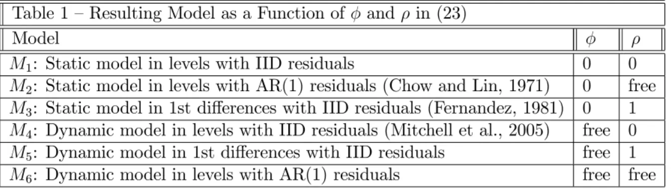
As mentioned before, one interesting characteristic of using the Bernanke, Gertler and Watson approach is that the model described in (23) and (24) encompasses several data interpolation models. They are summarized in Table 1 below. Also, the Appendix contains some discussion of their features and properties:

Table 1 – Resulting Model as a Function of and in (23) Model

M1: Static model in levels with IID residuals 0 0

M2: Static model in levels with AR(1) residuals (Chow and Lin, 1971) 0 free

M3: Static model in 1st di¤erences with IID residuals (Fernandez, 1981) 0 1

M4: Dynamic model in levels with IID residuals (Mitchell et al., 2005) free 0

M5: Dynamic model in 1st di¤erences with IID residuals free 1

M6: Dynamic model in levels with AR(1) residuals free free

2.6

Goodness of Fit Statistics for Interpolated Models

To assess the quality of interpolation, Bernanke, Gertler, and Watson propose the use two

R2 _{measures of …t. Denoting by} d

y+_tjT the smoothed estimate of monthly GDP, and by u_dtjT the same estimate of the error term ut, they consider:

R2_level = VAR d

y+_tjT

VAR yd+

tjT +VAR udtjT

, and,

R2_di¤ = VAR

\_y+

tjT

VAR \y_t+_jT +VAR \utjT

:

Bernanke, Gertler, and Watson claim that it is more informative to report the R2 _{in …rst}

di¤erences since the same statistic in levels will always be close to unity. Thus, we will compute all models listed in Table 1 and compare them regarding their R2_{s, picking the one}

with the best …t.

Given the best models found in empirical tests, all listed in Table 1 above, we can check which of their properties best …t the data: does monthly GDP(yt) follows an autoregressive (AR) process? What does the structure of the monthly residuals look like? In our

3

Empirical Results

3.1

Data

One of the most important factors in the interpolation procedure adopted in this paper is the signal extraction from related series xt. They represent the main information source for interpolation and must ful…ll two requirements:

1. They have to be available in the desired higher frequency of interpolated GDP (monthly in our case) in a timely fashion.

2. They need to have a high correlation with GDP.

The …rst condition imposes a strong restriction for Brazilian data, since there are only a few time-series that cover the entire estimation period (1980-2012) and are available on a monthly frequency. Following Mariano and Murasawa (2003), natural candidates for series in xt would be the coincident series used in business-cycle analysis – Industrial Production, Sales, Income, and Employment. Unfortunately, Income and Employment are only available in Brazil after 2002, since a major change in the Monthly Employment Survey (Pesquisa Mensal do Emprego) made it virtually impossible to chain pre- and post-2002 data. Issler, Notini and Rodrigues (2012) solved this problem by proposing a back-cast algorithm similar to the interpolation method in Bernanke, Gertler and Watson (1997), where pre-2002 data is back-cast on the basis of long-span covariates which are highly correlated with the back-cast series.

Our …rst step is to get as many series as possible that satisfy the …rst condition, later checking which of them satisfy the second condition. As a starting point, we considered the …rst two series that represent monthly economic activity – Industrial Production, labelled IP, and Sales, labelled Sales. For these variables we have long-span data, and they are believed to have cycles that are concurrent with the latent “business cycles.” Since Stock and Watson (1999) argue that, if we were to choose one variable to best represent the state of business cycles, this variable would be the GDP, a natural empirical strategy to interpolate GDP would be to use not only the coincident series used in business-cycle analysis but also additional coincident series as well. The latter can be veri…ed by standard methods – e.g., the Bry and Boschan (1971) algorithm. In order to increase the number of coincident series, we follow Cardoso (1981), from which we have selected additional four candidate series: Energy Demand – labelled Energy, Steel Production – labelled Steel, Cement Production – labelled Cement, and Vehicle Production – labelledVehicles.

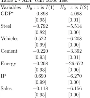
Table 2 - ADF Unit Root Test

Variables H0 :z is I(1) H0 :z is I(2)

GDP 0:898 4:098

[0:95] [0:01]

Steel 0:792 5:514

[0:82] [0:00]

Vehicles 0:522 6:208

[0:99] [0:00]

Cement 0:220 3:392

[0:93] [0:01]

Energy 0:208 26:672

[0:93] [0:00]

IP 0:690 6:270

[0:99] [0:00]

Sales 0:118 6:156

[0:95] [0:00]

Notes: (i) All series are in logs. The speci…cation of the test equation was chosen on the basis of the Schwarz Information Criterion; (ii) the asterisk (*) indicates that a linear trend was included

in the test equation; (iii) …gures in brackets are p-values.

Based on the results of the Augmented Dickey-Fuller (ADF) test in Table 2, we do not reject the null hypothesis that the series areI(1), which makes us conclude that all analyzed

time series have the same integration order of GDP. Next, we apply …rst di¤erences to all these series and compute the correlation between each …rst-di¤erenced series and …rst-di¤erenced GDP, which is reported in Table 33_{. All the analyzed series show a high correlation with the} GDP series once both are …rst-di¤erenced, although the correlation of GDP with Industrial Production and Sales is higher than that of other series. This concludes the cyclical analysis of the auxiliary series4_.

Table 3 - Correlation Coe¢cients – GDP and Coincident Series Variables Cement Vehicles Steel Energy IP Sales GDP 0:49 0:33 0:29 0:21 0:66 0:57

We also investigate the trend pattern between each candidate auxiliary series and GDP. First, we run Johansen’s (1991) cointegration test in order to verify whether there is a long-run relationship between GDP and candidate auxiliary series. As expected, we found that all tested series have one common trend with GDP5_.

Based on the series cycles high correlation and the existence of a cointegration relation-ship, we select Industrial Production and Sales, and possibly Cement Production as well. It 3_{We have to aggregate the monthly series in order to compute correlation coe¢cints. We also compute}

correlations using seasonally adjusted (X12) series. The results are very similar and are available upon request.

4_{We also compute the correlation coe¢cient between each candidate series cycles (extracted by}

Hodrick-Prescott …lter) and GDP cycle. Results are very similar to those in Table 3.

is interesting to note that the traditionally Coincident Series used in business-cycles analysis are the best choices to our interpolation method what con…rms their capacity to track very well the economic activity.

3.2

Evaluation Results

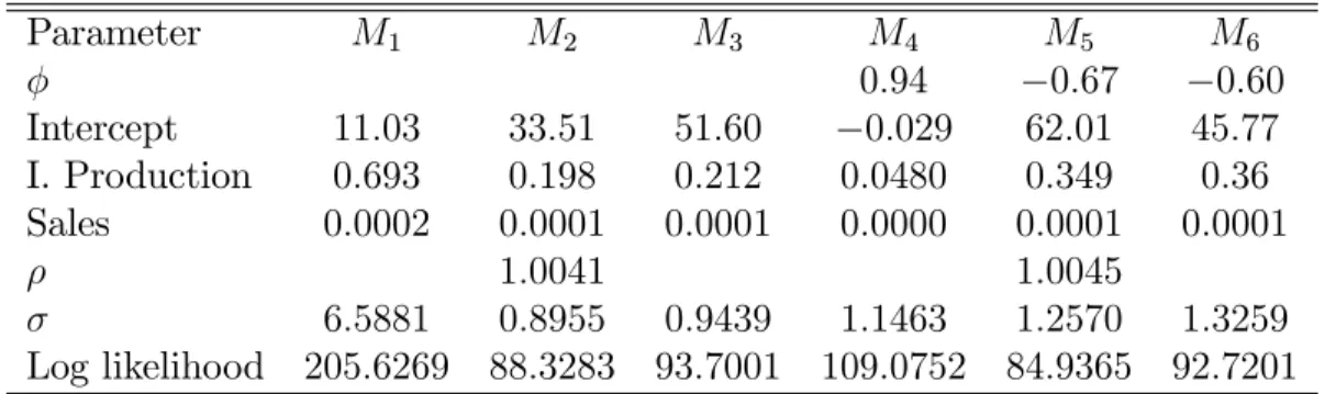
In this section we present the results of the Kalman-…lter estimation for each model consid-ered. Before estimation, all series have been seasonally adjusted using the X12 procedure. In Table 4, we present the estimated parameters and coe¢cients of the auxiliary variables.

Table 4 - Interpolation Results

Parameter M1 M2 M3 M4 M5 M6

0:94 0:67 0:60

Intercept 11:03 33:51 51:60 0:029 62:01 45:77

I. Production 0:693 0:198 0:212 0:0480 0:349 0:36

Sales 0:0002 0:0001 0:0001 0:0000 0:0001 0:0001

1:0041 1:0045

6:5881 0:8955 0:9439 1:1463 1:2570 1:3259

Log likelihood 205:6269 88:3283 93:7001 109:0752 84:9365 92:7201

Notes: (1) The models are described in the text and in the Appendix. (2) Industrial Production and Sales are used as auxiliary series xt.

From the results above we can see that the auxiliary coe¢cients and the estimated pa-rameters change according to the model being estimated. In order to choose the model that best describe our GDP series, we make use of theR2 _{measures of …t to gauge the accuracy of}

interpolation. In Table 5, we present for each model, theR2 _{measures of …t in …rst di¤erence}

for the …ltered and smoothed GDP.

Table 5 -R2

dif f s Measures of Fit Model R2

dif f s (GDP_…ltered) R

2

dif f s (GDP_smoothed)

M1 0:0273 0:0346

M2 0:4652 0:8097

M3 0:4382 0:7923

M4 0:3609 0:7098

M5 0:4011 0:5806

M6 0:3766 0:5736

With the exception of model M1, all models have a high R2, so they show a reasonable

interpolation accuracy. The best R2 _{measures is obtained for Model M}

2, followed by model

M3. Both impose that is zero in (23). They only di¤er about the stochastic process of

the error term: model M2 imposes that the error is an AR(1) process, whereas model M3

imposes that it is an i.i.d. process.

Model M2 is a contemporaneously static model with an AR(1) error term. Taking …rst

an explanatory variables – the so called common-factor model:

(1 L)y+_t = (1 L)xt + (1 L)ut

y+

t = y

+

t 1+xt xt 1+"t;

where"tis white noise and there is an embedded restriction in the dynamic multipliers due to the existence of a common factor. Figure 1 depicts monthly and quarterly GDP, the former being estimated by ModelM2. The …rst graph shows the complete sample (1980-2012) while

in the second one just the recent period (1994-2012). Both show a smooth interpolated series, which …ts closely to the observed quarterly series. Next, we investigate how well interpolated GDP behaves as compared to alternative GDP proxies available in Brazil.

Figure 1 - Monthly (Interpolated) and Quarterly (Observed) GDP

3.3

Comparing and evaluating the monthly GDP with other

eco-nomic activity’s proxies

Monthly GDP estimated in last section could be widely used by practitioners and academics alike interested in measuring in real time the state of the economic activity. It also could be used to detect turning points in the Brazilian economy. In view of that, this section compares our monthly interpolated GDP with an alternative proxy of the economic activity recently constructed by the Central Bank of Brazil - the Brazilian Economic Activity Index - (IBC-Br); see Central Bank of Brazil (2010), for example6_.

IBC-Br is computed by aggregating monthly time-series from economy-wide supply-side sectors: agriculture, industrial sector and services. In agriculture, the source of information is the Systematic Survey of Agricultural Production released by IBGE. Regarding the industrial sector, IBC-Br monthly index is obtained by averaging the indices for four sub-sectors in our National Accounts, which are available on a monthly basis. They are weighted by value added 6_{A detailed methodological description and the complete list of component time series could be found at}

at basic prices of the Quarterly National Accounts System in the previous year. Finally, the services sector includes time series from the trade activities, transportation, storage and mail services, …nancial intermediation, insurance, pension funds and related services, real estate and rentals, management, public health and education and social security, and other services. The …rst advantage of our monthly GDP over IBC-Br is computational. While putting together IBC-Br requires the aggregation of hundreds of monthly series, our interpolation method just requires the use of two covariate series in estimation. Second, IBC-Br method-ology does not impose any restriction (discipline) between estimated levels vis-a-vis that of GDP or between estimated growth rates vis-a-vis that of GDP. In technical language, IBC-Br and GDP need not cointegrate and the cycles in IBC-Br and GDP growth rates need not be synchronized at the quarterly frequency. On the other hand, since our interpolated monthly GDP adds up to quarterly GDP for any given quarter, it must display the same short- and long-run behavior of observed GDP by construction, which is the great advantage of impos-ing discipline at the estimation level. Finally, because our estimate is based on a state-space representation, it can be immediately used to nowcast and forecast GDP7, as discussed in the previous section.

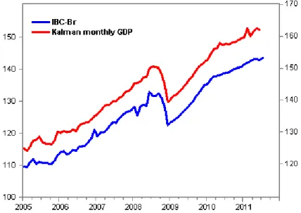
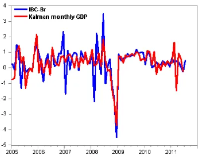
With these points in mind, we now compare these two economic activity proxies. Figure 2 describes both series in levels while in Figure 3 they are depicted in …rst di¤erences. As can be seen, for the period 2005-12, the two series show a very similar trend pattern. However, this is not the case for their growth rates. For the latter, we time-aggregate both proxies of GDP at the quarterly frequency, and then compute their respective quarterly growth rates. These results are plotted in Figure 4. As expected, our estimated GDP proxy growth rate tracks that of quarterly GDP perfectly, which is not true regarding IBC-Br. We observe some larger discrepancies, especially in 2003-05 and 2007-08.

Figure 2 - IBC-Br and Kalman-Filter Monthly GDP (levels)

7_{We should also mention that the IBC-Br series only begins in 2003, which prevents its use in business-cycle}

Figure 3 - IBC-Br and Kalman monthly GDP in …rst di¤erences

Figure 4 - Quarterly Growth Rates of GDP, IBC-Br and Kalman-Filter Monthly GDP

3.4

Detecting Business Cycles Turning Points

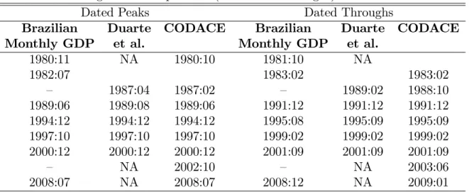
Ta-ble 6 we make turning-point comparisons regarding alternative datings of Brazilian economic activity.

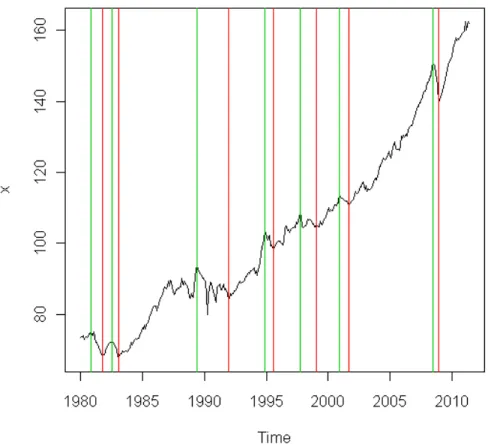
Figure 5 - Monthly GDP - shaded Bry Boshan recessions periods

Table 6 – Turning-Point Comparisons (Peaks and Throughs)

Dated Peaks Dated Throughs

Brazilian Duarte CODACE Brazilian Duarte CODACE

Monthly GDP et al. Monthly GDP et al.

1980:11 NA 1980:10 1981:10 NA

1982:07 1983:02 1983:02

– 1987:04 1987:02 – 1989:02 1988:10 1989:06 1989:08 1989:06 1991:12 1991:12 1991:12 1994:12 1994:12 1994:12 1995:08 1995:09 1995:09 1997:10 1997:10 1997:10 1999:02 1999:02 1999:02 2000:12 2000:12 2000:12 2001:09 2001:09 2001:09 – NA 2002:10 – NA 2003:06 2008:07 NA 2008:07 2008:12 NA 2009:01

Finally, we attempt here a historical account of Brazilian recessions according to our monthly GDP proxy. The recession in 1980-81 can be linked to the increase in interest rates by the FED in the early 1980s, which was later responsible for the emerging-market debt crisis (mostly in Latin America). The 1982-83 recession is related to the Latin American debt crisis itself, where international credit to these economies came to a halt after the Mexican moratorium in 1982. In these two recessions, there was an external factor at work.

Our next dated recession (1989-1991) was “home made,” which came as the result of the Brazilian government inability to curb high in‡ation with many unsuccessful economic plans. These all had in common the absence of long-term …scal discipline, with an initial sudden transitory contraction of money supply.

After the Real Plan, in July 1994, in‡ation …nally gets fairly under control and most re-cessions are again related to events abroad, which generated capital ‡ight and thus prompted a sudden rise in domestic interest rates as a reaction to keep foreign capital in domestic mar-kets. The Mexican crisis in 1994 a¤ected Brazil and other emerging marmar-kets. In 1997-98, the Asian, the Russian, and the Brazilian crises had similar e¤ects here and in other emerging markets. On these occasions domestic interest rates had risen to very high levels, leading to a reduction in domestic economic activity. In 2000-12 our local energy-supply crisis – the ra-tioning of electrical energy for consumers and industry – was responsible to an economy-wide contraction of economic activity, while in 2008-09 we had the global …nancial crisis with a short and limited contraction of Brazilian economic activity.

3.5

Nowcasting GDP

are used to nowcast GDP every month up to one quarter ahead. This quarterly forecast is then compared with the quarterly estimate of IBC-Br – the monthly GDP series put forth by the Central Bank of Brazil (2010) – in terms of its accuracy in forecasting actual quarterly GDP.

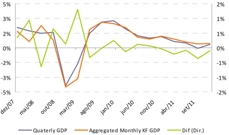
In their exercise, Notini et al. (2012) set the forecasting horizon to be one quarter. Hence, the GDP model forecasts three months ahead in order to nowcast quarterly GDP. Figure 6 contains the results for this exercise, where the green line is the resulting error series transformed to growth rates. As can be seen below, apart from the beginning of 2009, the monthly GDP model nowcasts GDP with high accuracy.

-5% -3% -2% 0% 2% 3% 5% dez/ 07 mai /08 out/ 08 mar /09 ago/ 09 jan/ 10 jun/ 10 nov/ 10 abr/ 11 set/ 11 -2% -1% -1% 0% 1% 1% 2%

Qua terl y GDP Aggrega ted Monthl y KF GDP Di f (Di r.)

Figure 6 - Nowcast Errors of the Monthly GDP Model

Next, we perform an out-of-sample forecast comparison between the monthly GDP model and IBC-Br. Notice that the latter is widely used by the banking industry to nowcast Brazilian GDP. It is important to note that there is no informational gap between our GDP nowcast and that of IBC-Br. So this is a fair nowcasting competition. Notini et al. compute the one-quarter ahead Mean Square Error (MSE) to assess the forecast accuracy of both forecasts. This is computed for two di¤erent periods: 2007:4 to 2011:4 and 2010:4 to 2011:4. Table 6 summarizes the results.

Table 7 - Nowcast Mean Squared Error Monthly GDP Model Versus IBC-Br

Nowcast Period IBC-Br Monthly GDP Model 2007.4 - 2011.4 0.46% 0.40%

2010.4 - 2011.4 0.35% 0.16%

4

Conclusions

In this paper, we propose an estimate for real monthly GDP in Brazil for the period 1980-2012, which is an interpolation of the quarterly observed series; see Bernanke, Gertler and Watson (1997) and Mönch and Uhlig (2005). Our monthly GDP proxy is based on a state-space representation which imposes the restriction (discipline) that the monthly proxy adds up to quarterly observed GDP within every single quarter. A key issue is the choice of covariates used in interpolating the quarterly series: we chose to employ Industrial Production and Sales (corrugated paper sales) as covariates in interpolation, since these two series are key in Brazilian business-cycle analysis; see Duarte, Issler and Spacov (2004) and Issler, Notini and Rodrigues (2012).

The methodology in Bernanke, Gertler and Watson, and Mönch and Uhlig, allows estimat-ing six di¤erent interpolation models, some of which have a long tradition in the literature. We are able to assess the …t of di¤erent models and related series in order to get the most appropriate monthly real GDP estimate: we evaluate six competing models, and six com-peting coincident series (Energy Demand, Steel Production, Cement Production, Vehicles Production, Industrial production and Sales), all available at the monthly frequency for the period 1980-2012.

First, we identify the series which behavior is closer to that of GDP, selecting Industrial Production and Sales. Second, we select the state-space model that has the highest goodness-of-…t statistic vis-a-vis GDP. We chose a contemporaneously static model with an AR(1)

error term – which implies a restricted dynamic structure with one lag of dependent an explanatory variables. This best model is then estimated using Industrial Production and Sales as covariates yielding a smoothed estimate of Brazilian monthly GDP which serves as our GDP monthly proxy.

Next, we perform several interesting empirical exercises: we compare our GDP monthly proxy with alternative proxies available for Brazil. Our main comparison is regarding IBC-Br – the monthly GDP proxy made available by the Central Bank of IBC-Brazil. We discuss the advantages of our approach vis-a-vis theirs; we (re)establish a chronology of recessions in the recent past of the Brazilian economy using our GDP proxy. Its dating of recessions and expansions is compared with those of Duarte, Issler and Spacov (2004) and to those of the Brazilian Business-Cycle Dating Committee (CODACE), showing a close enough dating; we also present the results of an out-of-sample nowcasting exercise using the monthly GDP model. Finally, its forecast accuracy in forecasting actual quarterly GDP is compared with that of the quarterly estimate of IBC-Br. From 2007:4 to 2011:4, its mean-squared error is 13% smaller than that of IBC-Br, whereas, for the recent past, 2010:4 to 2011:4, it is more than 50% smaller, showing its usefulness in nowcasting Brazilian GDP.

References

[1] Bernanke, B. , Gertler, M. and Watson, M. (1997), Systemic monetary policy and the e¤ects of oil price shocks. Brooking Papers on economic activity, (1): 91-157.

[3] Burns, A. F. and W.C. Mitchell (1946), Measuring Business Cycles. New York: National Bureau of Economic Research.

[4] Central Bank of Brazil, 2010, “Índice de Atividade Econômica do Banco Central (IBC-Br),” Relatório de In‡ação de Março de 2010.

[5] Cardoso, E. (1981). “Uma Equação para a Demanda de Moeda no Brasil”. Pesquisa Planejamento Econômico, 11(3), 617-655.

[6] Contador, C. R. and Santos, W. A. C. (1987). “Produto Interno Bruto Trimestral: Bases Metodológicas e Estimativas”. Pesquisa Planejamento Econômico, 17(3), 711-742.

[7] Chauvet, M. (1998). “An Econometric Characterization of Business Cycle Dynamics with Factor Structure and Regime Switching”,International Economic Review, 39, 969-996.

[8] Chauvet, M. (2001) “A monthly indicator of Brazilian GDP”, Brazilian Review of Econo-metrics, v. 21, p. 1-48.

[9] Chauvet, M. (2002), “The Brazilian business cycle and growth cycles”, Revista Brasileira de Economia, v. 56, p. 75-106.

[10] Chow, G. C. and Lin, A. Best linear unbiased interpolation, distribution, and extrap-olation of time series by related series. The Review of economics and statistics, 53(4): 372-375, 1971.

[11] Cuche, N. A. and Hess, M. K. (2000) Estimating monthly GDP in a general Kalman …lter framework: evidence from Switzerland. Economic and Financial Modelling, v. 7, n. 4, p. 153-194.

[12] De Alba, E. (1990). Estimacion del PIB trimestral para México. estudios Económicos 5, 359-370.

[13] Denton, F. T. Adjustment of monthly or quarterly series to annual totals. Journal of the American Statistical Association, 66(333): 99-102,1971.

[14] Duarte, A. M. ; Issler, J. V.; Spacov, A. D. (2004). Indicadores Coincidentes de Ativi-dade Econômica e uma Cronologia de Recessões para o Brasil. Pesquisa e Planejamento Econômico, Rio de Janeiro, v. 34, n. 1, p. 1-37.

[15] Estrella, A. e Mishkin, F. (1999). “Prediciting U.S. Recessions: Financial Variables as Leading Indicators”, Review of Economics and Statistics, 80, 45-61.

[16] Fernandez, R. (1981). ‘A methodological note on the estimation of time series’, Review of Economics and Statistics, vol. 63, pp. 471–8.

[17] Hamilton, J.D. (1994), Time Series Analysis, Princeton: Princeton University Press.

[19] Harvey, A. C. and Pierse, R. G. (1984). ‘Estimating missing observations in economic time series’, Journal of the American Statistical Association, vol. 79, pp. 125–31.

[20] Hollauer, G., Issler, J. and Notini, H. (2009), “Novo Indicador Coincidente para a Ativi-dade Industrial Brasileira”, Revista de Economia Aplicada, v. 13, p. 5-28.

[21] Issler, J. V. and Notini, H. (2008), “Estimating Brazilian Monthly Real GDP: a Kalman Filter Approach”, EPGE, FGV

[22] Issler, J. V., Notini, H., Rodrigues, C. (2013), “Constructing Coincident and Leading Indices of Economic Activity for the Brazilian Economy” Forthcoming in Journal of Business Cycles Measurement and Analysis.

[23] Issler, J.V., Notini, H., Rodrigues, C., and Soares, A. (2013), "Constructing Coincident Indices of Economic Activity for the Latin American Economy" Forthcoming in Revista Brasileira de Economia.

[24] Mitchell T.D., Jones P.D., 2005. “An improved method of constructing a database of monthly climate observations and associated highresolution grids.”International Journal of Climatology, vol. 25, pp. 693–712.

[25] Mariano, R. and Murasawa, Y., 2003, “A NEW COINCIDENT INDEX OF BUSINESS CYCLES BASED ON MONTHLY AND QUARTERLY SERIES,” Journal of Applied Econometrics, 18, pp. 427–443.

[26] Mönch, E. and Uhlig, H. (2005). "Towards a Monthly Business Cycle Chronology for the Euro Area". Journal of Business Cycle Measurement and Analysis 2(1).

[27] Nakane, M.I. (1994). Testes de Exogeneidade Fraca e de Superexogeneidade para a Demanda por Moeda no Brasil. Rio de Janeiro: BNDES.

[28] Notini, Hilton, João Victor Issler, Claudia Rodrigues, Silvia Matos, and Regis Bonelli (2012), “Nowcasting Brazilian monthly GDP: a State-Space approach,” paper presented at CIRET 2012, Vienna. Dowloadable from https://www.ciret.org/…les/vienna_2012_sessionplan.pdf

[29] Stock, J. H. and Watson, M. W. (1988a). "Testing for Common Trends." Journal of the American Statistical Association 83: No. 404 1097-1107.

[30] Stock, J. H. and Watson, M. W. (1988b). "A Probability Model of the Coincident Economic Indicators." NBER Discussion Paper No. 2772.

[31] Stock, J. H. and Watson, M. W. (1989). ‘New indices of coincident and leading economic indicators’, NBER Macroeconomics Annual, pp. 351–94.

[33] Stock, J. H. and Watson, M. W. (1993a). “A Procedure for Predicting Recessions with Leading Indicators: Econometric Issues and Recent Experience”, in New Research on Business Cycles, Indicators and Forecasting, J. Stock e M. Watson, Eds., Chicago: Uni-versity of Chicago Press.

[34] Stock, J. H. and Watson, M. W. (1993b). New Research on Business Cycles, Indicators and Forecasting, J. Stock e M. Watson, Eds., Chicago: University of Chicago Press. [35] Stock, J. H. and Watson, M.W. (2002a). ‘Forecasting using principal components from

a large number of predictors’, Journal of the American Statistical Association, Vol. 97, pp. 1167–1179.

[36] Stock, J. H. and Watson, M.W. (2002b). ‘Macroeconomic forecasting using di¤usion indexes’, Journal of Business & Economic Statistics, Vol. 20, pp. 147–162.

[37] Stock, J. H. and Watson, M.W. (2010). “Research Memoran-dum: distribution of quarterly values of GDP/GDI across months within the quarter.” Mimeo. Princeton University. Downloadable from http://www.princeton.edu/~mwatson/mgdp_gdi/Monthly_GDP_GDI_Sept20.pdf

[38] The Conference Board (1997), “Business Cycle Indicators,” Mimeo, The Conference Board, downloadable from http://www.tcb-indicators.org/bcioverview/bci4.pdf.

A

Appendix

A.1

Detailed Interpolation Models

The literature appoint as the main problem of the models 1a and 1b is the fact that they extract signals only from the presumed stochastic process of the original series in a way that no new information is added. We believe that we would be better o¤ enriching the model with additional information contained in the related series.

Model _M1

This is the simpler model which incorporates information from related series. So it can be used as a benchmark when we estimate the more sophisticated models. It can be stated as:

yt=x0t + t

where: x0_t is a vector of related series and t a iid error term with distribution N(0; 2).

Model _M2

This is the Chow and Lin (1971) model. This model is very used in the literature because they are the …rst to show how to include related series in the interpolation procedure. They suggest a regression model without lagged dependent variables, but autoregressive errors, so we can obtain the Chow and Lin (1971) model by …xing = 0 and by letting to be

"t = 0 B B @ yt

yt 1

yt 2

ut 1 C C A= 0 B B @

0 0 0 1 0 0 0 0 1 0 0 0 0 0

1 C C A 0 B B @

yt 1

yt 2

yt 3

ut 1 1 C C A+ 0 B B @

x0_t

0 0 0 1 C C A+ 0 B B @ t 0 0 t 1 C C A

y+ = h0_t"t

It is important to note that in their seminal paper, Chow and Lin do not use the Kalman …lter but it can be shown that the Kalman …lter above and the Chow and Lin regression yield the same estimates by maximum likelihood (Cuche and Hess).

Model _M3

This is a variation of the Chow and Lin model, suggested by Fernandez (1981), where instead of the regression of yt in levels, it uses the …rst di¤erences of yt in order to account for non-stationarity. This model is obtained by letting regression residuals to be a random walk, i.e. = 0 and = 1.

Model _M4

This model was suggested by Mitchell and Jones (2005) and it is a dynamic version of model M1.

Model _M5

A modi…ed version of model M4 where we impose that = 1.

Model _M6

It is the most general version of the Mitchell and Jones (2005) model, where we let and to be estimated freely.

A.2

Data and Sources

Name

quarterly

monthly

monthly

monthly

monthly

DATA APPENDIX

Variable Frequency Source

(IPEADATA)

GDP IBGE

IGP-DI FGV Índide Geral de Preços

Industrial Production IBGE/PIM-PF Produção Industrial

-Industria Geral

Sales monthly ABPO Expedição de caixas,

acessórios e chapas -papelão ondulado

Energy Demand Eletrobrás Consumo - energia

elétrica

Cement monthly SNIC Produção - Cimento

Vehicles ANFAVEA Produção - Automóveis