UNIVERSIDADE DA BEIRA INTERIOR
Ciências Sociais e Humanas
Economic growth, sustainable development and
food consumption:
Evidence across different income groups of countries
VERSÃO DEFINITIVA APÓS DEFESA
Daniel Francisco Bento Pais
Dissertação para obtenção do Grau de Mestre em
Economia
(2º ciclo de estudos)
Orientador: Professor Doutor António Cardoso Marques
v
Agradecimentos
Gostaria de agradecer ao meu orientador, Professor Doutor António Cardoso Marques pela motivação e produtivas discussões que me proporcionou, especialmente nos momentos mais decisivos. As suas observações, sempre pertinentes, foram uma componente crucial para o aperfeiçoamento deste trabalho.
Queria agradecer também à minha família, pais, irmãos e avós, pelo seu apoio e paciência, especialmente nos últimos momentos onde a tensão era maior, por me escutarem e discutirem algumas das ideias inerentes neste trabalho.
Deixar claro também o apoio dos meus amigos e colegas que de alguma forma proporcionaram igualmente óptimos grupos de discussão e de desanuvio, nos momentos apropriados, pela sua presença sempre que necessária.
Um agradecimento em especial à minha mãe, por todos os pratos vegetarianos que me proporcionou durante os últimos anos, pois sem o seu apoio, a motivação e consequentemente todo trabalho não seriam vistos com o entusiamo que sempre esteve presente.
vii
Resumo
O presente trabalho tem como motivação principal perceber as interações entre o consumo alimentar, crescimento económico e desenvolvimento sustentável. Considerando o elevado crescimento populacional e o acentuado crescimento do rendimento disponível, espera-se que a procura global por alimentos aumente. Não só no sentido de alimentar as populações, mas também de satisfazer uma nova necessidade por produtos densos em calorias e proteínas. Alimentos de pecuária como a carne estão relativamente associados a esta nova tendência, mas também ligados a fortes impactos ambientais e de saúde pública. Perante esta situação, a literatura sugere que o consumo de carne deva ser reduzido pelo benefício do ambiente e da população mundial.
Inspirado por estes factos, este estudo aplica uma análise empírica utilizando uma abordagem ARDL de curto- e longo-prazo, destacando uma análise dividida por 3 níveis de rendimento e recorrendo a um indicador de desenvolvimento sustentável, analisando assim o consumo alimentar, em destaque o consumo de carne maioritariamente abordado na literatura. Para além de abordar também o impacto de uma possível redução no consumo de carne, sugerida na literatura, no crescimento económico e desenvolvimento sustentável.
Após analisar perante diferentes níveis de rendimento e utilizando um indicador de desenvolvimento que considera o impacto ambiental, os resultados sugerem que o consumo de carne, crescimento económico e desenvolvimento sustentável contemplam diferentes relações conforme o nível de rendimento analisado e a perspetiva crescimento/desenvolvimento abordada. Em resumo, o consumo de carne promove o crescimento económico enquanto, por outro lado, prejudica o desenvolvimento sustentável. Evidenciando um dilema entre as duas perspetivas abordadas. Investigação futura é necessária com objetivo de entender quais a soluções mais eficazes, no sentido de não por em causa o crescimento, salvaguardando a componente de desenvolvimento sustentável.
Palavras-chave
Consumo alimentar, crescimento económico, desenvolvimento sustentável, consumo de carne, custos ambientais, abordagem ardl
ix
Resumo alargado
O presente trabalho tem como motivação principal perceber as interações entre o consumo alimentar, crescimento económico e desenvolvimento sustentável. Com base na motivação, as questões centrais da investigação poderão ser apresentadas como: (1) confirmar o efeito positivo do rendimento no consumo de carne, observado na literatura, (2) perceber qual a relação do consumo alimentar, nomeadamente o consumo de carne destacado com maior relevância na literatura, no crescimento económico e no desenvolvimento sustentável, (3) analisar os resultados numa perspetiva de diferentes tipos de rendimento e, por último, (4) compreender qual o impacto da mudança de hábitos alimentares sugerida na literatura. Com a intenção de analisar o impacto do consumo alimentar e a importância do tema em questão, realizou-se uma revisão exaustiva da literatura. Os artigos analisados evidenciam maioritariamente os efeitos do consumo de carne no ambiente através do esgotamento de terra para cultivo e água potável, a deflorestação para plantações de cultivo, os custos das mudanças climáticas associados aos gases efeito de estufa emitidos pelo setor, a perda de biodiversidade, a poluição do ar e da água devido ao uso intensivo de fertilizantes, etc. No seguimento, muitos autores também foram revistos pela sua análise sobre os impactos do consumo de carne associados à saúde pública. O aumento do risco de doenças não transmissíveis, como doenças cardiovasculares e pulmonares, alguns tipos de cancro, diabetes tipo 2, obesidade, entre outros, é associada a hábitos alimentares, principalmente o forte consumo de produtos pecuários, destacando as carnes vermelhas e processadas. Por outro lado, observou-se uma segunda tendência de trabalhos na literatura, especificamente autores que analisam os possíveis impactos de uma redução no consumo de produtos de pecuária e carne. Outros posteriormente discutindo sobre as possíveis abordagens normativas para a sua execução. No entanto, a perspetiva económica encontra-se em falta, e os impactos do consumo alimentar não são considerados nem antes nem após a mudança dietética proposta em benefício do ambiente e da saúde pública. Estes fatores criam a necessidade para a elaboração do presente estudo. Depois de reorganizar a revisão exaustiva da literatura, os dados são abordados e os métodos posteriormente aplicados. Os países utilizados foram os disponíveis e a divisão por grupo de rendimento foi realizada com o objetivo de lidar com a questão da heterogeneidade e entender o impacto em diferentes níveis de rendimento.
Dando início à análise, o impacto do crescimento económico sobre o consumo de carne foi estudado, na medida em que a literatura já explora a relação. O efeito é positivo e, de facto, os níveis de rendimento restringem o consumo de carne, uma vez que um aumento no rendimento provoca um aumento no consumo de carne. Este é o principal motivo, além do
x
crescimento populacional, por detrás da recente tendência do consumo de carne, observado principalmente nas economias emergentes (aqui incluídas como alguns dos países de rendimento médio alto). Além disso, o estudo expande-se, analisando o efeito do consumo alimentar no crescimento económico. O esperado é que o consumo alimentar promova o crescimento económico. No entanto, devido às externalidades associadas ao setor, o efeito no desenvolvimento sustentável poderá não ser tão evidente. Assim, com o objetivo de capturar a perspetiva ambiental, foi aplicado um indicador de desenvolvimento sustentável. O ISEW é conhecido por capturar, para além da económica, as perspetivas sociais e ambientais. A presente análise capta as últimas através das componentes do ISEW, nomeadamente o índice Gini e alguns custos ambientais, em específico associados ao esgotamento de energia, minerais e florestal; e danos causados pelo CO2 no longo-prazo. Uma vez que o setor de alimentos e agrícola estão associados a muitas preocupações ambientais, o ISEW apresenta-se perfeitamente apropriado para a análise.
Uma análise estatística foi realizada antes da análise empírica. Os dados mostram a disparidade dos níveis e taxas de crescimento do consumo de carne nos últimos 50 anos, ao considerar diferentes níveis de rendimento. Nos países mais ricos com altos níveis de consumo de carne é observada uma tendência recente com sinais de diminuição a partir do início do século. As economias emergentes são apresentadas com altos aumentos durante o período analisado, evidenciando a influência das elevadas taxas de crescimento económico. Por fim, as regiões mais pobres não têm mudanças significativas ao longo do período, mantendo o consumo baixo. Os efeitos de curto- e longo-prazo foram realizados aplicando a abordagem Autoregressive
Distributed Lag (ARDL). Seguindo os procedimentos metodológicos habituais para compreender
as características dos dados com o objetivo de realizar a análise mais adequada, concluiu-se que os estimadores Driscoll-Kraay e FE Cluster eram os mais apropriados considerando os fenômenos presentes nos dados. Heterocedasticidade, autocorrelação e cross-sectional
dependence e independence foram observados nos diferentes modelos estudados.
Segundo os resultados. As principais conclusões são que o consumo de carne difere em termos de impacto ao considerar diferentes níveis de rendimento. Os países mais ricos que importam carne de regiões mais pobres e mais baratas são afetados negativamente em termos de PIB. Mas, enquanto os alimentos não são produzidos no país, as regiões mais ricas deslocam os custos ambientais para os exportadores. Por outro lado, os países que produzem e exportam beneficiam em termos económicos, embora negligenciando os custos ambientais não capturados pelo PIB, mas significativos no ISEW. No entanto, a falta de qualidade nos dados dos países mais pobres poderá estar a afetar os resultados desse grupo. Em geral, o consumo de carne introduz um dilema. Seja para produzir, sem considerar os custos ambientais, ou considerar uma abordagem mais sustentável, preservando os ecossistemas, mas reduzindo as taxas de crescimento económico. Soluções são necessárias para uma estratégia win-win.
xi
Abstract
The major motivation behind the present study is to analyze the interactions between food consumption, economic growth and sustainable development. Considering that high population and income growths will lead the coming decades, an increase in global food demand is expected. Not only in terms of feeding the population but also to satisfy their recent needs of more calorie- and protein-dense foods. Livestock products such a meat are closely related to this trend, but also associated with impacts on the environment and public health. From land and water depletion, to greenhouse gases emissions and higher risks of non-communicable diseases. Therefore, an answer to this problem is needed. The literature suggests that meat consumption should be reduced for the sake of the environment and global population
Inspired by these facts, this study employs an empirical approach, analyzing through three income groups and applying a sustainable development indicator, analyze the interactions of food consumption, specially meat consumption as the literature highlights. And the impact on the economy of a possible reduction in meat consumption suggested by the literature.
By analyzing for different income groups and using a sustainable development indicator, our findings suggest that meat consumption, economic growth and sustainable development have different relationships considering income level. Succinctly, meat consumption promotes economic growth following the GDP, but neglects the sustainable development ISEW. Evidencing a dilemma between economic growth and economic sustainability. Further research is needed with the objective of further understand which solutions are more effective, as with the intent to promote growth, while considering the environmental perspective.
Keywords
Food consumption, economic growth, sustainable development, meat consumption, environmental costs, ardl approach
xiii
Index
1. Introduction ... 1
2. Literature Review ... 3
2.1. The Environmental Costs of the Agricultural/Food Industry ... 3
2.2. The Public Health Risks associated with Food consumption ... 5
2.3. Food and economic growth ... 6
2.3.1. Food (in)efficiency ... 6
2.3.2. Income and meat consumption ... 7
3. Methodology ... 8
3.1. Data ... 8
3.2. Descriptive Statistics ... 11
3.3. Methods... 15
4. Empirical Results ... 18
4.1. Does income promote meat consumption? ... 19
4.2. The influence of sustainable development (ISEW) on meat consumption ... 20
4.3. Could meat consumption be an economic growth driver? ... 21
4.4. Meat consumption impact on sustainable development ... 23
5. Discussion: food, the output approaches and the wealth of the countries ... 24
5.1. Economic growth promotes meat, while sustainable development slows it ... 25
5.2. Meat: the growth and sustainable approaches dilemma ... 27
6. Conclusion and final remarks ... 31
7. References ... 33
xiv
List of Figures
Fig. 1. Evolution of meat consumption in 3 countries of each income group, period 1961-2013 Fig. 2. Relationship between meat consumption and income per capita for all countries Fig. 3. Relationship between income per capita and meat consumption for all countries
xv
List of Tables
Table 1. ISEW type of components, variables, sign, calculus and data sources for all countries Table 2. Specification tests
Table 3. Specification tests (cont.)
Table 4. Semi-elasticities, elasticities and adjustment speed for MC with GDP, using FE Cluster Table 5. Semi-elasticities, elasticities and adjustment speed for MC with ISEW, using FE Cluster Table 6. Semi-elasticities, elasticities and adjustment speed for GDP, using DK-FE
Table 7. Semi-elasticities, elasticities and adjustment speed for ISEW, using DK-FE Table 8. Synthesis of results for meat consumption following both approaches Table 9. Synthesis results of both approaches following meat consumption Table A.1. Models notation and specification
Table A.2. Descriptive statistics and cross-sectional dependence for HIC Table A.3. Descriptive statistics and cross-sectional dependence for UMIC Table A.4. Descriptive statistics and cross-sectional dependence for MLIC Table A.5. Variables definition, sources and models where applied Table A.6. Results of the 2nd generation panel unit root test CIPS Table A.7. Results for MC analysis with GDP, using FE Cluster Table A.8. Results for MC analysis with ISEW, using FE Cluster Table A.9. Results for GDP analysis, using DK-FE
xvi
List of Acronyms
ARDL Autoregressive Distributed Lag
CIPS Cross-Sectional Augmented Panel Unit Root Test DK Driscoll-Kraay Standard Errors
ECT Error Correction Term
FE Fixed Effects
FSP Food Security, Protein GDP Gross Domestic Product HIC High-Income Countries
ISEW Index of Sustainable Economic Welfare
MC Meat Consumption
MLIC Middle Lower-Income Countries PBC Plant-based Consumption UMIC Upper Middle-Income Countries VIF Variance Inflation Factor XNI Exports/Imports Index
1
1. Introduction
Some authors predict that by 2050 the world population will reach 9.7 billion (United Nations, 2017), contributing to almost 3 billion more mouths to feed. Not only that but, alongside it, worldwide wealth has been increasing for the past decades, especially both in emerging economies and developing countries. Combining these two aspects, population and wealth high growth rates, a serious shift in dietary habits is expected. Meat consumption has been a prioritized option when choosing what to eat, due mainly for its affordability and accessibility, and its nutrition value, a source of protein and B-complex vitamins. Despite the past growth, high-income countries (HIC) have halted the consumption of meat and its by-products and even reducing it as observed recently, however reaching at high levels, two to three times the world average. Moreover, emerging and developing economies are observed to be shifting their dietary habits through benchmarking the same animal-based calorie-heavy diets followed in the developed world. According to Vranken et al. 2014 world meat production has increased from 65 to 279 million tons in the last 50 years, an increase of more than 400%. This would not be a concern if the consumption of livestock products were not associated with a complex spectrum of contemporary issues. From the environmental perspective to public health and even food security.
Studies from different scientific areas have highlighted the relationships livestock production and consumption have on the environment through natural resources depletion, mainly land and water, environmental degradation, mostly in form of deforestation and loss of biodiversity, and the emissions associated with the sector. On the other hand, livestock, and mainly processed and red meats, have been associated with higher risks of non-communicable diseases (NCD), such as cardiovascular, some cancers, type 2 diabetes and obesity, as well with higher resistance rates from humans to antibiotics. Food security is also questioned in the way that the conversion of plant-based crops, used to feed livestock, for meat is debatable and considered by some authors inefficient, compared to other types of foods.
Although livestock products remain an important contribute to the subsistence of our contemporary societies for its nutrition properties, affordability and accessibility and, in part, for the culture rooted in our civilizations, as well as a source of income, as a consequence of its consumption, plant-based products are associated with several advantages, such as reduced greenhouse gases emissions (GHGEs) and natural resources depletion or contribute to a healthier life, with lower risks of NCDs. Due to globalization and an easier access to information, knowledge on the impact of certain consumptions have recently drawn fresh questions into the debate of sustainable living. And various targets and policies have been implemented in form of economic, social and legal instruments with the aim of meeting the commitment for more sustainable habits (Abadie et al. 2016; Leach et al., 2016; Lombardini & Lankoski, 2013).
2
While most of the studies have analyzed the impact of a diet change, mainly from a meat- to a plant-based, on the environment and health, it seems that a gap exists in linking such a change with the whole economy. As such, the objective of this study is to analyze the interactions between food consumption, economic growth and sustainable development. The literature already highlights the benefits of restricting meat consumption followed by an increase in plant-based foods consumption, but to promote such a shift it is crucial to understand the effects on a wider perspective and be sure that such a structural change in the rooted dietary habits of the population do not threat the economic growth and sustainable development of a country.
Before the empirical analysis, an exhaustive literature review was made to understand the impacts of meat consumption mainly on the environment and public health. The analysis of the effects of income on meat consumption was also observed in the literature and thus compared with the results of the present study. The empirical analysis is focused on a set of 78 worldwide countries divided into three groups, considering their level of income, namely, high-income countries (HIC), upper middle-income countries (UMIC) and middle lower-income countries (MLIC). The Autoregressive Distributed Lag (ARDL) approach is applied using the Driscoll-Kraay standard errors (DK) estimator due to the presence of contemporaneous correlation and cross-sectional dependence.
Globally, the findings support that food consumption differs in impacts on both the economic growth and sustainable development approaches. The results also support the idea that the food consumption derived from imports, negatively affects economic growth as expected given the impact of the importation. On the contrary, it preserves the sustainable development, once that the depletion of natural resources in the livestock sector occurs outside the borders. It is worthwhile to mention that for the exporter, the relationship ought to be reversed, i.e., developed countries by relocating their environmental burdensome to poorer countries, these, while benefiting economic growth, neglect sustainable development. Thus, a dilemma is observed between economic growth and sustainable development, considering food consumption.
In addition to the introduction, the remaining sections of this work are structured as follows: Section 2 extensively explores the literature review on the diet shift and the major effects on the environment and public health; followed by a review on the food-growth nexus, highlighting on the importance of meat efficiencies; and lastly, the relationship of income and meat consumption. The data and methods are displayed in Section 3. Section 4 interprets the empirical results. The discussion is provided in Section 5. And finally, Section 6 concludes and highlights the main findings. The references are presented in section 7. The appendix section follows in the end.
3
2. Literature Review
2.1. The Environmental Costs of the Agricultural/Food Industry
One of the big issues of the 21st century is definitely climate change (McAlpine et al. 2009).
Climate change is associated with land and water degradation, air pollution, deforestation, loss of biodiversity, temperature rising leading to more droughts and heat waves affecting crop and livestock production, impairing growth yield and quality, and it is recognized as a major public health problem that will impact food security (Thornton et al. 2009; Nardone et al. 2010; Joyce et al. 2012; Vermeulen et al. 2012; Reynolds et al. 2014).
The primary cause of climate change according to Steinfeld et al. 2006 is the livestock sector, generating more GHGEs – 18 % CO2 equivalent – than transport. Studies have emerged
throughout the years trying to pinpoint the effects of the food industry on the environment. In terms of GHGEs, studies support that the food sector, specifically livestock, is the most GHG-intensive. These emissions are accounted directly through the usage/combustion of fossil fuels on farms, nitrous oxide from fertiliser production/application and methane emissions derived from ruminants, and indirectly through agriculturally induced land use change. Moreover, the whole process associated with the production, distribution and consumption of food to and by consumers aggregating manufacturing, processing, transportation, packaging, retail processes, cooking and waste, all contribute to the direct and indirect emissions of GHG (Berners-Lee et al. 2012; Hoolohan et al. 2013).
Reviewing some studies on the quantification of GHGEs, although results vary, conclusions remain the same. Vermeulen et al. 2012 conducting a review on climate change and food systems, claims that the latter contributes to between 19 to 29% of global anthropogenic GHGEs. From this share, agriculture is responsible for 80 to 89% of global food system emissions. Garnett 2011 and Tubiello et al. 2013 account for 30% of all the anthropogenic GHGEs from global food production, including direct impacts from agriculture (10-12%), fertiliser production, fuel use and land use change (6-17%). Suggesting that meat and dairy products are the most GHG-exhaustive food types, alongside Lesschen et al. 2011, Dagevos and Voordouw 2013 and Notarnicola et al.2016 referring these products as the most energy-intensive and ecologically burdensome foods, having the largest absolute GHGEs. At the national level, overall emissions are levelled between 15 and 28% (Garnett 2011; Kim and Neff 2009; Audsley et. 2009). Additionally, Foley et al. 2011 advocate that agriculture is responsible for 30 to 35% of global GHGEs, mainly from livestock and rice cultivation, tropical deforestation and fertilisers. Olivier et al. 2005 suggest a more moderate share of 15% of total GHGEs from human activities is related to food production. In terms of livestock production, McMichael et al. 2007 states that it represented a fifth of total GHGEs, being responsible for nearly 80% of the emissions of the agriculture sector. An extended review on GHGEs, specifically nitrous oxide (N2O), carbon
4
dioxide (CO2) and methane (CH4) from crop production and fertilizer management is made by
Snyder et al. 2009. The authors argue that there is an ongoing confusion over the role of fertilizer N on cropping system emissions of GHGs, since it can optimize crop yields, minimize the global warming potential (GWP) of emissions per unit of production and reduce the need for conversion of natural lands to agriculture. Although, the growing use of fertiliser is seen as a concern since, as studies indicate, more than 50%, related to the share not taken up by crops, is either lost through leaching or released into the atmosphere mainly as N2O, damaging
ecosystems and contributing to global warming (Vergéet al. 2007).
In Asia, it is accounted that about 50% of the total GHGEs come from agriculture (Vergé et al. 2007). In the case of Europe, a report from the European Commission (Tukker et al., 2006) concluded that the food chain is accounted for 31% of EU total emissions. Further stating that meat and dairy products are the group of foods carrying the greatest environmental burden (see Tukker and Jansen 2006), responsible for approximately 50% of food-generated GHGEs. Another study from the EC (Weidema et al. 2008) found that the consumption of meat and dairy products is responsible for 24% of the environmental impacts (acidification, global warming, nature occupation, etc.) from the total final consumption in EU-27. Bellarby et al. 2013 points out that livestock amounts to 12-17% of total GHGEs in 2007 for the same EU-27. In India, Pathak et al. 2010, following a LCA on 24 Indian food items, show that animal products, mainly meat and dairy, top the most GHG-intensive foods. Further implying that 87% of GHGEs from the food sector come from food production. On the other hand, agriculture is responsible for 18% of total GHGEs in India.
A study forecasting GHGEs (Fiala, 2008), indicates that by 2030 meat production will continue to be a large producer of GHG, accounting up to 6.3% of current GHGEs. Popp et al. 2010 assessing future anthropogenic agriculture GHGEs (excluding CO2) projected that, if diet
preferences remain constant at the level of 1995, global agriculture emissions will increase significantly until 2055. Emission intensities of developing countries being larger than those of developed countries, total GHGEs are expected to increase up to 50% in the next three decades, derived from animal products (Pradhan et al. 2013; Vergé et al. 2007). According to an assessment of the relationships between population growth and non-CO2 GHGEs, van Beek et
al. 2010 indicate that emissions are expected to increase significantly in coming years. Accounting for an on average increase of 151 and 148% for CH4 and N2O, respectively, by 2050.
Furthermore, confirming a positive relationship between population growth and emissions from agriculture activities (see also Schneider et al. 2011). The assesment was focused on developing and in transition countries. As population and wealth grow, associated with a rising per capita caloric intake and changes on dietary preferences, so does the consumption of meat and dairy products, especially in Asia, Latin America and Africa. If present economic trends continue, significant pressure on natural resources such as land and water will increase. Reacting to these
5
pressures, GHGEs associated with global land use will change drastically in the future ( Lotze-Campen et al. 2008; Allievi et al. 2015; Gerbens-Leenes et al. 2010). Other studies assessing the relation between income and food consumption of livestock further reinforce the existence of a positive relationship (Rask andRask 2011; Gerbens-Leenes et al. 2010; Skoufias et al. 2011; Schneider et al. 2011).The loss of biodiversity is an urgent issue as well, since the expansion of agricultural land increases deforestation, resulting in the release of high levels of CO2 (Steinfeld et al. 2006;
Wirsenius et al.2010; Machovina et al. 2015). In the Amazon forest 70% of previously forested land was converted to livestock use, in form of pastures, being the highest rate of deforestation (Steinfeld et al., 2006), further increasing nutrient runoff, soil erosion and biodiversity loss (Turner et al. 2007; Lambin and Meyfroidt 2011). Livestock threatens directly biodiversity by destroying previous habitats, contributing to the loss of species accounted for 50 to 500 times greater than prior rates found in fossil records (Steinfeld et al., 2006). Indirectly through climate change and global warming by affecting through numerous changes in the distribution and abundance of species, leading to potential declines and extinctions of many (Pimm et al., 2014). It is also known that a meat-intensive diet commonly observed in developed countries leads to a higher degree of inequality in terms of environmental services usage (White, 2000). Besides livestock, other issues such as climate change and infrastructural development have their own share on biodiversity loss (Alkemade et al. 2013).
2.2. The Public Health Risks associated with Food consumption
In addition to the environmental impacts, the increasing trend towards diets high in saturated fats, sugars and animal products also directly affects human health, causing a global public health concern (Lock et al., 2010; Tilman & Clark, 2014). According to studies in this field, the current diet is associated with increases in non-communicable diseases (NCDs) (Campbell et al. 1998; Campbell andCampbell 2006) including coronary heart disease, the world’s leading cause of death, and certain cancers, especially in diets with high levels of red and processed meat (Bouvard et al., 2015; T. Huang et al., 2012; Pan et al., 2012). However, the consumption of processed meat has a higher impact on human health than unprocessed meat (Micha et al. 2012). The increase consumption of animal products is also closely related to higher rates of type II diabetes (Aune et al. 2009; Hu 2011; Micha et al. 2012; Pan et al. 2013) and with higher all-cause mortality rates (Singh et al. 2003; Pan et al. 2012). Vegetarian diets, and especially vegan, can suffer from deficiencies in B vitamins, mainly B12 (McDougall, 2002). Another main concern is the relation between the actual trends and the high rates of obesity, particularly in the youth and poor-income families (Drewnowski & Darmon, 2005; McMichael et al., 2007; Ng et al., 2014). If current dietary trends continue unchanged, public health costs are expected to increase significantly in the future (Drewnowski and Darmon 2005; Wang et al. 2011).
6
2.3. Food and economic growth
It is necessary to mention that there is no evidence of a food-growth nexus in the literature. Nevertheless, as with other nexuses such as the energy-growth nexus I think that, due to the importance food and respective diets have been given for the past time, either by their impacts on the environment and public health, or the recent increase trend of the demand of food products, the subject of the food-growth nexus might be important to analyse. However, food does not have the same characteristics as, for example, capital, labour or even energy (known drivers of growth), since it is not seen as a productive factor. Food does require resources, and some types of food require more than others. Specifically, natural resources such as land and water, and others like energy and labour to be produced. The efficiency issue of the agriculture/food sector has been studied in the literature and this could be the link between food and economic growth. Hereafter, the study briefly examines a review on the relationship food production has with natural resources use and understand its underlying (in)efficiencies. Followed by a review on the drivers of meat consumption, with major highlight on income.
2.3.1. Food (in)efficiency
The agricultural/food sector is a major contributor to natural resources scarcity, in the case, land and water, through its intensive use. Global food production occupies more than a third (33%) of the world’s land. But within the sector, the most resource consuming is the livestock. Livestock is accounted to fill up 80% of all the agricultural land, as grazing land covers a total of 70% and 34% of global cropland is used to feed livestock (Garnett, 2011; Steinfeld et al., 2006; Wirsenius et al., 2010). Since livestock requires substantial amounts of feed grains to produce meat, a diet composed mainly of livestock products requires high levels of land use (Gerbens-Leenes and Nonhebel 2002; Gerbens-Leenes and Nonhebel 2005). Regarding the feed intake required to produce 1 kg of meat, the latter is considered the least efficient food, in terms of protein provided, in comparison to plant-based products (Wirsenius, 2003; Wirsenius et al., 2010). Beef may need up to 16 kg of feed per kg of meat, while chicken has a conversion of 2 to 1 (Westhoek et al., 2011). Reviewing LCAs de Vries and de Boer 2010 conclude that beef requires 2 to 5 times more land then pork and chicken. Producing the equivalent of 1 kg of beef required 27 to 49 m2 of land. Compared to milk and eggs, the proportion increases by 10-25
times, respectively. In terms of protein, beef still required the largest amount of land, reaching between 144 to 258 m2 for 1 kg of protein produced. Furthermore, following de Ruiter et al.
2017, the authors show that meat and dairy production are associated with up to 85% of the UK’s total land footprint and that, further agreeing with latter authors, that only 48 and 32% of total protein and calories derive from livestock products. Alexander et al. 2015 suggest that future dietary changes from staple crops towards commodities with higher land requirements, as livestock products, will become the major driver of land use change. Further explaining in Alexander et al. 2016 that, if the world were to adopt the average USA diet, it would be needed more than 170% of land to satisfy the demand. Moreover, replacing up to 50% of livestock
7
products with plant-based foods could achieve and reduction of 23% per capita use of cropland for food production (Westhoek et al., 2014). According to Pelletier et al. 2011 animal production regardless of type (livestock, fisheries, aquaculture) shows much higher levels of energy requirements compared to the crops analysed.Moreover, freshwater availability is also being endangered by the intensive production of livestock, contributing as well to its pollution (Steinfeld et al. 2006; Hoekstra andChapagain 2006; Khan and Hanjra 2009). Irrigated agriculture is the major consumer of water, accounting for about 80% of total water use (Molden, 2007). Furthermore, it is quantified that most irrigations systems are less than 50% efficient. The low efficiency is suggested by the fact that water is under-priced, leading to not optimal efficiency performances by irrigation systems, since savings in water do not translate into overall cost savings (Huang et al., 2013). Besides the low costs, a lacking knowledge and inappropriate management practices from farmers, observed in Syria, contribute as well to the issue of poor efficiency leading to more losses in water consumption (Yigezu et al., 2013). Livestock is a large consumer of water resources, appropriating 29% of the total agriculture water footprint. From this, a third is related solely to beef from cattle (Mekonnen & Hoekstra, 2012; Ran, Lannerstad, Herrero, Van Middelaar, & De Boer, 2016). Moreover, according to Steinfeld et al. 2006 livestock is directly responsible for over 8% of total human water use. The authors further state that it has implications on the replenishment of freshwater by reducing infiltration through compacting soil, lowering water tables, reducing dry season flows and degrading the banks of watercourses. This conversion, from feed crops to meat, also involves a large energy loss, making it, overall, very resource intensive (Horrigan et al. 2002; Elferink and Nonhebel 2007).
2.3.2. Income and meat consumption
Although the impact of meat consumption on economic growth has not been yet analysed in the literature, the inverse, i.e., the influence that income has on meat consumption, has been studied for the past decades. Influenced by the facts reviewed on the last section, meat consumption has been analysed mainly thru a “drivers of” approach, in the literature. As far as Kinnucan et al. 1997, proposing that the component of social instruments could have an impact on meat consumption, specifically through health information. The authors find that a change in health information given to the public has larger impacts than a change in prices. Socioeconomic status (SES) has been analysed as a factor of meat consumption as well. Education level, urbanization, age, gender, occupation have all been associated with different impacts to meat consumption (Clonan et al. 2016; Gossard & York, 2003). Nevertheless, a major contributor to meat consumption has been identified as economic growth. It is observed in the literature that HIC tend to have a significant higher consumption of meat products, however it is notable an increase in the emerging economies, especially in China and Brazil, and where urbanization is more felt (Clonan et al.2016; Vranken et al. 2014).
8
3. Methodology
3.1. Data
The present analysis focuses on a dataset of a total of 78 countries. We divided the dataset into three groups based on the countries’ economic development level, i.e., their income level according to the World Development Indicators’ definition. The analysis extends to high-income countries (HIC) that include 35 countries, namely, Australia, Austria, Canada, Chile, Croatia, Cyprus, Czech Republic, Denmark, Estonia, Finland, France, Germany, Greece, Hungary, Iceland, Ireland, Israel, Italy, Japan, Latvia, Lithuania, Netherlands, New Zealand, Norway, Poland, Portugal, Slovak Republic, Slovenia, South Korea, Spain, Sweden, Switzerland, United Kingdom, United States of America and Uruguay. For the upper middle-income countries (UMIC) we have 23 countries, specifically, Argentina, Belarus, Brazil, Bulgaria, China, Colombia, Costa Rica, Dominican Republic, Ecuador, Iran, Kazakhstan, Macedonia, Malaysia, Mexico, Panama, Paraguay, Peru, Romania, Russian Federation, South Africa, Thailand, Turkey and Venezuela. Finally, the lower middle- and low-income constitute a total of 20 countries and are designed as middle-lower income countries (MLIC) incorporating, Armenia, Bolivia, Egypt, El Salvador, Guatemala, Honduras, India, Indonesia, Kyrgyz Republic, Moldova, Nigeria, Pakistan, Philippines, Sri Lanka, Vietnam, Rwanda, Senegal, Sierra Leone, Tanzania and Uganda, where the last 5 are considered low-income countries. All the three groups use a balanced panel dataset. The number of countries and years in the analysis are due to data availability. Some countries from the 78 in total were excluded from the analysis due to gaps in the data but where considered in the descriptive analysis, the countries are mentioned further when the empirical models are assessed. The time-series spans from 1995 to 2013, forming a range of 19 observations for each country, resulting in a total of 665, 437 and 380 observations in HIC, UMIC and MLIC, respectively.
In order to analyse the interactions mentioned, and further compare between the economic growth approach and the sustainable development approach, four different models are conducted. Therefore, meat consumption is analysed with the conventional gross domestic product (GDP) and compared with the sustainable development index of sustainable economic welfare (ISEW). Afterwards, GDP and ISEW are analysed in terms of food consumption, i.e., the impact of meat and plant-based consumption on growth and development, and further compared. A comparison is also undertaken between the different income groups of the countries analysed.
The gross domestic product (GDP) is in constant 2010US$ and was retrieved from the World Development Indicators (WDI). Food consumption is analysed through meat consumption and plant-based consumption. Meat consumption is the aggregate of different types of meat: bovine meat, mutton and goat meat, pig meat, offal, poultry and other meat (FAO designation). On
9
the other hand, plant-based consumption, also deployed in the analysis for a better understanding of the relationship between animal and plant-based products and in terms of growth and development, include four major food groups, namely fruits, vegetables, cereals and legumes that further consider food specific products such as tree nuts, starchy roots, pulses besides fruits, vegetables and cereals.The study is conducted by considering the demand for food instead of the supply. Demand for food is obtained by subtracting from the domestic food supply the values of feed use, losses in the period before the food reaches consumers, food used for seed and other uses. That is:
consumption = (production + stocks + imports – exports) – feed use – losses – seed – other uses
Food consumption calculated through this method tends to overestimate consumption, as it is assumed that all the available food is actually consumed. However, since there is no value on the share of waste from households, as it varies over individuals and households, it is the most viable proxy of food consumption (Clonan et al. 2016; Vranken et al., 2014; York & Gossard, 2004). All the data on food consumption was retrieved from the Food and Agriculture Organization’s (FAO) Food Balance Sheets (FBS). Table A.1., in the appendix, synthetises the variables definition and sources.
The ISEW is an index that, contrary to GDP, tries to measure the sustainable economic welfare. In theory, it is built upon a wide collection of three groups of data: economic, environmental and social. The construction behind ISEW begins with personal consumption expenditure which is weighted for income inequality to consider the disproportional advantages the rich have from the benefits of economic growth compared to the poorer countries. From this base, the calculus follows by adding and subtracting welfare positive and negative magnitudes, respectively. Education and health expenditure are two of the essential welfare favourable parameters added, while costs of environmental pollution, natural resources depletion, climate change associated costs, the cost of biodiversity loss, air and water degradation costs, among others are some of the welfare negative magnitudes subtracted (Bagstad et al. 2014). Other authors, like Beça & Santos,2010 also include, besides the economic and environmental, some social factors such as the cost of unintentional accidents, the cost of crime, the value of household labour, the cost of leisure time, the cost of underemployment, the cost of a harmful lifestyle. However, it is rather difficult to measure this type of data since it implies an abstract concept of measurement and it might be quantified differently depending on the author. For example, the cost of a harmful lifestyle. Although some of the data exists, it is restricted to a small sample of high institutionalised countries. Some of the difficulties and benefits of the development and usage of the ISEW indicator are further described by Bleys & Whitby, 2015.
10
As it was mentioned above, due to lack of data for all the countries and years, some parameters are not used, such as the social indicators, since the large official databases such as the World Data Bank, OECD and Eurostat do not offer the full range of data, proposed in the literature, required for the ISEW. The succeeding formula describes the ISEW analysed in our study. Following the methodology by Menegaki & Tsagarakis, 2015, it follows,
ISEW = Cw + Geh + Kn + S – N – Cs (1)
where Cw represents the weighted private consumption, Geh is the non-defensive public
expenditure, Kn stands for the net capital growth, S incorporates the unpaid work benefit, N
quantifies the depletion of the natural environment and Cs refers to the cost of social issues,
which, as in Menegaki & Tsagarakis, 2015, were not included in the calculations due to lack of data. Table 1 briefly depicts the parameters and calculations of the ISEW, across all countries.
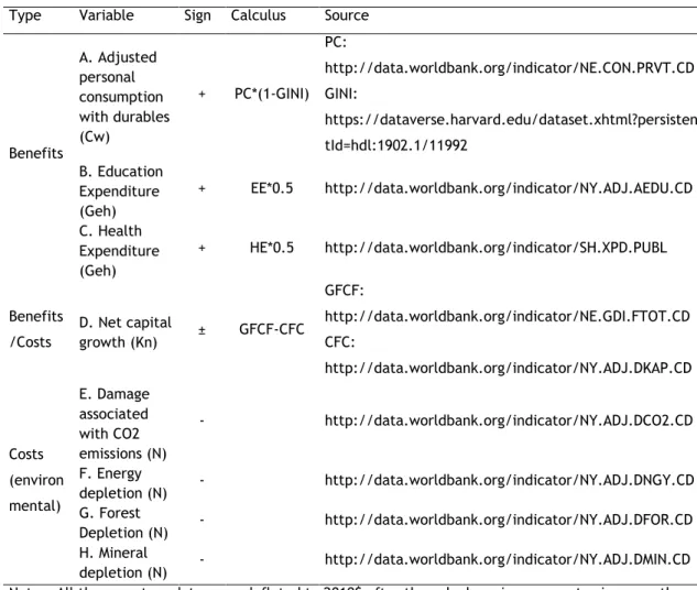
Table 1. ISEW type of components, variables, sign, calculus and data sources for all countries
Type Variable Sign Calculus Source
Benefits A. Adjusted personal consumption with durables (Cw) + PC*(1-GINI) PC: http://data.worldbank.org/indicator/NE.CON.PRVT.CD GINI: https://dataverse.harvard.edu/dataset.xhtml?persisten tId=hdl:1902.1/11992 B. Education Expenditure (Geh) + EE*0.5 http://data.worldbank.org/indicator/NY.ADJ.AEDU.CD C. Health Expenditure (Geh) + HE*0.5 http://data.worldbank.org/indicator/SH.XPD.PUBL Benefits /Costs D. Net capital growth (Kn) ± GFCF-CFC GFCF: http://data.worldbank.org/indicator/NE.GDI.FTOT.CD CFC: http://data.worldbank.org/indicator/NY.ADJ.DKAP.CD Costs (environ mental) E. Damage associated with CO2 emissions (N) - http://data.worldbank.org/indicator/NY.ADJ.DCO2.CD F. Energy depletion (N) - http://data.worldbank.org/indicator/NY.ADJ.DNGY.CD G. Forest Depletion (N) - http://data.worldbank.org/indicator/NY.ADJ.DFOR.CD H. Mineral depletion (N) - http://data.worldbank.org/indicator/NY.ADJ.DMIN.CD Notes: All the monetary data were deflated to 2010$ after the calculus, since current prices was the only available option in the WDI. The components following the definition are the ones used in Eq. (1). The Gini was applied as determinant of economic inequality (Gründler & Köllner, 2016). Only half of the expenditure in education and health is assumed to be defensive (Jackson et al. 1994).
11
It is worthwhile to make clear that in the computation of the ISEW, a few observations were calculated through growth averages due to the lack of data. For example, in the HIC, for Japan, information on the last two years was lacking for the ISEW indicator and so the growth rates for the past years were performed, summed all together and divided by the respective number of years, thus calculating the last two observations. In the UMIC, the same procedure was followed for Belarus, Kazakhstan, Malaysia and South Africa for the year 2013; and Iran and Thailand for the years 2012 and 2013. In the MLIC, the group with more information lacking, the countries Armenia, Egypt, Moldova and Philippines had the last year (2013) in fault. For India, Kyrgyz Republic, Nigeria, Pakistan, Vietnam, Senegal, Sierra Leone, Tanzania and Uganda the two last observations (2012 and 2013) were missing. Although, Rwanda, Sierra Leone and Uganda were not considered in the models but only in the descriptive analysis. Other countries with three or more gaps were immediately excluded from the sample.The methodology took into consideration in the study proceeds as follow: (1) the quality and nature of the data is observed; (ii) the issues of heteroscedasticity, serial correlation and contemporaneous correlation and cross-section dependence were assessed as well as the integration of the variables; (iii) since the study has the objective of analysing the short- and long-term interactions between food consumption, economic growth and sustainable development the ARDL approach is applied.
3.2. Descriptive Statistics
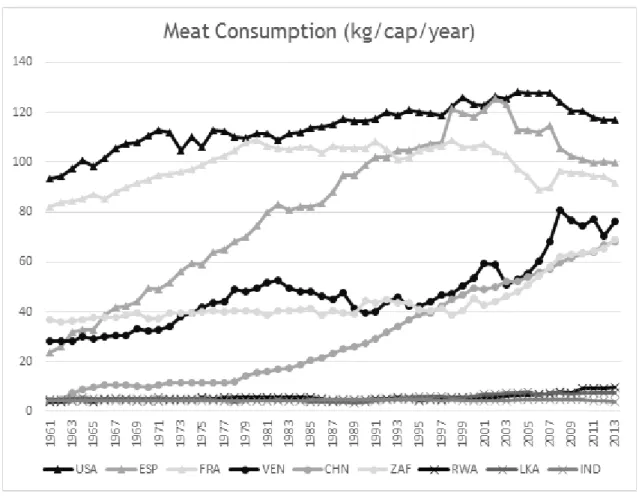
Following the established path, an initial analysis of the data is made. Putting the focus on meat consumption growth for the past 53 years, fig. 1 is provided. The figure corresponds to the three analysed groups of income and includes 3 countries of each. The triangle, circle and cross denote HIC, UMIC and MLIC, respectively. For the HIC the top three in terms of consumption in 2013 are displayed, for the UMIC, the three with the highest consumption rates for the whole period are analysed and for the MLIC, the bottom three least consuming countries are observed. Meat consumption is measured in kg/cap/year and the period goes from 1961 to 2013 for all countries.
From the figure, some global tendencies can be observed. First, a big difference of consumption between the three groups is evident. The HIC have an annual consumption of more than 100 kg per capita per year on average, where the UMIC do not even reach the 80 kg per capita per year. A much smaller consumption is clear in the MLIC analysed, consuming less than 10 kg per capita per year. The United States of America is the major consumer in the figure alongside Spain and France. India, having the smallest consumption, is a special case due to the fact that the majority of its citizens follows a vegetarian diet. Other aspect that can be deduced from the figure is the recent decreasing trend observed in all three HIC analysed, since the beginning of the century. Contrary to the brutal increasing trends from the UMIC. The country with the
12
highest increase is China, having more than quadrupled increased their consumption throughout the years. In Spain, it can be seen an increase from 24 kg per capita annually in 1961 to almost 100 kg per capita per year. As in Venezuela, from 28 to 76 kg per capita annually. While in China, a much dramatic increase is observed, from 4 kg per capita in 1961 to almost 70 kg per capita, an increase rate of more than 1500%. Although these dramatic increases exist in emerging economies, the poorer countries continue with lower levels of consumption throughout the years. Figures for the Sub-Saharan countries suggest broad differences in meat consumption between countries, with Nigeria, Rwanda, Sierra Leone and Tanzania on average below 10 kg per capita, around 15 kg per capita in Senegal and Uganda, in comparison with a meat consumption above 50 kg per capita, in recent years, in South Africa. Rwanda and the latter shown in the figure.
Fig. 1. Evolution of meat consumption in 3 countries of each income group, period 1961-2013
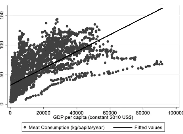
Furthermore, fig. 2 presents the relationship between meat consumption and income, for the overall sample. The main finding by observing the graph is that, in fact, income promotes meat consumption. We can see the massive dots in the left lower corner representing the poorer countries with small levels of meat consumption, in comparison with the more developed countries with higher levels of meat consumption. Therefore, by looking at the figure we can propose that, with higher levels of income, meat consumption increases, i.e., the relationship between income and meat consumption follows a positive linear framework. It can even be
13
suspected that a possible negative quadratic framework, similar to Kuznets, 1955, exists. Moreover, it can be deducted that at certain level of income, meat consumption starts to decrease. This is intensively explored by Vranken et al., 2014 where the authors empirically test this hypothesis concluding that in fact an inverted-U follows the relationship between meat consumption and income. Due to the need of consistency in the objective of this work, the hypothesis proposed will not be analysed.Fig. 2. Relationship between meat consumption and income per capita for all countries
Following our objective of studying the interactions between food, growth and development an additional figure is added to the analysis. Fig. 3 shows the relationship between income per capita and meat consumption. This perspective is new to the literature as discussed in sections above, but some findings can be directly highlighted through the figure below.
As it was observed in the following figure, at a first analysis it can be proposed a possible positive linear relationship between meat consumption and income, i.e., as meat consumption increases so does income, but at a lower rate, if compared to the inverse relationship. Although, the positive relationship can be observed, the graphic points out that there still exist many countries with reasonable levels of meat consumption but suffer from poor economic status. Others, on the other hand, with a relative increase in meat consumption see their economic level increase as well.
14
Fig. 3. Relationship between income per capita and meat consumption for all countries
To better understand the magnitude of meat consumption we can consider its average value for all countries, of nearly 60 kg per capita per year. By calculating the average meat consumption per day, we can understand the magnitude of the quantity consumed in our daily basis. Doing so, the average of meat consumption per day equals to 164 grams per capita.
According to McMichael et al., 2007, the authors suggest that in order to tackle the environmental degradation of the food industry a reduction to 90 grams per capita per day should be pursuit. Further explaining that to achieve such goal a reduction should be conducted in the developed world followed by an increase in meat consumption by the poorer countries. Comparing to the 90 grams per capita per day, the mean of the countries analysed is way much higher, almost the double. If we further compare by income level group we have a much higher meat consumption value of almost 85 kg per capita per year, giving a portion of 234 grams per capita of daily meat consumption in the HIC. More that the double compared to the goal proposed above. From this point, the mean values decrease, with a portion of 148 grams per capita of daily meat consumption in the UMIC and 60 grams per capita per day from the MLIC. From these only 27 grams per capita are consumed daily in the five LIC analysed. Overall, the disparity in consumption is very large. Considering the 90 grams per capita per day goal a reduction of more than half of meat consumption needs to be pursued in the developed world and a more than reasonable increase in the poorer regions.
15
3.3. Methods
Since the focus of this study is to analyse the interactions between food consumption, economic growth and sustainable development, and considering the recent concern with dietary habits and as a reference for future generations, it was decided to pursuit an analysis of the dynamic effects in the short- and long-run. The Autoregressive Distributed Lag (ARDL) has the characteristic of analysing both effects separately (Pesaran & Shin, 1999). Another advantage is its robustness in front of different integration order of the variables, i.e., I(0), I(1) or both, but not I(2). Considering two approaches, namely the economic approach and the sustainable approach, applying the GDP and the ISEW, respectively; and further analysing between different income groups, specifically HIC, UMIC and MLIC, twelve models were estimated. Table A.2. is provided with the models notations to further facilitate the analysis. The general specification of the ARDL models for a specific income level are as follows:
𝐿𝑀𝐶𝑃𝐶 = ʄ (𝐿𝐺𝐷𝑃𝑃𝐶; 𝐿𝑃𝐵𝐶𝑃𝐶; 𝐿𝐹𝑆𝑃; 𝐿𝑋𝑁𝐼; 𝐿𝐾𝑂𝐹; 𝐿𝐿; 𝐿𝐶𝑃𝐼) (2) 𝐿𝑀𝐶𝑃𝐶 = ʄ (𝐿𝐼𝑆𝐸𝑊𝑃𝐶; 𝐿𝑃𝐵𝐶𝑃𝐶; 𝐿𝐹𝑆𝑃; 𝐿𝑋𝑁𝐼; 𝐿𝐾𝑂𝐹; 𝐿𝐿; 𝐿𝐶𝑃𝐼) (3) 𝐿𝐺𝐷𝑃𝑃𝐶 = ʄ (𝐿𝑀𝐶𝑃𝐶; 𝐿𝑃𝐵𝐶𝑃𝐶; 𝐿𝐹𝑆𝑃; 𝐿𝑋𝑁𝐼; 𝐿𝐸𝑈𝑃𝐶; 𝐿𝐾𝑂𝐹; 𝐿𝐺𝐹𝐶𝐹𝑃𝐶; 𝐿𝐿; 𝐿𝐶𝑃𝐼) (4) 𝐿𝐼𝑆𝐸𝑊𝑃𝐶 = ʄ (𝐿𝑀𝐶𝑃𝐶; 𝐿𝑃𝐵𝐶𝑃𝐶; 𝐿𝐹𝑆𝑃; 𝐿𝑋𝑁𝐼; 𝐿𝐸𝑈𝑃𝐶; 𝐿𝐾𝑂𝐹; 𝐿𝐺𝐹𝐶𝐹𝑃𝐶; 𝐿𝐿; 𝐿𝐶𝑃𝐼) (5)
The empirical models, where the short- and long-run dynamics are presented, i.e., the ARDL equivalent of the general unrestricted error correction model (UECM), for the four panels are specified as follows: ∆𝐿𝑀𝐶𝑃𝐶𝑖𝑡= 𝛼𝑖+ ∑ 𝛽1𝑖𝑗∆𝐿𝐺𝐷𝑃𝑃𝐶𝑖𝑡 𝑛 𝑗=0 + ∑ 𝛽2𝑖𝑗∆𝐿𝑃𝐵𝐶𝑃𝐶𝑖𝑡 𝑛 𝑗=0 + ∑ 𝛽3𝑖𝑗∆𝐿𝐹𝑆𝑃𝑖𝑡 𝑛 𝑗=0 + ∑ 𝛽4𝑖𝑗∆𝐿𝑋𝑁𝐼𝑖𝑡 𝑛 𝑗=0 + ∑ 𝛽5𝑖𝑗∆𝐿𝐾𝑂𝐹𝑖𝑡 𝑛 𝑗=0 + ∑ 𝛽6𝑖𝑗∆𝐿𝐿𝑖𝑡 𝑛 𝑗=0 + ∑ 𝛽7𝑖𝑗∆𝐿𝐶𝑃𝐼𝑖𝑡 𝑛 𝑗=0 + 𝛿1𝑖𝐿𝑀𝐶𝑃𝐶𝑖𝑡−1 + 𝛿2𝑖𝐿𝐺𝐷𝑃𝑃𝐶𝑖𝑡−1+ 𝛿3𝑖𝐿𝑃𝐵𝐶𝑃𝐶𝑖𝑡−1+ 𝛿4𝑖𝐿𝐹𝑆𝑃𝑖𝑡−1+ 𝛿5𝑖𝐿𝑋𝑁𝐼𝑖𝑡−1+ 𝛿6𝑖𝐿𝐾𝑂𝐹𝑖𝑡−1 + 𝛿7𝑖𝐿𝐿𝑖𝑡−1+ 𝛿8𝑖𝐿𝐶𝑃𝐼𝑖𝑡−1+ 𝜀𝑖𝑡 (6) ∆𝐿𝑀𝐶𝑃𝐶𝑖𝑡= 𝛼𝑖+ ∑ 𝛽1𝑖𝑗∆𝐿𝐼𝑆𝐸𝑊𝑃𝐶𝑖𝑡 𝑛 𝑗=0 + ∑ 𝛽2𝑖𝑗∆𝐿𝑃𝐵𝐶𝑃𝐶𝑖𝑡 𝑛 𝑗=0 + ∑ 𝛽3𝑖𝑗∆𝐿𝐹𝑆𝑃𝑖𝑡 𝑛 𝑗=0 + ∑ 𝛽4𝑖𝑗∆𝐿𝑋𝑁𝐼𝑖𝑡 𝑛 𝑗=0 + ∑ 𝛽5𝑖𝑗∆𝐿𝐾𝑂𝐹𝑖𝑡 𝑛 𝑗=0 + ∑ 𝛽6𝑖𝑗∆𝐿𝐿𝑖𝑡 𝑛 𝑗=0 + ∑ 𝛽7𝑖𝑗∆𝐿𝐶𝑃𝐼𝑖𝑡 𝑛 𝑗=0 + 𝛿1𝑖𝐿𝑀𝐶𝑃𝐶𝑖𝑡−1 + 𝛿2𝑖𝐿𝐼𝑆𝐸𝑊𝑃𝐶𝑖𝑡−1+ 𝛿3𝑖𝐿𝑃𝐵𝐶𝑃𝐶𝑖𝑡−1+ 𝛿4𝑖𝐿𝐹𝑆𝑃𝑖𝑡−1+ 𝛿5𝑖𝐿𝑋𝑁𝐼𝑖𝑡−1+ 𝛿6𝑖𝐿𝐾𝑂𝐹𝑖𝑡−1 + 𝛿7𝑖𝐿𝐿𝑖𝑡−1+ 𝛿8𝑖𝐿𝐶𝑃𝐼𝑖𝑡−1+ 𝜀𝑖𝑡 (7)
16
∆𝐿𝐺𝐷𝑃𝑃𝐶𝑖𝑡= 𝛼𝑖+ ∑ 𝛽1𝑖𝑗∆𝐿𝑀𝐶𝑃𝐶𝑖𝑡 𝑛 𝑗=0 + ∑ 𝛽2𝑖𝑗∆𝐿𝑃𝐵𝐶𝑃𝐶𝑖𝑡 𝑛 𝑗=0 + ∑ 𝛽3𝑖𝑗∆𝐿𝐹𝑆𝑃𝑖𝑡 𝑛 𝑗=0 + ∑ 𝛽4𝑖𝑗∆𝐿𝑋𝑁𝐼𝑖𝑡 𝑛 𝑗=0 + ∑ 𝛽5𝑖𝑗∆𝐿𝐾𝑂𝐹𝑖𝑡 𝑛 𝑗=0 + ∑ 𝛽6𝑖𝑗∆𝐿𝐸𝑈𝑃𝐶𝑖𝑡 𝑛 𝑗=0 + ∑ 𝛽7𝑖𝑗∆𝐿𝐺𝐹𝐶𝐹𝑃𝐶𝑖𝑡 𝑛 𝑗=0 + ∑ 𝛽8𝑖𝑗∆𝐿𝐿𝑖𝑡 𝑛 𝑗=0 + ∑ 𝛽9𝑖𝑗∆𝐿𝐶𝑃𝐼𝑖𝑡 𝑛 𝑗=0 + 𝛿1𝑖𝐿𝐺𝐷𝑃𝑃𝐶𝑖𝑡−1+ 𝛿2𝑖𝐿𝑀𝐶𝑃𝐶𝑖𝑡−1+ 𝛿3𝑖𝐿𝑃𝐵𝐶𝑃𝐶𝑖𝑡−1 + 𝛿4𝑖𝐿𝐹𝑆𝑃𝑖𝑡−1+ 𝛿5𝑖𝐿𝑋𝑁𝐼𝑖𝑡−1+ 𝛿6𝑖𝐿𝐾𝑂𝐹𝑖𝑡−1+ 𝛿7𝑖𝐿𝐸𝑈𝑃𝐶𝑖𝑡−1+ 𝛿8𝑖𝐿𝐺𝐹𝐶𝐹𝑃𝐶𝑖𝑡−1 + 𝛿9𝑖𝐿𝐿𝑖𝑡−1+ 𝛿10𝑖𝐿𝐶𝑃𝐼𝑖𝑡−1+ 𝜀𝑖𝑡 (8) ∆𝐿𝐼𝑆𝐸𝑊𝑃𝐶𝑖𝑡= 𝛼𝑖+ ∑ 𝛽1𝑖𝑗∆𝐿𝑀𝐶𝑃𝐶𝑖𝑡 𝑛 𝑗=0 + ∑ 𝛽2𝑖𝑗∆𝐿𝑃𝐵𝐶𝑃𝐶𝑖𝑡 𝑛 𝑗=0 + ∑ 𝛽3𝑖𝑗∆𝐿𝐹𝑆𝑃𝑖𝑡 𝑛 𝑗=0 + ∑ 𝛽4𝑖𝑗∆𝐿𝑋𝑁𝐼𝑖𝑡 𝑛 𝑗=0 + ∑ 𝛽5𝑖𝑗∆𝐿𝐾𝑂𝐹𝑖𝑡 𝑛 𝑗=0 + ∑ 𝛽6𝑖𝑗∆𝐿𝐸𝑈𝑃𝐶𝑖𝑡 𝑛 𝑗=0 + ∑ 𝛽7𝑖𝑗∆𝐿𝐺𝐹𝐶𝐹𝑃𝐶𝑖𝑡 𝑛 𝑗=0 + ∑ 𝛽8𝑖𝑗∆𝐿𝐿𝑖𝑡 𝑛 𝑗=0 + ∑ 𝛽9𝑖𝑗∆𝐿𝐶𝑃𝐼𝑖𝑡 𝑛 𝑗=0 + 𝛿1𝑖𝐿𝐼𝑆𝐸𝑊𝑃𝐶𝑖𝑡−1+ 𝛿2𝑖𝐿𝑀𝐶𝑃𝐶𝑖𝑡−1+ 𝛿3𝑖𝐿𝑃𝐵𝐶𝑃𝐶𝑖𝑡−1 + 𝛿4𝑖𝐿𝐹𝑆𝑃𝑖𝑡−1+ 𝛿5𝑖𝐿𝑋𝑁𝐼𝑖𝑡−1+ 𝛿6𝑖𝐿𝐾𝑂𝐹𝑖𝑡−1+ 𝛿7𝑖𝐿𝐸𝑈𝑃𝐶𝑖𝑡−1+ 𝛿8𝑖𝐿𝐺𝐹𝐶𝐹𝑃𝐶𝑖𝑡−1 + 𝛿9𝑖𝐿𝐿𝑖𝑡−1+ 𝛿10𝑖𝐿𝐶𝑃𝐼𝑖𝑡−1+ 𝜀𝑖𝑡 (9)The prefixes “Δ” and “L” denote first differences and natural logarithms of the variables, respectively. The subscripts i, j and t denote country, lag length and time period, respectively. The intercept is denoted as α, βi and δi are the estimated parameters, and εit the error term.
The natural logarithms were applied to facilitate the interpretation of the elasticities and semi-elasticities, as they are presented as percentages and percentage points (pp), respectively.
In order to proceed with this panel data approach some characteristics are required in respect of the data. The presence of cross-sectional dependence is analysed by using the CD-test. Results revealed in tables A.3. – A.5. show that cross-sectional dependence is present, which could be explained by the income level proximity of the countries analysed within each income group. Considering the presence of cross-sectional dependence, determining whether the data is stationary or integrated is essential. To do so, second generation unit root tests CIPS (M. Hashem Pesaran, 2007) were applied. The results for each of the income groups are displayed in table A.6., in the appendix. By looking at the results we can observe that not all the variables are stationary in levels. Although, by applying the differences, we can conclude that all variables are stationary in first differences, thus confirming that the variables are all integrated of first order, i.e., I(1). As such, these outcomes confirm the appropriateness of the use of the ARDL approach. Additionally, multicollinearity between the variables was also tested using the variance inflation factor (VIF). The results show that the VIF values are all less than 5, suggesting that this issue will not be a problem.
17
In terms of the choice for the most efficient estimator, the Robust Hausman test (sigmamore option suggested by Cameron & Trivedi, 2010) to select between the fixed effects (FE) and random effects (RE) estimators was applied. The null hypothesis is that random effects is suitable instead of fixed effects. The null hypothesis is rejected in all the models following the results shown in tables 2-3, with at least 5% significance. Therefore, considering that the FE estimator is the most suitable for the present study. The possibility of a heterogeneous panel is not considered, mainly due to the fact that countries were grouped according to their income level. By doing so, the risk of being faced with a heterogeneous panel is severely reduced, as it can be considered that the cross sections share common coefficients.From this point, additional specifications are required with the purpose to understand the robustness of the estimator. The presence of heteroscedasticity, autocorrelation and contemporaneous correlation among cross sections was analysed. The results of all tests are reported in tables 2-3.
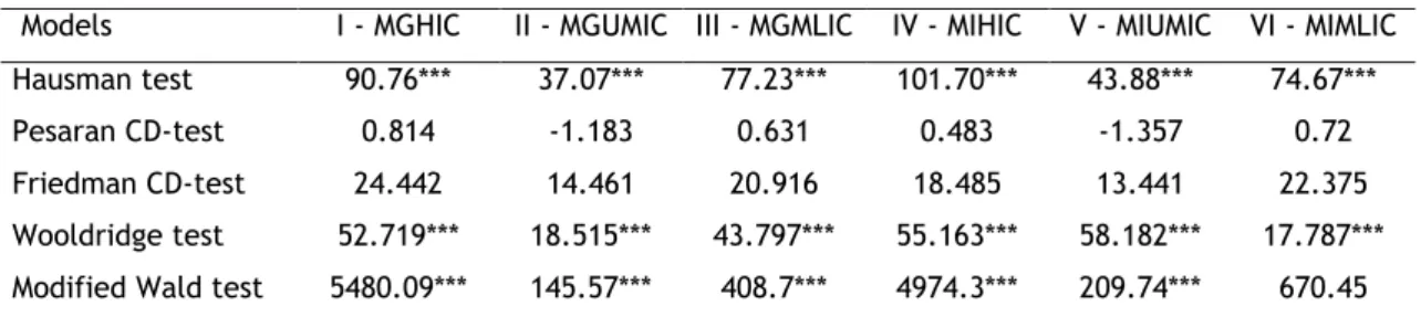
Table 2. Specification tests
Models I - MGHIC II - MGUMIC III - MGMLIC IV - MIHIC V - MIUMIC VI - MIMLIC Hausman test 90.76*** 37.07*** 77.23*** 101.70*** 43.88*** 74.67*** Pesaran CD-test 0.814 -1.183 0.631 0.483 -1.357 0.72 Friedman CD-test 24.442 14.461 20.916 18.485 13.441 22.375 Wooldridge test 52.719*** 18.515*** 43.797*** 55.163*** 58.182*** 17.787*** Modified Wald test 5480.09*** 145.57*** 408.7*** 4974.3*** 209.74*** 670.45 Notes: The Hausman test has a
χ
2 and tests H0 that unobservable individual effects are not correlated with the explanatory variables; Pesaran and Friedman’s test are parametric testing procedures and follow a standard normal distribution; The Wooldridge test is normally distributed N(0,1) and tests H0 no serial correlation; The Modified Wald test has
χ
2 distribution and tests H0 no heteroscedasticity; Significance notation for 1, 5 and 10% are denoted as ***, **, *, respectively.
Table 3. Specification tests (cont.)
Models VII - GMHIC VIII - GMUMIC IX - GMMLIC X - IMHIC XI - IMUMIC XII - IMMLIC Hausman test 57.5*** 50.98*** 48.61*** 96.5*** 82.86*** 51.99*** Pesaran CD-test 20.657*** 21.654*** 26.268*** 40.626*** 39.223*** 42.183*** Friedman CD-test 125.171*** 125.707*** 156.44*** 243.907*** 225.29*** 243.296*** Wooldridge test 60.032*** 80.64*** 157.528*** 108.044*** 137.553*** 143.606*** Modified Wald test 925.2*** 1023.59*** 6931.09*** 4910.03*** 1086.08*** 3153.66*** Notes: The Hausman test has a
χ
2 and tests H0 that unobservable individual effects are not correlated with the explanatory variables; Pesaran and Friedman’s test are parametric testing procedures and follow a standard normal distribution; The Wooldridge test is normally distributed N(0,1) and tests H0 no serial correlation; The Modified Wald test has
χ
2 distribution and tests H0 no heteroscedasticity; Significance notation for 1, 5 and 10% are denoted as ***, **, *, respectively.
The phenomenon of group-wise heteroscedasticity was checked using the modified Wald test, developed by Greene, 2012. The null hypothesis of no heteroscedasticity present in the errors was rejected in all the models, suggesting that heteroscedasticity is present. Furthermore, the Wooldridge test (Wooldridge, 2010) detected the presence of autocorrelation in all the models
18
as well, by rejecting the null hypothesis of no autocorrelation in the errors, with high significance, at the 1% level. For the appraisal of contemporaneous correlation among cross sections, two tests were conducted, the Pesaran test and the Friedman test. Both tests point out that not all the models suffer from the existence of contemporaneous correlation. Considering the results of the specification tests, two estimators were chosen for the regressions. The Driscoll and Kraay estimator (Driscoll & Kraay, 1998) was applied in the models where contemporaneous correlation was present, since the standard errors of the latter are robust in these conditions, alongside heteroscedasticity and autocorrelation. The FE model with robust standard errors was estimated in the models where contemporaneous correlation was not existent, considering only heteroscedasticity and autocorrelation. The results are analysed in the next section.
4. Empirical Results
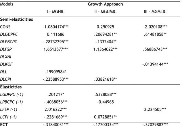
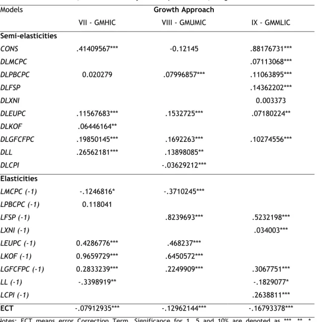
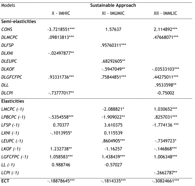
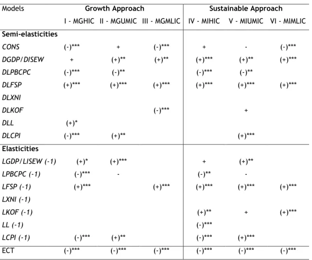
The ARDL approach with the Driscoll-Kraay (DK) and the FE Robust with clusters are estimated for all the three income groups and respective analysis generating a total of twelve models. Once again, the analysis of this study is tripartite. The procedure involves (1) an analysis between income level groups is made under the same model, i.e., applying the same dependent variable, (2) a comparison is made within the same income level groups, i.e., an assessment between the conventional growth indicator, GDP, and the sustainable development ISEW and (3) an analysis is made around the interactions already mentioned by analysing both variables as explaining meat consumption and as explained by meat consumption. To preserve space, the reduced estimation results are presented in tables A.7. – A.10. in the Appendix. The elasticities and semi-elasticities are revealed on the next subsection.
Before analysing the impact of the parameters, the consistency of the models is observed. To evaluate whether the estimations are able to explain part of the variations in the dependent variables analysed, namely meat consumption, economic growth and sustainable development, the F-tests were performed for each estimation, testing for the joint significance of all the included variables. As it can be observed in tables A.7 – A.10. in the appendix, for all the models, the F-tests reject the null hypothesis, with the highest significance (1%), that there is no joint effect of the included explanatory variables. Thus, concluding that the included variables have some explanatory power for the changes in eat consumption, economic growth and sustainable development. Regarding the error correction term (ECT), which reveals the speed adjustment of the model given a specific shock. Considering an impact in the short-run, the ECT indicates how long is needed for the model to readjust. For example, in model (I - MGHIC) the ECT is of -0.3184, indicating that the time the models needs to adjust is a bit less than 3 years. Contrary to model (VII - GMHIC), which needs more than 10 years to adjust (-0.07913). To assess the magnitude of the effects, both semi-elasticities and elasticities were performed (tables 4-7).
19
4.1. Does income promote meat consumption?
From tables 4-5, the results of the analysis of meat consumption through the economic growth approach show that major statistically significances for food consumption, at least in the short- or long-run, for all countries. In table 4 the effects of economic growth on meat consumption are as expected. All income level groups showing a positive impact. The higher effect is observed in the poorer countries, although only in the short-run. The semi-elasticities can be read as, with a 1 percentage point (pp) increase in a certain variable, the dependent increases in the order of the elasticity of semi-elasticity value in pp terms. Therefore, a 1 pp increase in the GDP per capita follows a 0.614 pp increase in meat consumption in the MLIC, analysing the short-term. By doing the same analysis in the HIC and UMIC we have an 0.112 and 0.207 pp increase in meat consumption, respectively. Although with no statistically significance for the HIC, but at the 5% level for the UMIC. Larger impacts are observed in the long-run for both HIC and UMIC. The analysis of the elasticities is different, as a 1% increase in the parameter analysed contributes to an increase in percentage, of the value observed in the elasticity. Thus, the impacts are of 0.201% in HIC and 0.533% in UMIC. In terms of plant-based consumption, the expected is confirmed as well. In the developed countries, a negative effect is observed both in the short- as in the long-run. In the HIC an increase of 1 pp and 1% in plant-based consumption follows an impact of -0.287 pp and -0.407% in the short- and long-run, respectively. As it is seen in the UMIC, impacts of -0.133 pp and -0.45%, as in the above order. Although the latter not statistically significant.
Table 4. Semi-elasticities, elasticities and adjustment speed for MC with GDP, using FE Cluster
Models Growth Approach
I - MGHIC II - MGUMIC III - MGMLIC
Semi-elasticities CONS -1.0804174*** 0.290925 -2.020108*** DLGDPPC 0.111686 .20694281** .61481858** DLPBCPC -.28732295*** -.1332404** DLFSP 1.6512577*** 1.1364022*** .56886743*** DLXNI DLKOF -.01394144*** DLL .19909584* DLCPI -.23588953*** .03821618** Elasticities LGDPPC (-1) .201217* .5328088*** LPBCPC (-1) -.4068056*** -0.44965 LFSP (-1) 2.016222*** 2.224505*** LCPI (-1) -.2281669*** 0.0728851** ECT -.31840031*** -.17700334*** -.32029882***
Notes: ECT means Error Correction Term. Significance notation for 1, 5 and 10% are denoted as ***, **, *, respectively.