Paulo Jorge Baptista Vieira
MESTRADO EM ECONOMIA
Fevereiro | 2011
An Essay on Economic Growth - Classical
Determinants, Convergence and Financial Development
Paulo Jorge Baptista Vieira
DM
An Essay on Economic Growth - Classical
Determinants, Convergence and Financial Development
DISSERTAÇÃO DE MESTRADO
DIMENSÕES: 45 X 29,7 cm
Tese de Mestrado em Economia
“An Essay on Economic Growth: Classical Determinants, Convergence and Financial Development”
Aluno Orientador
Paulo Jorge Baptista Vieira Prof. Doutor Corrado Andini
Nº 2002008 Universidade da Madeira
February 2011
ACKNOWLEDGEMENTS
I would like to thank Prof. Dr. Corrado Andini for his guidance and helpful suggestions. I also benefited of the comments from my colleague Renato Marques and the advice of Dionísio Nascimento. A special thanks to Antonio Correia for helping me to access the b-on database.
The usual disclaimer applies.
CONTENTS
1.INTRODUCTION...5
2. THE SOLOW MODEL AND ITS PREDECESSORS...7
2.1THE SOLOW MODEL ...8
2.2 A BRIEF NOTE ON ENDOGENOUS GROWTH THEORIES... 13
3. EMPIRICAL STUDIES ON ECONOMIC GROWTH ...15
3.1MAIN PROBLEMS IN GROWTH REGRESSIONS...16
3.2THE IMPORTANCE OF HUMAN CAPITAL...19
3.2.1 LEAMER’S SENSITIVITY ANALYSIS...26
3.3RUNNING MILLIONS OF REGRESSIONS ...31
4.WHAT ABOUT CONVERGENCE?...36
4.1CONDITIONAL CONVERGENCE AND σ AND β CONVERGENCE...36
4.1.1.EMPIRICAL STUDIES ON THE SUBJECT OF CONVERGENCE ....37
4.1.1.1 CONVERGENCE AND CROSS-SECTION REGRESSIONS...37
4.1.1.2 EVALUATING CONVERGENCE USING PANEL DATA ...41
4.1.1.3 EVALUATING CONVERGENCE USING QUANTILE REGRESSIONS..46
5.FINANCE AND GROWTH...53
5.1IS SCHUMPETER RIGHT?...54
5.2. STOCK MARKET AND GROWTH... 73
6.CONCLUSIONS...81
ABSTRACT
This dissertation surveys the literature on economic growth. I review a substantial number of articles published by some of the most renowned researchers engaged in the study of economic growth. The literature is so vast that before undertaking new studies it is very important to know what has been done in the field. The dissertation has six chapters. In Chapter 1, I introduce the reader to the topic of economic growth. In Chapter 2, I present the Solow model and other contributions to the exogenous growth theory proposed in the literature. I also briefly discuss the endogenous approach to growth. In Chapter 3, I summarize the variety of econometric problems that affect the cross-country regressions. The factors that contribute to economic growth are highlighted and the validity of the empirical results is discussed. In Chapter 4, the existence of convergence, whether conditional or not, is analyzed. The literature using both cross-sectional and panel data is reviewed. An analysis on the topic of convergence using a quantile-regression framework is also provided. In Chapter 5, the controversial relationship between financial development and economic growth is analyzed. Particularly, I discuss the arguments in favour and against the Schumpeterian view that considers financial development as an important determinant of innovation and economic growth. Chapter 6 concludes the dissertation. Summing up, the literature appears to be not fully conclusive about the main determinants of economic growth, the existence of convergence and the impact of finance on growth.
RESUMO
Esta dissertação versa sobre a literatura relacionada com temas de crescimento económico. É feita a análise de um número significativo de artigos publicados por alguns dos mais reconhecidos investigadores que se dedicam ao estudo do crescimento económico. A literatura é tão vasta que antes de se empreender novo estudo empírico é muito importante saber o que está feito na área. Esta dissertação é composta de seis capítulos. O capítulo 1 é uma introdução ao tema do crescimento económico. No capítulo 2, apresenta-se o modelo de Solow e outras contribuições à teoria de crescimento exógeno propostas na literatura. De forma resumida, é feita também referência às teorias de crescimento endógeno. O capítulo 3 contém uma síntese da variedade de problemas econométricos que afectam principalmente as regressões com dados seccionados por país. De seguida, são expostos os factores que contribuem para o crescimento económico bem como a discussão à volta da validade desses resultados. No capítulo 4, a existência de convergência, seja ela condicional ou não, é também abordada, começando-se por rever a literatura que assenta em regressões com dados seccionados e com dados de painel. É feita ainda uma análise à questão da convergência à luz de métodos assentes em regressões quantílicas. No capítulo 5, a controversa relação entre o desenvolvimento financeiro e crescimento é também abordada. São discutidos os argumentos a favor e contra a visão schumpeteriana, que considera que os instrumentos financeiros são importantes para a inovação e crescimento económico. O capítulo 6 conclui a dissertação, sendo que muitas das questões relacionadas com os determinantes do crescimento económico, a existência da convergência e o impacto do desenvolvimento financeiro no crescimento, não encontram respostas unívocas na literatura.
Palavras-chave: Crescimento Económico; Convergência; Desenvolvimento
1. INTRODUCTION
One of the eternal discussions in economic science is about the nature and characteristics of economic growth. This debate started long time ago, with economists trying to decipher the factors that drive or hinder growth, whether there is convergence among countries and if so at what speed.
The model created by Robert Solow, published in 1956, is the starting point of the investigation made in the last 54 years. Many of the most relevant articles that have been published since then, tried to test, criticize or expand it. The development of computers and appropriate software in the 1980’s made possible to test empirically the Solow model, with its variants and alternatives.
In this dissertation I chose to focus on three topics: the discussion about the factors that determine growth, the debate about convergence and the relationship between finance (including the stock market) and growth. A selection of the relevant articles on these topics was made, as I try to summarize and interconnect them when possible. The literature on this subject is too vast. Some works are only briefly discussed and others are inevitably left out, which does not mean that they are not relevant.
As usual in the field of scientific investigation, it is difficult to draw absolute truths, so the debate will go on…
Understanding the process of economic growth is an important starting point to build up more effective development strategies. It is fundamental to examine this process in all its complexity, considering the economic, social and political dimensions. In doing so, a lot of questions arise:
- Who are the winners and the losers in the growth process?
- Why does the population of the countries with higher growth rates do not necessarily have a correspondent human development level?
- What form of government and governance is more suited to economic
growth and development?
- What is the most efficient combination of economic actors/players?
2. THE SOLOW MODEL AND ITS PREDECESSORS
Historically, there are four models that form the basis of modern thought on economic growth. The first is the model of Adam Smith (1776). However to consider it a model is somehow far-fetched. Smith established a link between the process of specialization (resulting from international trade or from a market
size increase) and the total output of an economy, i.e., more specialization
brings an increase in an economy’s output.
The model of Malthus (1798, 1803) is the first to relate, in a comprehensive and systematic way, growth with changes in the population. Taking the concept of diminishing returns, Malthus foresaw stagnation in the long run, the result of steady population growth, which annulled the increases in
real output per capita.
We can attribute the third model to Joseph Schumpeter (1912), who exacerbates the role of innovation and creative destruction, which is nothing more than replacing old processes with new, something that can lead the economy to a higher degree.
saving. The weakest point of the model was in the constancy of the capital-output ratio.
Obviously I could mention other models, such as that presented by David Ricardo, who considered international trade and comparative advantages, as ways that allow the economies to overcome stagnation.
Karl Marx had more radical ideas. Cutting with classical thinking, he advocated the weakening of capital and strengthening of labour due to a declining rate of profit that would result from imbalances in the capitalist system. This would generate overproduction on one hand and in the other hand a failure in the ability to redistribute income (damaging the working classes).
Going back to the twentieth century, I will now focus in the Solow model. This model suggests that technology is the cause of long-term economic growth. It does not establish a linear relationship between savings and growth, and considers that the saving rate and investment have not a long-term effect on economic growth. The simplicity of the model, combined with the ability to distinguish the sources of growth in the short, medium and long term contributed to labelling it as a reference model after more than 50 years since its publication.
2.1 THE SOLOW MODEL
Solow (1956) makes an analysis inspired by neoclassical authors of the nineteenth century, and that is why the model is known as the neoclassical growth model.
Let us now look more carefully to the basic structure of Solow’s model.
We start with the production function given by:
) (k f
y , with L K
k (1)
Therefore economic growth is defined in terms of output per capita. Each
increase in K relatively to L will cause smaller and smaller increments of y.
The Consumption per worker function is defined by:
y s p
y
c (1 ) (2)
where s is the rate of saving and p stands for savings per employee.
The stock of capital increases with investment (savings), but is affected by the phenomenon of depreciation. In per worker terms we have:
k k
f s k y s k i
k
( ) (3)
where i is investment per capita and the depreciation rate.
In order for K to be constant, the investment, i, must be great enough to
cover for the capital that depreciates and the equipment of new workforce units. Adding this feature, we have:
k n k
f k
n k i
k
( ) ( ) (4)
where n is the rate of increase in labour force.
Countries with higher population growth rates have lower levels of output
per capita. Thus, the obvious candidate to explain growth in the Solow model
turns out to be technological progress, which can be described as a better ability of a country in converting resources into welfare by increasing production. Economic and cultural factors can matter too (trade union restrictions, environmental restrictions, etc…).
This part of output growth which cannot be attributed to the accumulation of capital and labour is called the Solow residual. It is related to efficiency in the use of these factors, and the measure of this efficiency is usually referred to as Total Factor Productivity.
Technological progress improves the efficiency of the labour force. So, our production function can be now defined by:
)] ( [K L E F
Y (5)
E, being the efficiency of each worker.
The variation of the capital stock per efficient unit is:
k g n
k f s k g n
i
kˆ ( ) ˆ (ˆ)( ) ˆ
where g stands for the rate of improvement of the work efficiency through
technological progress, and
E L
K k
ˆ .
Therefore, the higher the savings rate, the higher the output per worker. The Solow model predicts that the economy will evolve into a steady state, a point where there is no growth in output (or in capital stock). Keep in mind that
s, n, g and are exogenous.
The economy tends toward a steady state (see figure 1, below) when
△ k = 0, i.e.:
*
*) ( )
(k n g k
f
s (7)
In steady state, income per efficiency unit is constant (yˆ*=f(kˆ*)), while
income per person grows at rate g, and total income grows at rate (n+g).
Figure 1. Steady state with technological progress
In figure 2 below (y and k are in per capita terms), we can see the effect of
technological progress in the production function. The initial steady state for
income per capita is y1. With technology progress, the production function shifts
f(k)
(δ+n+g).
kˆ
from f1(k) to f2(k). This will have a repercussion in the total savings (σ.f1(k)),
and so k will also rise, changing income per capita from y1to y2.
Figure 2. Technological progress and economic growth
Mankiw (1995) lists the predictions of the Solow model:
1. In the long run, the economy approaches a steady state which is
independent of initial conditions;
2. A higher saving rate leads to a higher steady state level of income per
person, while a higher rate of population growth has the opposite effect;
3. It is the technological progress that influences the steady state rate of
growth of income per person;
4. In the steady state, the capital-to-income ratio is constant;
5. In the steady state, the marginal product of capital is constant, and the
marginal product of labour grows at the rate of technological progress.
These predictions have been evaluated over time, especially 2, 4 and 5.
criticisms concerning this neoclassical growth model. Neither the fact that technological progress is exogenous (which motivated the appearance of the theories of endogenous growth), nor the apparent unrealistic option of considering the same production function for all countries are strong enough to discard Solow’s model.
Durlauf, Kourtellos and Minkin (2001) do not share the same opinion. They state that there is a substantial country-specific heterogeneity in Solow’s model parameters, which is associated with differences in initial income. To prove this, they built a model which incorporates this heterogeneity and the results show that the explanatory value of the Solow model increases strongly
when using differentiated production functions. Durlauf et al. conclude that
empirical exercises that neglect this factor lead to misleading results.
However, Mankiw (1995) points out three main problems about the validity of the Solow model. First, the model does not reflect the disparity in international living standards (the absence of human capital as a variable could explain this). In second place, the rate of convergence that the model predicts is twice the rate that actually occurs, which is about 2 percent per year according to most studies. The third problem is in the fact that the return to capital differentials between countries predicted by the Solow model is much greater than that observed empirically.
2.2 A BRIEF NOTE ON ENDOGENOUS GROWTH THEORIES
To avoid the assumption of exogenous advances in technology, some researchers have developed endogenous growth theories. One of the best known is the AK model, created by Rebelo (1991).
k Y s
K
(8)
implying that:
A s K
K Y
Y
(9)
As long as s.A is greater than δ, income will grow indefinitely, even without
assuming an exogenous technological progress. In this case, saving will lead to permanent growth, in opposition to the neoclassical model. The AK model is the simplest of all endogenous growth models. However the AK is unable to explain growth in the last 200 years, since investment in physical capital cannot,
alone by itself, explain the rising of the world GDP per capita.
3. EMPIRICAL STUDIES ON ECONOMIC GROWTH
The Solow model dates from the 1950´s, however empirical tests have become common more recently, with the most prominent works being published in the last 25 years. The important work of Summers and Heston (1991) was fundamental to make international data suitable for cross-section analysis for the majority of the world countries.
In the typical empirical papers on economic growth, the authors gather a sample of countries and then run a cross-sectional regression. Usually, on one side we have the countries average growth rate and on the other side a set of variables that may or may not determine that growth rate. Of course the variables change from study to study, and also the interpretation of the results.
Mankiw (1995) points out the most important findings:
- the existence of conditional convergence, i.e. a low initial level of
income is associated with a high subsequent growth rate when other variables are held constant;
- the share of output allocated to investment is positively related to growth
as well as enrolment rates in primary and secondary schools (both measures of human capital);
- population growth is negatively related with growth in income per
capita, as well as political instability and market distortions (impediments to trade, black market premium to foreign exchange);
- countries with better developed financial markets, tend to have higher
3.1 MAIN PROBLEMS IN GROWTH REGRESSIONS
However there is a lot of discussion about the validity of some results, and most of the time, the root of this discussion is in some problems that affect growth regressions.
According to Mankiw (1995), three different types of problems arise in cross-country growth regressions: simultaneity, multicollinearity and the degrees of freedom problem.
Simultaneity happens when the right-hand-side variables are not in fact, exogenous.
Let us focus on investment and growth. Which causes which? Or is there a third variable that causes both investment and growth? The solution is to find exogenous variables to use as instruments, which is not an easy task. Correlations between endogenous variables can never establish causality with total certainty.
coefficients reflects the differing measurement errors in the right-hand-side variables.
The degrees of freedom problem is related to the number of variables that establish the condition for quick growth. It is impracticable to include 100 variables in a cross-country growth regression, but if we choose to select a subset of variables it is not satisfactory either. For Mankiw, the only solution to this problem is to accept the limitations of cross-country growth regressions.
Brock and Durlauf (2001) are more pessimistic about modern empirical growth literature. Besides the problems already listed by Mankiw, they claim that there are a lot of assumptions which are unrealistic in terms of economic theory and incoherent with the historical experiences of the countries under study. In their opinion, the lack of explicit decision-theoretic lines undermines the use of empirical growth work for policy analysis.
These authors refer that there are around 90 variables considered as potential growth determinants and what most researchers do is to test the robustness of these variables.
An interesting point is also the causality versus correlation problem. In fact, variables like democracy, trade openness, etc…are used to explain growth; however, they are also a result of growth. When we have an endogeneity problem, instrumental variables are usually the solution to face it. An instrument is a variable that does not itself belong to the explanatory variable set and is correlated with the endogenous explanatory variable, but uncorrelated
with the residuals. Brock and Durlauf are critical of the way that these
instrumental variables are chosen by most researchers. In a regression of the form:
i i
i R e
y (10)
being Ii the set of instrumental variables (IV) for Ri, each element cannot be
correlated with the error term. This should be the criteria to choose the IV. However, the instruments are chosen on the basis of being exogenous. Therefore they may not be valid, since they are predetermined with respect to the error term.
Also in cross-country regressions it is usually assumed that the errors are jointly uncorrelated and orthogonal to the model’s regressors, but omitted factors and parameter heterogeneity can endanger this assumption.
All is not lost however, because for Brock and Durlauf, even if the model does not comply with the statistical “ideal”, the researcher must guarantee that those violations do not bring down his empirical claims.
The uncertainty present in cross-country regression (both in theory and in the parameters), is interpreted by these researchers as a violation of the concept of conditional exchangeability, which relates to the properties of random variables, conditional on some informational set. To solve this, they created a complex model that deals with uncertainty.
3.2 THE IMPORTANCE OF HUMAN CAPITAL
Mankiw, Romer and Weil (1992) applied some statistical tests to the Solow model, estimating the parameters of a multiple regression. They used post World War II data, to check if the Solow model really explains the observed economic growth in a large sample of countries.
The neoclassical Solow model predicts that, ceteris paribus, an increase in
the saving rate, leads to a higher income per capita and that an increase in the
population rate reduces it. To test these hypotheses, Mankiw et al. (henceforth
MRW) used a Cobb-Douglas production function, where Y is output, K capital,
L labour and E the level of technology:
( )1
L E K
Y (11)
This equation can be presented in terms of effective worker:
k L E K L E Y
yˆ ˆ
(12)
Assuming that the population grows at the rate n and considering a
technological progress tax g, then:
k g n k s k g n y s
kˆ ( ) ˆ ˆ ( ) ˆ
(13)
in which s and , stand for the saving rate and the depreciation rate. In steady
state kˆ=0 and skˆ (n g)kˆ. It follows that
1 1 * g n s
k , being
that the asterisk stands for the steady state. As y=k, then we can replace k for
) ln( 1 ln 1 ˆ ln * g n s
y
(14)
So we have two independent variables (the dependent is ln yˆ*) that share
the same coefficient /(1-). This coefficient is the elasticity of the dependent
variable in regard to the independent variable. In this case, the coefficient of lns
defines the proportional variation in the real income per capita, when the saving rate varies.
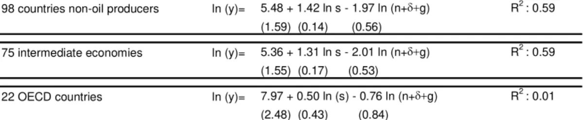
Using OLS (n and g are independent of the error term), MRW tested the
Solow model for 98 countries that are not oil producers, 75 countries with intermediate economies and 22 countries of the OECD. They excluded extremely small countries and also those with doubtful data. The data comes from the Real National Accounts (World Bank), comprising all economies except centrally planned economies in the period between 1960 and 1985.
As we can see in table 1, significance was found for the first two groups of countries, but the same did not happen for the 22 OECD countries. The values between brackets identify the standard errors (the other numbers are, of course, the estimated coefficients), which are, for the last group of countries, extremely small when compared with the values of the parameters in the first two sets of countries. This makes the coefficients of the OECD sample non-significant.
Table 1. Results of Mankiw et al.’s regression
98 countries non-oil producers ln (y)= 5.48 + 1.42 ln s - 1.97 ln (n+g) R2 : 0.59 (1.59) (0.14) (0.56)
75 intermediate economies ln (y)= 5.36 + 1.31 ln s - 2.01 ln (n+g) R2 : 0.59 (1.55) (0.17) (0.53)
22 OECD countries ln (y)= 7.97 + 0.50 ln (s) - 0.76 ln (n+g) R2 : 0.01 (2.48) (0.43) (0.84)
The independent variables explain 59% of the growth of the 98 countries
that are not oil producers (i.e. saving and population growth account for 59% of
the variation in income per capita), and the percentage is similar for the 75 intermediate economies. For the third sample (which is the smallest), the coefficients are not significant and the Solow model does not fit. Another
relevant result is that in the pure Solow version is higher (around 0.6) than
expected (the share of capital in income is between 0.25 and 0.4).
MRW tried to improve the Solow model adding it human capital. In fact, human capital had already been labelled by some economists as being very important in the process of growth. For example Kendrick (1976) estimated that more than half of the total U.S.A. capital stock in 1960 was human capital.
One of the first to include human capital in a growth model was Lucas (1988).
In the augmented version of the Solow model, MRW included that
stands for the proportion of human capital in the production function, which is:
1
L H K
Y (15)
The coefficients and range between 0 and 1, and +<1. Human
capital is the knowledge of the workers, which comes from investment in education, training, and self-teaching. As it happens to physical capital, human capital can depreciate as individuals inevitably die (or get severely injured), and we must keep in mind that certain skills can become lost with time due to sloppiness.
The authors assume that both physical and human capital depreciate at the same rate.
) ln( . 1 ln . 1 ln ). 1 ( ) 0 ( ln * ˆ
lny A sk sh ng
(16)
sk and sh are, the proportions of income invested in physical and human
capital.
As a proxy to human capital accumulation (sh) the authors use data of the
population enrolled in secondary school (aged 12 to 17), obtained from UNESCO.
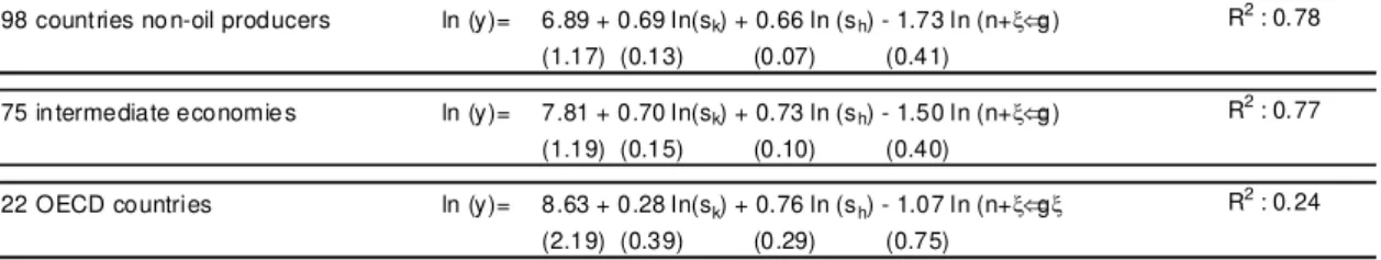
Table 2. Results of Mankiw et al.’s regression with human capital
98 countries no n-oil producers ln (y)= 6.89 + 0.69 ln(sk) + 0.66 ln (sh) - 1.73 ln (n+g) R 2
: 0.78 (1.17) (0.13) (0.07) (0.41)
75 in termediate economie s ln (y)= 7.81 + 0.70 ln(sk) + 0.73 ln (sh) - 1.50 ln (n+g) R 2
: 0.77 (1.19) (0.15) (0.10) (0.40)
22 OECD countries ln (y)= 8.63 + 0.28 ln(sk) + 0.76 ln (sh) - 1.07 ln (n+g R2 : 0.24 (2.19) (0.39) (0.29) (0.75)
SOURCE: Mankiw, N.G., Romer D., and Weil, D. (1992) A Contribution to the Empirics Growth, Quarterly Journal of Economics, 107, Table II, p.420
The inclusion of human capital proves to be an improvement to the model
with the investment (saving) rate, the log of (n++g) and the log of the
percentage of population in secondary school explaining nearly 80% of the cross-country variation in income per capita in the non-oil and intermediate samples.
and are about one third for the first two samples (the estimate for
OECD is not different but less precise), which is a much more expected result.
In the work of MRW, initial efficiency A(0) is unobserved and hence omitted, but if initial efficiency is correlated with the regressors then estimates will be biased. To solve this, Temple uses dummy variables for Sub-Saharan Africa, Latin America and the Caribbean, East Asia, and the set of industrialized countries.
Other problem identified by Temple is the assumption of identical rates of technical progress, which implies that income per capita will grow at the same rate in steady state. Lee, Pesaran and Smith (1997) had already demonstrated that this assumption led to biased estimates of convergence rates. However, this simplification proves to be useful and Temple maintains it.
When outliers are removed, Temple considers that the MRW model has no explanatory power for OECD countries. Measurement errors in initial income and in the conditioning variables cause problems in the estimated convergence rates. We will see this in detail in chapter 4.
Literature is fertile in suggesting methods to treat the problem of outliers, however Temple chose robust statistics. He applies Least Trimmed Squares (LTS) estimator, which works by minimizing the sum of squares over half the observations, picking the half with the smallest residual sum of squares. He also applied a procedure called Reweighted Least Squares (RWLS), which helps in tagging observations with high residuals as unrepresentative, since these are distant from the robustly fitted regression line.
The use of LTS on the OECD sample identifies 3 unrepresentative observations: Greece, Portugal and Turkey. When these last two countries are removed from the sample, the R-squared drops from 0.35 to 0.02 and the explanatory value of the augmented Solow model simply vanishes.
With the RWLS procedure, we can see that without outliers the augmented
Solow model holds, with the R-squaredsaround 0.6, as shows Table 3. There
are apparent problems. For example, the relation between per capita income and
population growth (the term in ln(n g)), has different coefficients
capturing that relation. However, differences across countries in technical
progress (g) and capital depreciation () could account for this.
Table 3. Temple’s robust regression estimates, by RWLS, stratified sample
Dependent variable: log GDP per working-age person in 1985
Quartile observations Poorest 20 Second 20 Third 20 Richest 20 Constant 7.64 11.9 8.20 8.39 (1.70) (1.98) (1.02) (1.03) ln (I/GDP) 0.18 0.04 0.44 0.32 (0.08) (0.24) (0.20) (0.25)
ln (n+g+δ) -0.15 1.17 -0.53 -0.90
(0.61) (0.81) (0.31) (0.28) ln (SCHOOL) 0.20 0.40 0.16 0.38 (0.06) (0.12) (0.16) (0.17)
R2 0.58 0.58 0.62 0.67
Restriction p-value 0.62 0.07 0.91 0.68 RESET p-value 0.97 0.82 0.80 0.14
Implied α 0.13 0.03 0.28 0.19
Implied β 0.14 0.28 0.10 0.22
Quartile Unrepresentative observations dropped in RWLS Poorest Botsw ana, Cameroon, Egypt, Indonesia, Zaire Second Brazil, Ghana, Korea, Papua New Guinea, Tunisia Third Hong Kong, Jamaica, Japan, Mexico, Singapore, Spain Richest Argentina, Chile, Ireland, Uruguay
Notes: MacKinnon-White (1985) HCSEs in parentheses. The technology parameters α and β
are calculated using the coefficients on ln (I/GDP) and ln (SCHOOL).
SOURCE: Temple, J. (1998) Robustness tests of the Augmented Solow Model, Journal of Applied Econometrics, 13, Table I, p.367.
The way Temple split the sample was inspired in Durlauf and Johnson’s work (1995). They divided the MRW sample using 1960’s income and literacy rates and argue that common technology is not a realistic assumption, since technology parameters vary across samples.
Table 4. Durlauf and Johnson’s Cross-section regressions: regression tree sample
breaks
Dependent variable: ln (Y/L)i, 1985 - ln (Y/L)i, 1960
1 2 3 4
Observations 14 34 27 21
Constant 3.46 -0.915 0.277 -7.26a
(2.27) (1.79) (1.42) (1.59) ln(Y/L)i,1960 -0.791
a
-0.086 -0.316a 0.069 (0.269) (0.131) (0.123) (0.139)
ln (I/Y)i 0.314
a
0.129 1.110a 0.475a (0.109) (0.159) (0.165) (0.119)
ln (n+g+δ)i -0.429 -0.390 0.059 -1.75
a
(0.678) (0.489) (0.451) (0.270)
ln (SCHOOL)i -0.028 0.469
a
-0.014 0.341a (0.073) (0.095) (0.167) (0.141)
0.57 0.52 0.57 0.82
σε 0.16 0.28 0.28 0.12
θ 4.107a 0.539 -3.95 -11.0
(0.552) (1.809) (2.67) (7.64)
α 0.306a 0.186 0.758a 0.333a
(0.083) (0.123) (0.095) (0.100)
γ -0.034 0.416a -0.073 0.455a
(0.083) (0.080) (0.114) (0.103)
0.64 0.40 0.55 0.71
σε 0.19 0.32 0.30 0.18
Terminal node number
Unconstrained regressions Constrained regressions 2 R 2 R
Note: a Significance at asymptotic 5% level.
SOURCE: Durlauf, S. N., and Johnson, P. A. (1995) Multiple Regimes and Cross-Country Growth Behavior, Journal of Applied Econometrics, 10, Table V, p.375.
While MRW’s unconstrained model explains 46% of the growth
variation1, we can see in the upper table, that this multiple regime model, for the
Different estimates of both physical and human capital shares across subsamples suggest that economies with unequal initial conditions have different aggregate production functions.
3.2.1 LEAMER’S SENSITIVITY ANALYSIS
Levine and Renelt (1992) were not convinced by the existing studies at their time and took specific measures to deal with the lack of adherence of the regression results to reality, which was caused by missing (the majority of investigators uses a small number of explanatory variables) or biased variables. Multicollinearity was also a reason for the aforementioned problem. Another criticism was that those who examine the impact of fiscal policy ignore trade policy and vice-versa.
For them, linkages between growth rate and sets of variables related to political, economic and institutional indicators based on cross-country regressions should be looked upon with caution.
These authors applied the sensitivity analysis suggested by Leamer (1983, 1985), which is the extreme-bound analysis (EBA). It tests the robustness of coefficient estimates to changes in the conditioning set of data.
The procedure consists in estimating the regression with all the independent variables, one at a time or in small groups, together with a focus variable. If we want to estimate the effect of trade in income per capita, then we could use a simple linear regression like:
d0 d1
y (international trade) (17)
d0 d1
y (international trade) d2X (18)
in which X is a variable or a group of variables. If d2remains with significance
and does not change sign in every regression, we can say that y is positively
related to trade and that the estimated coefficient is not accidentally selected through other variables included in the equation. In this case, international trade is robustly related with income per capita.
Levine and Renelt ran regressions for different focus variables and concluded that there are few variables with this characteristic (robustness). They aimed to prove that many popular cross-country growth findings are sensitive to the conditioning information set. In fact it is hard to isolate a strong empirical relationship between any particular macroeconomic policy indicator and long run growth.
Few of the relationships found in cross-country regressions escape from Levine and Renelt´s scrutiny. A positive and robust correlation between growth and the share of investment in GDP really exists and the ratio of trade to output is also robust and positively correlated with the investment share.
The authors state that only when we identify a significant correlation while controlling for other relevant variables, should we have much confidence in the correlations.
An objection to the EBA is the introduction of multicollinearity, which as we have seen before, changes the standard error of the coefficients. In order to minimize this, the authors apply a series of restrictions. Nevertheless, Leamer (1978) points out that the appearance of multicollinearity derives from a weak-data problem.
They use data from 119 countries, compiled from the World Bank, IMF and also other authors (Barro, Summers and Heston).
Originally, the EBA uses equations of the form:
I M Z
where y is either the GDP per capita growth or the share of investment in GDP,
I is a set of variables, M the variable of interest, Z a subset of variables chosen
from a group of variables (up to three) identified in past studies as important
explanatory variables of growth, and the error term.
For each model, one finds an estimate m and the standard deviation m.
The EBA test for variable M says that if the lower extreme bound is negative
and the upper extreme bound is positive, then variable M is not robust.
Table 5. Sensitivity analysis for basic variables
Dependent variable: growth rate of real per capita GDP, 1960-1989
M-variable Std.
Error t Countries R2 Other var.
Robust/f ragile
INV high: 19.07 2.87 6.66 98 0.54 STDI, REVC, GOV robust base: 17.49 2.68 6.53 101 0.46
low: 15.13 3.21 4.72 100 0.49 X, PI, REVC
RGDP60 high: -0.34 0.13 2.53 98 0.54 STDI, PI, GOV robust base: -0.35 0.14 2.52 101 0.46
low: -0.46 0.13 3.38 85 0.56 GD C, X, REVC
GPO high: -0.34 0.23 1.48 100 0.48 X, STDI, PI fragile base: -0.39 0.22 1.73 101 0.46
low: -0.49 0.20 2,42 85 0.56 X, GDC, REVC
SEC high: 3.71 1.22 3.04 84 0.55 X, GOV, GDC robust base: 3.17 1.29 2.46 101 0.46
low: 2.50 1.15 2.17 85 0.62 X, STDD, GD C β
Notes:The base is the estimated coefficient from the regression with the variable of interest (M-variable) and the always-included variables (I-variables). The I-variables, when the dependent variable is the growth rate of real per capita GDP, are INV (investment share of GDP), RGDP60 (real GDP per capita in 1960), GPO (growth in population), and SEC (secondary-school enrolment rate in 1960). The high is the estimated coefficient from the regression with the extreme high bound (m+two standard deviations); the low is the coefficient from the regression with the extreme lower bound. The "other variables" are the Z-variables included in the base regression that produce the extreme bounds. The robust/fragile designation indicates whether the variable of interest is robust or fragile. STDI – Standard Deviation of inflation; REVC – Number of revolutions and coups; GOV - Government Consumption share of GDP; X – Export share of GDP; PI – Average inflation of GDP deflator; GDC – Growth rate of domestic credit; STDD – Standard deviation of GDC.
SOURCE: Levine, R., and Renelt, D. (1992) A Sensitivity Analysis of Cross-Country Growth Regressions, The American Economic Review, 82, Table 1, p.947
The results above show that (in table 5 the dependent variable is the growth rate), the investment (INV) coefficient is positive and robust, thus validating previous studies. With RGDP60, we can see that poor countries tend
to grow faster than the rich ones (all other things equal), i.e., there is
However, other familiar correlations in cross-country regression about growth do not pass Levine and Renelt’s tests. For example population growth (GPO) is not clearly associated with the per capita growth.
They did the same considering investment share as the dependent variable, but none of the relationships were robust.
Table 6 below (again with the growth rate of real per capita GDP as the
dependent variable) shows that all tested correlations are fragile, i.e., none of
the fiscal-policy indicators are robustly correlated with growth rates.
Table 6. Sensitivity results for fiscal variables
Dependent variable: growth rate of real per capita GDP
M-variable (period) Std.
Error t Countries R2 Other var.
Robust/f ragile
GOV (1960-1989) high: -0.85 3.20 0.27 85 0.61 REVC, STDD , GDC fragile (0) base: -4.17 2.96 1.41 98 0.52
low: -5.52 3.33 1.66 85 0.57 X, PI, GDC
TEX (1974-1989) high: -1.22 2.22 0.55 75 0.45 X, STDD, GDC fragile (1) base: -5.03 2.05 2.46 85 0.36
low: -5.51 2.02 2.73 86 0.41 REVC, PI, STDI
GOVX (1974-1989) high: -12.95 7.81 1.66 64 0.48 X, STDD, STDI fragile (2) base: -21.96 5.64 3.90 74 0.43
low: -23.73 5.64 4.21 75 0.57 REVC, PI, STDI
DEF (1974-1989) high: 14.17 5.36 2.64 82 0.41 REVC, PI, STDI fragile (1) base: 15.45 4.90 3.16 82 0.40
low: 6.22 5.98 1.04 72 0.47 STD D, REVC , PI β
Notes: The base is the estimated coefficient from the regression with the variable of interest (M-variable) and the always-included variables (I-variables). The I-variables, when the dependent variable is the growth rate of real per capita GDP, are INV (investment share of GDP), RGDPxx (initial real GDP per capita), GPO (growth in population), and SEC or SED (initial secondary-school enrolment rate). The high is the estimated coefficient from the regression with the extreme high bound (m
+two standard deviations); the low is the coefficient from the regression with the extreme lower bound. M-variable definitions: GOV= government consumption share; TEX = total government expenditure; GOVX =government consumption share minus defense and educational expenditures; DEF = central government surplus/deficit as share.
The "other variables" are the 2-variables included in the base regression that produce the extreme bounds. The underlined variables are the minimum additional variables that make the coefficient of interest insignificant or change sign. The robust/fragile designation indicates whether the variable of interest is robust or fragile. If fragile, the column indicates how many additional variables need to be added before the variable is insignificant or of the wrong sign. A zero indicates that the coefficient is insignificant with only the I-variables included.
Check the notes in table 5 for the definition of the “other variables”.
SOURCE: Levine, R., and Renelt, D. (1992) A Sensitivity Analysis of Cross-Country Growth Regressions, The American Economic Review, 82, Table 6, p.951
allocation of resources. When using the investment share as the dependent variable some of the variables are positively and robustly correlated with it, as we can see in table 7.
Table 7. Sensitivity results for trade variables
Dependent variable: investment share
M-variable (period) ErrorStd. t Countries R2 Other var. Robust/fragile
X (1960-1989) high: 0.16 0.030 5.31 87 0.26 GDC, STDI robust base: 0.14 0.024 5.90 106 0.25
low: 0.09 0.024 3.90 101 0.35 GOV, REVC, STDI
LEAM1 (1974-1989) high: 0.15 0.055 2.68 40 0.20 DEF, STDD, GDC robust base: 0.15 0.043 3.40 50 0.19
low: 0.10 0.050 2.08 48 0.24 REVC, STDD
LEAM2 (1974-1989) high: 0.24 0.044 5.32 48 0.39 GOV, STDD robust base: 0.22 0.039 5.55 50 0.39
low: 0.18 0.041 4.30 52 0.46 REVC, PI, GOV
BMP (1960-1989) high: -0.0002 0.0001 1.58 79 0.19 GDC, GOV, REVC fragile (3) base: -0.0004 0.0001 4.54 95 0.18
low: -0.0004 0.0001 3.78 81 0.18 PI, STDD, GDC
RERDB (1974-1989) high: -0.0002 0.0002 0.96 52 0.07 DEF, REVC fragile (0) base: -0.0002 0.0002 1.12 63 0.02
low: -0.0003 0.0002 1.46 59 0.15 STDD, GDC β
Notes: The base is the estimated coefficient from the regression with the variable of interest (M-variable). When the dependent variable is the investment share, no I-variables are included. The high is the estimated coefficient from the regression with the extreme high bound (m + two standard deviations); the low is the coefficient from the regression with the extreme lower bound.
M-variable definitions: X = exports as percentage of GDP; LEAMl = Leamer's (1988) openness measure based on factor-adjusted trade; LEAM2 = Leamer's (1988) trade-distortion measure based on Heckscher-Ohlin deviations; BMP = black-market exchange-rate premium; RERDB = Dollar's (1992) real exchange-exchange-rate distortion for SH benchmark countries.
The "other variables" are the Z-variables included in the base regression that produce the extreme bounds. The underlined variables are the minimum additional variables that make the coefficient of interest insignificant or change sign. The robust/fragile designation indicates whether the variable of interest is robust or fragile. If fragile, the column indicates how many additional variables need to be added before the variable is insignificant or of the wrong sign. A zero indicates that the coefficient is insignificant with only the I-variables included.
DEF – Ratio of central-government deficit to GDP. Check the notes in table 5 for the definition of the “other variables”.
SOURCE: Levine, R., and Renelt, D. (1992) A Sensitivity Analysis of Cross-Country Growth Regressions, The
American Economic Review, 82, Table 9, p.955
When testing monetary and political indicators, all correlations are not robust except for the one between investment share and revolutions and coups. A country with less turmoil benefits from more investment in comparison with a country that has an unstable political environment.
- Positive and robust correlation between average growth rates and the average share of investment in GDP, and between the share of investment in GDP and the average share of trade in GDP.
- A great variety of trade policy measures were not robustly correlated
with growth when the equation included the investment share.
- A significant set of fiscal indicators are not correlated with growth or
investment share, and the same happens with a broad array of institutional indicators.
3.3 RUNNING MILLIONS OF REGRESSIONS
Sala-i-Martin (1997a) handled the sensitivity analysis in a different way. He stated that the Levine and Renelt’s tests are so powerful that no variable would survive to the significance permanence criteria (and in keeping the same sign), through successive regressions.
He analyses the entire distribution and not only the extreme bounds. Denying the pessimistic view of Levine and Renelt, Sala-i-Martin found that a large number of variables can be strongly related to growth.
This author states that one of the problems in economy growth theory is the inexistence of a consensus on what variables cause growth.
Another problem is the empirical estimation of these determinants. Questions like: “How do we measure human capital?” and “How do we compare degrees of corruption in the government?” between the countries, have not an easy answer.
When the economists run the regressions, they combine the various
variables but often find that a first variable is significant only when the
regression includes second and third variables, becoming non-significant only when a fourth variable is included.
Sala-i-Martin develops a less dogmatic approach. He looks at the whole
distribution of m. In order to proceed, Sala-i-Martin had to operate under two
different hypotheses about the normality of the distribution (firstly that it is normal, and secondly that it is not).
This leads to different ways of calculating the weighted average of the N estimated variances (there are N possible combinations of Z, and Z belongs to a vector of up to three variables taken from all the available variables).
Sala-i-Martin keeps the Levine and Renelt model specification, following them in the procedure that allows all the models to include 3 fixed variables
considered a priori to be important determinants of growth. Regressions have
always seven explanatory variables (three fixed variables, the tested variable and trios of the remaining 58 variables).
Sala-i-Martin chose 62 variables that supposedly explain growth. The selection was based upon availability for the first years of the sample period, and also by the inexistence of endogeneity problems.
Thereby, he tests the 62 variables found in literature, plus the growth rate of GDP. The only considered dependent variable is the average growth of rate per capita GDP between 1960 and 1992.
To choose the fixed variables, Sala-i-Martin demanded three properties: they had to be very common in the literature, they had to be evaluated in the
beginning of the period (1960), and they had to be robust (i.e. systematically
relevant in the regressions ran in the previous literature). Consequently, he selected the following variables: level of income in 1960, life expectancy in 1960 and the primary school enrolment in 1960.
Therefore, from the 62 variables, Sala-i-Martin, three are fixed and for each variable tested he combines the remaining 58 and hence he estimates 30 856 models (58!/3!*55!).
Sala-i-Martin concluded that from the 62 variables tested in one or more
statistical studies in the last years, 22 have positive or negative coefficients, i.e.,
Table 8. Variables with significance in Sala-i-Martin’s two million regressions
Dependent variable: growth
Independent variables Coefficient () Standard deviation
Equipment Investment 0.2175 0.0408 Number of Years Open Economy 0.0195 0.0042 Fraction of Confucian 0.0676 0.0149 Rule of law 0.0190 0.0049 Fraction of Muslim 0.0142 0.0035 Political rights -0.0026 0.0009 Latin American Dummy -0.0115 0.0029 Sub-Sahara African Dummy -0.0121 0.0032 Civil Liberties -0.0029 0.0010 Revolutions and Coups -0.0118 0.0045 Fraction of GDO in Mining 0.0353 0.0138 S.D. Black Market Premium -0.0290 0.0118 Primary Exports in 1970 -0.0140 0.0053 Degree of Capitalism 0.0018 0.0008
War Dummy -0.0056 0.0023
Non-Equipment Investment 0.0562 0.0242 Absolute Latitude 0.0002 0.0001 Exchange Rate D istortions -0.0590 0.0302 Fraction of Protestant -0.0129 0.0053 Fraction of Buddhist 0.0148 0.0076 Fraction of Catholic -0.0089 0.0034 Spanish Colony -0.0065 0.0032
SOURCE: Sala-i-Martin, X. (1997a), I just run two million regressions, American Economic Review, 87, Table 1, p. 181
Table 8 presents these variables and we can see that the environment in which the economy operates, the incentive structure that affects the individual behaviour, the level of competition and the market regulations by the government are to be taken in account in the process of economic growth.
Five of the variables that stand for religious beliefs (Buddhism, Catholicism, Confucianism, Protestantism and Islamism) are related to economic growth, but not all in the same way. Countries where Buddhism,
Confucianism and Islamism are predominant, grow quicker, ceteris paribus,
than those inhabited by Catholics and Protestants in majority. Variables of
political nature as the number of revolutions and coups d’ état, wars, political
and civic freedom and democracy have the expected signs.
Institutions related to international trade and financial system are also important. That can be understood by looking at the coefficient of variables like the number of years as an open economy and the black market premium.
Sturm and de Haan (2000) suggest a different approach. As we have seen before, Sala-i-Martin analyses the entire distribution, instead of analysing the extreme bounds of the estimates of a particular variable like Levine and Renelt did.
Sturm and de Haan state that in modelling cross-country growth models the first thing to do is to identify the outliers. They use the Least Median of Squares (LMS) estimator of Rousseeuw (1984, 1985) to identify outlying observations. Its basic principle is to fit the majority of the data. After that it is
possible to identify the outliers, i.e. those cases with big positive or negative
residuals. However this estimator is not adequate for inference. Rousseeuw (1984) suggested Reweighted Least Squares (RLS) to surpass this problem. For Sturm and de Haan this is a better procedure than the one Sala-i-Martin followed. So, variables insignificant to the LMS/RLS method are not significantly related to economic growth.
The LMS estimator can be written as
2 ,.., 1 ˆ
min i
n i
mediane
(20)
where ei is the residual of case i with respect to the LMS fit. The use of RLS
consists in putting weight zero if the observation is an outlier and one if otherwise. The resulting estimator is more efficient and gives the usual inferential output as t-statistics and R-squared.
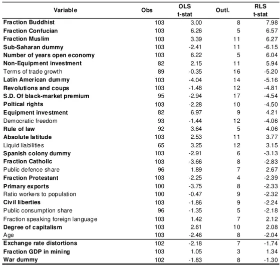
In the empirical analysis, Sturm and de Haan follow Sala-i-Martin. They use the same standard variables (level of income in 1960, life expectancy in 1960 and the primary-school enrolment rate in 1960). The sample has 103 countries, however data availability problems reduced it to only 65 in some cases.
growth according to Sala-i-Martin, but not for Sturm and Haan (bottom 3 of the table).
Table 9. Estimation results with OLS and RLS
Dependent variable: growth
OLS RLS
t-stat t-stat
Fraction Buddhist 103 3.00 8 7.98
Fraction Confucian 103 6.26 5 6.57
Fraction Muslim 103 3.39 11 6.27
Sub-Saharan dummy 103 -2.41 11 -6.15
Number of years open economy 103 6.22 5 6.04
Non-Equipm ent investment 82 2.15 11 5.94
Terms of trade growth 89 -0.35 16 -5.20
Latin American dum my 103 -4.04 14 -5.16
Revolutions and coups 103 -1.48 12 -4.81
S.D. Of black-market premium 95 -2.94 17 -4.54
Poltical rights 103 -2.28 10 -4.50
Equipment investment 82 6.97 9 4.21
Democratic freedom 93 -1.44 12 -4.06
Rule of law 92 3.64 5 4.06
Absolute latitude 103 2.53 11 3.77
Liquid liabilities 65 3.25 12 3.15
Spanish colony dummy 103 -2.91 6 -3.13
Fraction Catholic 103 -3.66 8 -2.83
Public defence share 96 1.89 7 2.67
Fraction Protestant 103 -2.25 4 -2.39
Primary exports 100 -3.75 8 -2.33
Ratio workers to population 100 -0.47 9 -2.32
Civil liberties 103 -1.86 9 -2.24
Public consumption share 96 -1.35 5 -2.18 Fraction speaking foreign language 103 1.42 7 2.12
Degree of capitalism 103 2.61 10 2.08
Age 103 -2.46 8 -2.04
Exchange rate distortions 102 -2.18 7 -1.74
Fraction GDP in mining 103 1.05 3 1.34
War dummy 102 -1.83 8 -1.30
Variable Obs Outl.
Note: Bold variables are found to be related to economic growth by Sala-i-Martin (1997a,b)
SOURCE: Sturm, J.E., and de Haan, J. (2000) No need to run millions of regressions, CESinfo Working Paper, No. 288, Table 1
The results obtained by both authors are similar. However, terms of trade growth is not significant according to Sala-i-Martin, while for Sturm and de Haan it is (this is the result of reweighting the outliers). The opposite happens for the war dummy. Removing the outliers turns it insignificant.
4. WHAT ABOUT CONVERGENCE?
Another issue that is frequently present in growth studies is convergence. It was Baumol (1986) who started this discussion. The appearance of Maddison (1992) and Summers and Heston’s (1993) data sets generated a vast literature on this subject. In simple terms, convergence is defined as the tendency of poor economies to grow more rapidly than rich economies. Mankiw (1995) wrote that finding convergence or not depends on the sample. If we have only homogenous economies then we have convergence, something that does not happen if the sample has diverse economies. According to the same author, the neoclassical model does not necessarily predict convergence. This only happens when countries are in the same steady state and have different initial conditions. If the steady states are different then the rich countries continue to be rich, and the poor countries remain poor.
4.1 CONDITIONAL CONVERGENCE AND σ AND β CONVERGENCE
At this point I have to introduce another concept, which is conditional convergence. As we have seen convergence takes place when we have a negative slope coefficient between the dependent variable (average GDP growth rate) and the explanatory variable (level of income). If we control the differences between the countries steady states and find a negative relation between growth rates and income levels, then we have conditional convergence. It exists in the neoclassical model because there is the prediction that each economy will converge to its own steady state (determined by saving and
population growth rates). Still we can divide convergence, in β convergence
(when poor economies grow faster than rich ones) and σ convergence (when the
dispersion per income or product decreases over time). For example, we have
conditional β-convergence when we run a cross-sectional regression on initial
Barro and Sala-i-Martin (1991) argue that β convergence matters when we want to know how fast and to what extent the per capita income of an economy will reach the average per capita of a group of economies. If we want to know
how was or will be the distribution of income across economies, the σ
convergence is the concept that is relevant.
4.1.1. EMPIRICAL STUDIES ON THE SUBJECT OF CONVERGENCE
In the following sections I will analyze the topic of convergence according to several empirical studies that are based on different approaches, namely cross-section regressions, panel data and quantile regression.
4.1.1.1CONVERGENCE ANDCROSS-SECTION REGRESSIONS
In the neoclassical model, income converges to its steady state level as follows:
)
( *
y y
y (21)
where (1)(ng).
λ is the speed at which the gap between the steady state level of capital and
its current level is closed and is usually known in the literature as the rate of convergence.
The majority of empirical studies point to a rate of conditional convergence of 2 percent per year, meaning that each country moves 2 percent closer to its own steady state each year.
Barro and Sala-i-Martin (1991) examined the existence of convergence in the U.S. states and also between regions of 7 different European countries. In
the first case, they worked with a sample from 1880 to 1988 and found a λ of
0.0175, very close to the aforementioned 2 percent a year. The inclusion of
regional dummies or sectoral variables plus regional dummies led to a similar λ,
although in the last case λ is stable across periods, something that did not
happen in the other specifications. However, the results proved the existence of
convergence in the sense that economies grow faster in per capita terms when they are further below the steady state position.
The dispersion of personal income across in the U.S.A. states, measured
by σ, also falls from 1880 (0.545) to 1988 (0.194). In this study, Barro and
Sala-i-Martin also trace the importance of government transfers payments, which obviously reduce the dispersion.
In the case of the European regions the results are similar.
In a subsequent paper, Barro and Sala-i-Martin (1992) try to evaluate if there is convergence between 98 countries and also between 20 OECD
countries. They find that there is convergence only in a conditional sense, i.e.,
only holding constant variables like initial school enrolment rates and the ratio of government consumption to GDP. Barro and Sala-i-Martin argue that the mobility of labour and technology speed up convergence.
Sala-i-Martin (1996) using a sample of regions of U.S., Japan, U.K., France, Italy, Spain and Canada confirms that the initial income per capita is
very important (check R-squared in the table below), and the λ is close to 2
Table 10. Sala-i-Martins’ regressions results
Countries
λ R2 λ R2
( s.e) ( s.e. R eg .) ( s.e) ( s.e. R eg .)
United States 0.017 0.89 0.022
-48 States (1880-1990) (0.002) [0.0015] (0.002)
-Japan 0.019 0.59 0.031
-47 Pref ectures (1955-1990) (0.004) [0.0027] (0.004)
-Europe Total 0.015 - 0.018
-90 regions (1950-19-90) (0.002) - (0.003)
-Germany 0.014 0.55 0.016
-(11 regions) (0.005) [0.0027] (0.006)
-UK 0.030 0.61 0.029
-(11 regions) (0.007) [0.0021] (0.009)
-France 0.016 0.55 0.015
-(21 regions) (0.004) [0.0022] (0.003)
-Italy 0.010 0.46 0.016
-(20 regions) (0.003) [0.0031] (0.003)
-Spain 0.023 0.63 0.019
-(17 regions) (1955-87) (0.007) [0.004] (0.005)
-Canada 0.024 0.29 -
-10 Provinces (1961-91) (0.008) [0.0025] -
-Long-run Panel Estimates Single regression
Note: The regression use nonlinear squares to estimate equations of the form (1/T)ln(yit / yi,t-T)=
=a-[ln( yi,t-T)](1-e-βT)(1/T)+”other variables”, where yi,t-T is the per capita income in region I at the beginning of the interval divided by the overall CPI. T is the length of the interval; “other variables” are regional dummies and sectoral variables that hold constant temporary shocks that may affect the performance of a region in a manner that is correlated with the initial level of income (recall that when the error term is correlated with the explanatory variable,
then the OLS estimate of λ is biased).
Each column contains four numbers. The first one is the estimate of λ. Underneath it, in parentheses, is standard error. To its right, the adjusted R2 of the regression and below the R2, the standard error of the equation. Thus,
constant, regional dummies and/or structural variables are not reported in the Table. The coefficients for Europe Total include one dummy for each of the eight countries.
Column 1 reports the panel estimates when all the subperiods are assumed to have the same coefficient λ. This estimation allows for time effects. For most countries, the restriction of λ being constant over the subperiods cannot be rejected (see Barro and Sala-i-Martin, 1995).
Column 2 reports the value of λ estimated from a single cross section using the longest available data. For example, for the United States, the coefficient λ estimated by regressing the average growth rate between 1880 and 1990 is
λ=0.022 (s.e.=0.0002).
SOURCE: Sala-i-Martin, X. (1996) Regional cohesion: Evidence and theories of regional growth and convergence, European Economic Review, 40, Table 1, p.1331
Studies with regional prices that reach the same λ, like the one by Shioji
spending more in the poor states. In his PhD dissertation (1990), Sala-i-Martin had already proved that results do not change despite government redistribution.
Mankiw et al. (1992) had found that unconditional convergence exists
only for the OECD countries. Temple (1998) confirms it and says that unrepresentative observations are irrelevant in this case.
When it comes down to conditional convergence, Temple argues that his methodology shows that the augmented Solow model explanation power is not as strong as one could think. For example, the population growth and schooling in the non-OECD samples are wrongly signed and are not significant, as we can see in the following table.
Table 11. Temple’s tests for conditional convergence: RWLS estimation
Dependent variable: log difference GDP per working-age person in 1960-1985
Sam ple observations
Non-oil 92 Intermediate 69 OECD 21 Non-oil, non-OECD 71 Interm ediate, non-OECD 50 Constant 3.82 3.50 1.34 4.37 4.18
(0.79) (0.75) (1.19) (1.14) (1.29) ln(Y60) -0.30 -0.30 -0.32 -0.23 -0.24 (0.06) (0.07) (0.07) (0.08) (0.10) ln (I/GDP) 0.59 0.66 0.13 0.56 0.61 (0.09) (0.12) (0.20) (0.10) (0.13)
ln (n+g+δ) -0.04 -0.24 -0.94 0.45 0.29
(0.24) (0.24) (0.29) (0.35) (0.43) ln (SCHOOL) -0.01 0.00 0.13 -0.07 -0.04 (0.06) (0.10) (0.17) (0.06) (0.10)
R2 0.71 0.75 0.74 0.70 0.72
Restriction p-value 0.05 0.13 0.05 0.01 0.05 Implied λ 0.014 0.014 0.015 0.010 0.011
Sample Unrepresentative observations dropped in RWLS Non-oil Chad, Chile, Hong Kong, Mauritania, Somalia, Zambia Intermediate Argentina, Cameroon, Chile, Hong Kong, India, Zambia
OECD Japan
Non-oil, non-OECD Cameroon, Chad, Papua New Guinea, Somalia, Zambia Intermediate, non-OECD Cameroon, Chile, Zambia
Note: MacKinnon-White (1985) HCSEs in parentheses.
SOURCE: Temple, J. (1998) Robustness tests of the Augmented Solow Model, Journal of Applied Econometrics, 13, Table II, p.368.