Visualizing Structures in Confocal Microscopy Datasets Through Clusterization: A
Case Study on Bile Ducts
Lizeth A. C. Beltran∗, Carolina U. Cruz†, Jorge Luiz dos Santos‡, Pranavkumar Shivakumar§, Jorge Bezerra§ and Carla M.D.S. Freitas∗
∗Federal Univ. of Rio Grande do Sul, Porto Alegre, Brazil, Email:[lacbeltran,carla]@inf.ufrgs.br †Hospital de Cl´ınicas de Porto Alegre, Porto Alegre, Brazil, Email: [email protected],
‡Universidade da Beira Interior, Portugal, Email: [email protected],
§Cincinnati Children’s Hospital, Cincinnati, USA, Email: [lpranav.shivakumar,jorge.bezerra]@cchmc.org
Abstract—Three-dimensional datasets from biological tissues
have increased with the evolution of confocal microscopy. Hep-atology researchers have used confocal microscopy for investi-gating the microanatomy of bile ducts. Bile ducts are complex tubular tissues consisting of many juxtaposed microstructures with distinct characteristics. Since confocal images are difficult to segment because of the noise introduced during the specimen preparation, traditional quantitative analyses used in medical datasets are difficult to perform on confocal microscopy data and require extensive user intervention. Thus, the visual explo-ration and analysis of bile ducts pose a challenge in hepatology research, requiring different methods. This paper investigates the application of unsupervised machine learning to extract relevant structures from confocal microscopy datasets repre-senting bile ducts. Our approach consists of pre-processing, clustering, and 3D visualization. For clustering, we explore the density-based spatial clustering for applications with noise (DBSCAN) algorithm, using gradient information for guiding the clustering. We obtained a better visualization of the most prominent vessels and internal structures.
Keywords-confocal microscopy data; image processing;
DB-SCAN clustering; volumetric visualization
I. INTRODUCTION
The confocal microscope has the ability to remove out-of-focus light and the capability of controlling the depth of field and collecting several aligned images of the same sample [1]. These characteristics have led to its increasing use for the acquisition of volumetric datasets from biological samples. In this work, we focus on the visualization of the bile ducts structure imaged with confocal fluorescence microscopy.
Bile ducts are thin tubular structures that carry the bile, and studying their microanatomy is a hot topic in hepatology research [2–4]. Usually, confocal microscopy images of bile ducts are studied by analyzing the serial slices obtained from fluorescent samples of mice. However, despite the effort dedicated to the samples preparation and the image acquisition itself, it still is necessary adequate computational support for the analysis and visualization of such confocal microscopy datasets. Bile ducts are mainly composed of two different groups of complex and juxtaposed microstructures (Fig.1): Microvasculature and Peribiliary glands (PBGs). The microvasculature refers to the network of small vessels
that surround the bile ducts [5]. PBGs are clusters of cells that elongate to form complex epithelial networks that course and branch within the bile duct walls [2]. The visual inspection of these structures is decisive to understand the development of biliary diseases associated with vascular disorders. However, there are some challenges to understand the characteristics of the microvasculature as well as PBGs because of their complex morphology, induced by their shapes and overlapping. Furthermore, confocal microscopy images are affected by the noise introduced due to the specimen preparation process, such as the procedure of staining [6].
In this paper, we propose an exploratory approach to detect, identify and visualize clusters of voxels that rep-resent similar structures in bile ducts confocal microscopy datasets. We adopt clustering by the Density-Based Spatial Clustering DBSCAN algorithm, which creates clusters with arbitrary shapes, even in the presence of noise in large spatial databases [7]. To the best of our knowledge, there is no reported application of this technique in the study of data from hepatological samples. Our work aims at adapting the DBSCAN method for extracting structures from confocal images of bile ducts. The main challenge is to find the appropriate similarity features between voxels that allow for differentiating such structures. The main contributions of this work are the use of gradient information as a feature to guide the clustering process and the proposal of a specific pre-processing step that can also be used in other applications involving confocal microscopy images.
II. BACKGROUND AND RELATED WORK Confocal microscopes produce multichannel fluorescent datasets in which each channel is collected separately [1]. Confocal images are affected by some artifacts and noise, and irrelevant structures may also be labeled through the fluorescent staining process, resulting in visual occluders [8]. Regarding hepatology research, we found a few works us-ing confocal microscopy to study the micro-anatomy of bile ducts. DiPaola et al. [2] identified peribiliary glands (PBGs) residing within the bile duct walls. However, the images 2019 IEEE 32nd International Symposium on Computer-Based Medical Systems (CBMS)
(a) Red channel (b) Green channel (c) Superimposed channels
Figure 1: View of a single slice from a bile duct dataset: (a) the red channel encodes the microvasculature, while (b) the green one encodes the peribiliary glands. The dataset has 192 slices (512 x 512 image each)≈ 50 millions of points.
were visualized using the confocal microscopy proprietary software, which provided limited features for image post-processing. Hammad et al. [3] and Vartak et al. [4] used confocal microscopy to visualize intrahepatic bile ducts that are much smaller than the extrahepatic bile ducts we work with.
In a previous work [9], we proposed a pipeline to enhance and visualize the microvasculature of bile ducts. The pipeline consists of a non-linear filtering step and direct volume rendering. However, direct volume rendering requires the design of transfer functions, which are difficult to create for noisy data. In our previous work, transfer functions were obtained by a trial and error process.
In this paper, we also adopt direct volume rendering for displaying the clusters containing the structures of interest, with transfer functions based on the voxel values that char-acterize the clusters. Since the clustering method minimizes noise points, transfer functions are easier to design.
Clustering plays an important role in the fields of knowl-edge discovery and data mining [10]. Since our approach is exploratory, and we do not know a priori the number of clusters to partitioning the data, we decided to focus on density-based algorithms. The density-based clustering algorithm known as Density-Based Spatial Clustering of Applications with Noise (DBSCAN) [7] discovers clusters of arbitrary shapes and is based on two global parameters: eps, which is the radius around a pixel for the density calculation, i.e., the size of the eps neighborhood, and minPts that corresponds to the minimum number of points required to form a cluster.
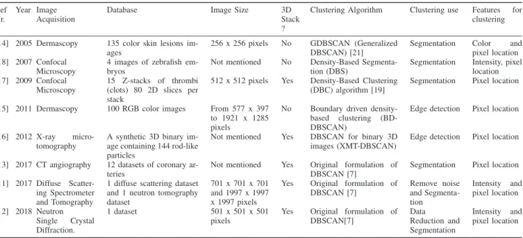
DBSCAN has been successfully applied in images datasets obtained from different sources for application in distinct domains [11–16], including confocal images [17, 18]. Table I summarizes the main characteristics of these works. Due to space constraints, we restrain ourselves to give details about those works related to the use of density-based clustering in images from confocal microscopy. Mu et al. report that the density-based spatial clustering approach
is useful for image segmentation of blood thrombus [17]. Mu et al. did not use DBSCAN, but a generalized version of the density-based clustering proposed by Chen et al. [19]. Chan et al. also modified a different density-based clustering method, known as DENCLUE [20], to perform segmentation in confocal images to study gene expression on zebrafish [18]. The original method is based on a set of density distribution functions, which are, in fact, influence functions that model the influence of a given data point in its neighborhood. In Chan et al., the Density-Based Segmentation (DBS) method the density function of each pixel is calculated using the differences of pixel intensity with the neighboring pixels, which is an approximation of the gradient of each pixel like we did in our approach.
From all the surveyed papers that use the DBSCAN method, two features are used to guide the clustering: pixel location and intensity. In our work, in addition to the spatial position and the size of the neighborhood of the voxel, we also use its gradient magnitude to guide the clustering. III. DISCOVERING STRUCTURES IN BILE DUCTS
IMAGES
In hepatology research, the a priori labels (ground truth) on the pixels are not available. Creating labels by hand is a hard task due to the complexity of the structures and the high dimensionality of data. Thus, we formulate our problem of extracting structures from these data sets as a clustering problem.
The input datasets that we use in this work were acquired at the Cincinnati Children’s Hospital [2]. The mice bile duct was stained with two different fluorescent antibodies, α-tubulin and Cytokeratin CK, to mark different tissues. The resulting dataset consists of two channels: the first one (red channel) represents the microvasculature or blood vessels around the bile duct with (α-tubulin staining) (Fig.1a); the second one (green channel) represents the bile duct wall containing the peribiliary glands with CK staining (Fig.1b). In the remainder of this section, we explain our approach
Table I: Summary of papers reporting density-based clustering in image datasets. Ref
Nr.
Year Image Acquisition
Database Image Size 3D
Stack ?
Clustering Algorithm Clustering use Features for clustering [14] 2005 Dermascopy 135 color skin lesions
im-ages
256 x 256 pixels No GDBSCAN (Generalized DBSCAN) [21]
Segmentation Color and pixel location [18] 2007 Confocal
Microscopy
4 images of zebrafish em-bryos
Not mentioned No Density-Based Segmenta-tion (DBS)
Segmentation Intensity, pixel location [17] 2009 Confocal
Microscopy
15 Z-stacks of thrombi (clots) 80 2D slices per stack
512 x 512 pixels Yes Density-Based Clustering (DBC) algorithm [19]
Segmentation Pixel location
[15] 2011 Dermascopy 100 RGB color images From 577 x 397 to 1921 x 1285 pixels
No Boundary driven density-based clustering (BD-DBSCAN)
Edge detection Pixel location
[16] 2012 X-ray micro-tomography
A synthetic 3D binary im-age containing 144 rod-like particles
Not mentioned Yes DBSCAN for binary 3D images (XMT-DBSCAN)
Edge detection Pixel location
[13] 2017 CT angiography 12 datasets of coronary ar-teries
Not mentioned Yes Original formulation of DBSCAN [7]
Segmentation Pixel location [11] 2017 Diffuse
Scatter-ing Spectrometer and Tomography
1 diffuse scattering dataset and 1 neutron tomography dataset
701 x 701 x 701 and 1997 x 1997 x 1997 pixels
Yes Original formulation of DBSCAN [7] Remove noise and Segmenta-tion Intensity and pixel location [12] 2018 Neutron Single Crystal Diffraction. 1 dataset 501 x 501 x 501 pixels
Yes Original formulation of DBSCAN[7] Data Reduction and Segmentation Intensity and pixel location
constituted by a pre-processing phase, the clustering to isolate structures and visualization.
A. Pre-processing
We use two operations to normalize the image stacks and prepare the data for the clustering process.
• Normalization: We apply contrast stretching to increase the visibility of the structures.
• Data Reduction: We remove all points with intensity 0 (background), for eliminating unnecessary points and reducing the amount of data that will undergo the clustering phase.
B. Density-Based Spatial Clustering
The spatial information, i.e., the coordinates (x,y,z) are a typical candidate clustering feature. As for images, any kind of pixel (or voxel) attribute can be used as a clustering feature. Confocal images have an inhomogeneous intensity inherent to the fluorescent staining process [22], and the gradient was investigated as a more robust candidate feature. After experimenting with the intensity and gradient values, we found out that the gradient was a richer source of information for distinguishing the regions of interest. Then, we adopted the gradient magnitude to guide the clustering process.
1) Determining the parameters for 3D clustering: In the original DBSCAN algorithm [7], the key idea is that, for each point of a cluster, the neighborhood defined by a given radius (eps) around it has to contain at least a minimum number of points (minPts), i.e., the local density in the neighborhood has to exceed some threshold. Based on some heuristics we determined the appropriate eps parameter, and
set minPts empirically. In the following, we give details about the configuration of DBSCAN for clusterizing our dataset.
The eps-neighborhood of a point dictates the maximum distance (radius) between two points for them to reside in the same neighborhood. A general heuristic to establish the value for eps is by computing the k-nearest neighbor distances. However, in a recent application of DBSCAN [11], a simplified calculation for eps was proposed. The author’s idea is that the coordinates of the data points in the case of 3D image datasets are uniformly distributed voxels. Then, it is possible to use the Cartesian coordinate system and Euclidean distance to obtain the neighborhood. Values of eps in the interval [1,√2] includes the six first nearest neighbors, values in [√2,√3] to include the twelve second nearest neighbors, and so on. Based on this last approach, we fixed the eps to 1.7≈ (√7). This value means that the local density function uses 18 nearest neighbors of a given point data in the clustering.
minPts denotes the minimum number of points located in an eps-neighborhood, and is data dependent. If we select a low minPts value, we get more clusters from noise. We have experimented minPts values from 50 to 300, and finally set it to 200 points for the green channel and 50 points for the red channel.
The density in a neighborhood is just the sum of the weights of the points inside the neighborhood. By default, each data point has weights 1, so the density estimate for the neighborhood is just the number of data points inside the neighborhood. We can use the parameter weight to change the importance of points [23]. The weight is an optional
(a) Original Volume (b) Cluster 1 (c) Clusters 2 to 2478
Figure 2: 3D visualization of the microvasculature of a bile duct: points shown in (b) represent the most prominent vessels extracted as cluster 1, and those shown in (c) are considered noise and were detected as clusters 2 to 2478. The color associated to the data points maps the depth of the data points.
parameter to perform clustering based on a specific feature. As described before, we have chosen the gradient magni-tude as a feature to guide the clustering. We follow the model for the weight parameter proposed by [11]. However, we use the gradient magnitude instead of intensity. We calculate the gradient magnitude for every point of the dataset considering the x, y, and z dimensions. Then, we take a specific value of gradient magnitude as a threshold. We fixed the threshold empirically as 20 for the red and the green channel. Any data point with gradient magnitude less than the threshold will take the weight of 1, while the data points with gradient magnitude greater than the threshold will have their weights assigned to the difference between their gradient magnitude and the threshold.
2) DBSCAN applied to 3D data points using gradient information: We used the DBSCAN R package [23] to perform the clustering on the 3D data points. As mentioned before, we configured the eps and minPts parameters and feed the algorithm with a list of data points containing their x, y, and z coordinates and the weight obtained from the gra-dient information. It is important to recall that background voxels are not considered in the clustering phase (refer to Section III-A). In this way, the clustering method uses both information (gradient and spatial location) to obtain at least the minPts data points for each cluster. The output is the list of points labeled with the cluster identification of each point as well as basic numbers about the clusters detected. Then, we use the original volumetric dataset again, and voxels belonging to the cluster of interest form a new volume that is passed to the visualization module.
IV. RESULTS AND DISCUSSION A. Microvasculature: Red Channel
Figure 2 shows 3D visualizations of selected regions in the dataset that contain the microvasculature (red channel)
of the bile duct. We obtained a total of 2478 clusters from the clustering process in the red channel. Due to the large number of clusters detected by DBSCAN, we summarize the results in the plot shown in Figure 4a, and use it to select the clusters for 3D visualization. Figure 2a shows the original dataset rendered with direct volume rendering. We identified most of the points as belonging to clusters 0 and 1. The cluster 0 is composed by 250,081 noise points, which can be discarded for visualization and analyses purposes. In other words, cluster 0 contains all the points that do not satisfy the conditions to belong to a cluster. Since clusters 1 to 2478 represent the detected objects, and cluster 1 is the largest one among them representing a connected region, it is the one that best represents the microvasculature (Figure 2b). Figure 4a shows that the clusters 2 to 2478 contain a lower quantity of points, and so we can also consider these points as noise (Figure 2c).
B. Peribiliary Glands (PBGs): Green Channel
In the case of the green channel, we obtained a total of 3,603 clusters (more clusters than in the red channel). In this case DBSCAN detected 1,998,026 noise points. Figure 3 shows the 3D visualization of data points belonging to clusters chosen among the ones that were detected in the green channel dataset. As we did in the processing of the red channel, we summarized the DBSCAN result in a plot (Figure 4b) that allowed us to analyze and select for visu-alization only the relevant clusters. Cluster 0 corresponds to the noise points. For the other clusters, we find a behavior similar to the red channel: cluster 1 is the most prominent one, representing a connected region containing the internal bile duct wall and the peribiliary glands. The other clusters, i.e., clusters 2 to 3,603, contain a lower quantity of points, and we can also consider them as noise. While Figure 3a shows the original volume, cluster 1 representing the internal
(a) Original Volume (b) Cluster 1 (c) Clusters 2 to 3,603
Figure 3: 3D visualization of the bile duct wall and PBGs: points shown in (b) represent mostly the PBGs identified as cluster 1, and those shown in (c) are also considered noise and were detected as clusters 2 to 3,603.
bile duct wall and the PBGs are presented in Figure 3b. Figure 3c present the clusters[2−3603], considered as noise.
0 500000 1000000 1500000 2000000 2500000 0 500 1000 1500 2000 2500
Points per Cluster
Cluster Index
(a) Red channel
0 1000000 2000000 3000000 4000000
0
1000
2000
3000
Points per Cluster
Cluster Index
(b) Green channel
Figure 4: Number of points detected per cluster.
C. Discussion
When comparing our work to others that adapt DBSCAN for their application domain, we found different approaches. For example, Celebi et al. used the original DBSCAN method for segmenting 2D digital images of skin lesions [14], while Tran et al. presented a version of DBSCAN to process 3D binary images, using the coordinates of the original image data and solving a known instability issue of the original DBSCAN in classifying border points of adjacent objects [16]. Our method is not limited to binary images and also uses the original data points’ coordinates.
Regarding the use of additional features to guide cluster-ing with DBSCAN, only two works adopt this approach. Hui and collaborators [11, 12] use the intensity value as a feature for selecting the points during the clustering. In our work, besides the spatial position and the size of the neighborhood, we use the gradient information to select the points during the clustering.
V. FINAL COMMENTS
In this paper, we have studied the DBSCAN method to extract relevant structures from confocal microscopy images of bile ducts. Our images can be divided into two different datasets, each one representing a separate channel that encodes distinct, but hard to visualize structures: the microvasculature, in the red channel, and the bile duct wall and peribiliary glands, in the green channel.
Aiming at a better result from previous works, we em-ployed some heuristics found in the literature to determine the appropriate parameters for the clustering. We proposed our methodology by adding some steps to be performed before the clustering phase: one step for pre-processing the volumetric dataset and another to analyzing candidate features to guide the clustering. In this latter aspect, we provide an interesting contribution: we have explored the gradient magnitude as a feature that allowed to extract rel-evant information from the density-based spatial clustering. Besides the fact that DBSCAN allows easy detection of noise points, an interesting result for both datasets was that the first and largest cluster found as significant for the visualization represents the structure of interest. In the red channel, this cluster represents the most prominent vessels, while in the green channel, the peribiliary glands were made more evident.
As future work, we want to explore multidimensional features to continue the search for better discriminating peri-biliary glands from the internal bile duct wall. Also, since we are interested in analyzing the peribiliary glands and the more prominent vessels, we will work on quantitative and qualitative measures for such structures.
Acknowledgments: We are grateful to the national re-search funding agencies CNPq (National Council for Scien-tific and Technological Development) and CAPES (CAPES Foundation, Finance Code 001) for financial support.
REFERENCES
[1] R. L. Price and W. G. Jerome, Basic Confocal Mi-croscopy. New York: Springer, 2011.
[2] F. DiPaola, P. Shivakumar, J. Pfister, S. Walters, G. Sabla, and J. A. Bezerra, “Identification of intramu-ral epithelial networks linked to peribiliary glands that express progenitor cell markers and proliferate after injury in mice,” Hepatology, vol. 58, no. 4, pp. 1486– 1496, 2013.
[3] S. Hammad, S. Hoehme, A. Friebel, I. Von Reck-linghausen, A. Othman, B. Begher-Tibbe, R. Reif, P. Godoy, T. Johann, A. Vartak et al., “Protocols for staining of bile canalicular and sinusoidal networks of human, mouse and pig livers, three-dimensional reconstruction and quantification of tissue microarchi-tecture by image processing and analysis,” Archives of toxicology, vol. 88, no. 5, pp. 1161–1183, 2014. [4] N. Vartak, A. Damle-Vartak, B. Richter, O. Dirsch,
U. Dahmen, S. Hammad, and J. G. Hengstler, “Cholestasis-induced adaptive remodeling of interlob-ular bile ducts,” Hepatology, 2016.
[5] K. Washington, P.-A. Clavien, and P. Killenberg, “Peri-biliary vascular plexus in primary sclerosing cholangi-tis and primary biliary cirrhosis,” Human pathology, vol. 28, no. 7, pp. 791–795, 1997.
[6] Y.-C. Chen, Y.-C. Chen, and A.-S. Chiang, “Template-driven segmentation of confocal microscopy images,” Computer Methods and Programs in Biomedicine, vol. 89, no. 3, pp. 239 – 247, 2008.
[7] M. Ester, H.-P. Kriegel, J. Sander, X. Xu et al., “A density-based algorithm for discovering clusters in large spatial databases with noise.” in Proceedings of the Second International Conference on Knowledge Discovery and Data Mining, vol. 96. AAAI Press, 1996, pp. 226–231.
[8] Y. Wan, H. Otsuna, C.-B. Chien, and C. Hansen, “An interactive visualization tool for multi-channel confocal microscopy data in neurobiology research,” Visualiza-tion and Computer Graphics, IEEE TransacVisualiza-tions on, vol. 15, no. 6, pp. 1489–1496, 2009.
[9] L. A. Beltran, J. L. dos Santos, C. U. Cruzz, and C. M. Freitas, “Enhancing the visualization of the microvasculature of extrahepatic bile ducts obtained from confocal microscopy images,” in Graphics, Pat-terns and Images (SIBGRAPI), 2016 29th SIBGRAPI Conference on. IEEE, 2016, pp. 25–31.
[10] R. Mehmood, G. Zhang, R. Bie, H. Dawood, and H. Ahmad, “Clustering by fast search and find of density peaks via heat diffusion,” Neurocomputing, vol. 208, pp. 210–217, 2016.
[11] Y. Hui and Y. Liu, “Volumetric data exploration with machine learning-aided visualization in neutron sci-ence,” arXiv preprint arXiv:1710.05994, 2017.
[12] Y. Hui, Y. Liu, and B.-H. Park, “Discovering features in sr {14} cu {24} o {41} neutron single crystal diffraction data by cluster analysis,” arXiv preprint arXiv:1809.05039, 2018.
[13] Z. Li, Y. Zhang, H. Gong, G. Liu, W. Li, and X. Tang, “An automatic and efficient coronary arteries extrac-tion method in ct angiographies,” Biomedical Signal Processing and Control, vol. 36, pp. 221–233, 2017. [14] M. E. Celebi, Y. A. Aslandogan, and P. R. Bergstresser,
“Mining biomedical images with density-based cluster-ing,” in Information Technology: Coding and Comput-ing, 2005. ITCC 2005. International Conference on, vol. 1. IEEE, 2005, pp. 163–168.
[15] M. Mete, S. Kockara, and K. Aydin, “Fast density-based lesion detection in dermoscopy images,” Com-puterized Medical Imaging and Graphics, vol. 35, no. 2, pp. 128–136, 2011.
[16] T. N. Tran, T. T. Nguyen, T. A. Willemsz, G. van Kessel, H. W. Frijlink, and K. van der Voort Maarschalk, “A density-based segmentation for 3d images, an application for x-ray micro-tomography,” Analytica chimica acta, vol. 725, pp. 14–21, 2012. [17] J. Mu, X. Liu, M. M. Kamocka, Z. Xu, M. S. Alber,
E. D. Rosen, and D. Z. Chen, “Segmentation, recon-struction, and analysis of blood thrombus formation in 3d 2-photon microscopy images,” EURASIP Journal on Advances in Signal Processing, vol. 2010, no. 1, p. 147216, 2009.
[18] P. Chan, S. H. Cheng, and T.-C. Poon, “Automated seg-mentation in confocal images using a density clustering method,” Journal of Electronic Imaging, vol. 16, no. 4, p. 043003, 2007.
[19] D. Chen, M. Smid, and B. Xu, “Geometric algo-rithms for density-based data clustering,” International Journal of Computational Geometry & Applications, vol. 15, no. 03, pp. 239–260, 2005.
[20] A. Hinneburg and D. A. Keim, “An efficient approach to clustering in large multimedia databases with noise,” in Proceedings of the Fourth International Confer-ence on Knowledge Discovery and Data Mining, ser. KDD’98. AAAI Press, 1998, pp. 58–65.
[21] J. Sander, M. Ester, H.-P. Kriegel, and X. Xu, “Density-based clustering in spatial databases: The algorithm gdbscan and its applications,” Data mining and knowl-edge discovery, vol. 2, no. 2, pp. 169–194, 1998. [22] J. Toriwaki and H. Yoshida, Fundamental of Three
Dimensional Digital Image Processing. New York: Springer, 2009.
[23] M. Hahsler, M. Piekenbrock, and D. Doran, “dbscan: Fast density-based clustering with r,” Journal of Sta-tistical Software, vol. 25, pp. 409–416.