A DIseAse MOdule Detection (DIAMOnD)
Algorithm Derived from a Systematic
Analysis of Connectivity Patterns of Disease
Proteins in the Human Interactome
Susan Dina Ghiassian1,2☯, Jörg Menche1,2,3☯, Albert-László Barabási1,2,3,4 *
1Center for Complex Networks Research and Department of Physics, Northeastern University, Boston, Massachusetts, United States of America,2Center for Cancer Systems Biology (CCSB) and Department of Cancer Biology, Dana-Farber Cancer Institute, Boston, Massachusetts, United States of America,3Center for Network Science, Central European University, Budapest, Hungary,4Channing Division of Network Medicine, Department of Medicine, Brigham and Women’s Hospital, Harvard Medical School, Boston, Massachusetts, United States of America
☯These authors contributed equally to this work. *[email protected]
Abstract
The observation that disease associated proteins often interact with each other has fueled the development of network-based approaches to elucidate the molecular mechanisms of human disease. Such approaches build on the assumption that protein interaction networks can be viewed as maps in which diseases can be identified with localized perturbation with-in a certawith-in neighborhood. The identification of these neighborhoods, ordisease modules, is therefore a prerequisite of a detailed investigation of a particular pathophenotype. While numerous heuristic methods exist that successfully pinpoint disease associated modules, the basic underlying connectivity patterns remain largely unexplored. In this work we aim to fill this gap by analyzing the network properties of a comprehensive corpus of 70 complex diseases. We find that disease associated proteins do not reside within locally dense com-munities and instead identifyconnectivity significanceas the most predictive quantity. This quantity inspires the design of a novel Disease Module Detection (DIAMOnD) algorithm to identify the full disease module around a set of known disease proteins. We study the per-formance of the algorithm using well-controlled synthetic data and systematically validate the identified neighborhoods for a large corpus of diseases.
Author Summary
Diseases are rarely the result of an abnormality in a single gene, but involve a whole cas-cade of interactions between several cellular processes. To disentangle these complex inter-actions it is necessary to study genotype-phenotype relationships in the context of protein-protein interaction networks. Our analysis of 70 diseases shows that disease protein-proteins are OPEN ACCESS
Citation:Ghiassian SD, Menche J, Barabási A-L (2015) A DIseAse MOdule Detection (DIAMOnD) Algorithm Derived from a Systematic Analysis of Connectivity Patterns of Disease Proteins in the Human Interactome. PLoS Comput Biol 11(4): e1004120. doi:10.1371/journal.pcbi.1004120
Editor:Andrey Rzhetsky, University of Chicago, UNITED STATES
Received:August 25, 2014
Accepted:January 9, 2015
Published:April 8, 2015
Copyright:© 2015 Ghiassian et al. This is an open access article distributed under the terms of the
Creative Commons Attribution License, which permits unrestricted use, distribution, and reproduction in any medium, provided the original author and source are credited.
Data Availability Statement:Data and source code for the DIAMOnD algorithm are within the Supporting Information files and can also be downloaded from
https://github.com/barabasilab/DIAMOnD. An interactive web-based version of the DIAMOnD algorithm is available athttp://diamond.barabasilab. com/.
not randomly scattered within these networks, but agglomerate in specific regions, sug-gesting the existence of specificdisease modulesfor each disease. The identification of these modules is the first step towards elucidating the biological mechanisms of a disease or for a targeted search of drug targets. We present a systematic analysis of the connectivi-ty patterns of disease proteins and determine the most predictive topological properconnectivi-ty for their identification. This allows us to rationally design a reliable and efficient Disease Mod-ule Detection algorithm (DIAMOnD).
Introduction
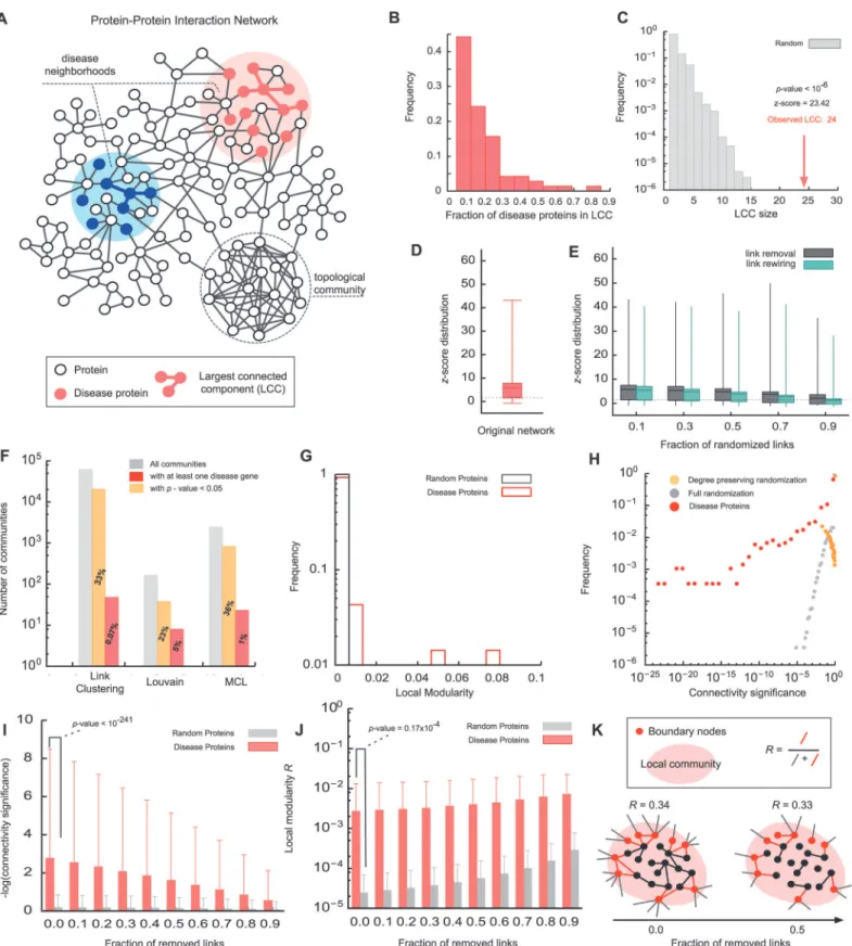
In the recent years, there is increasing evidence that proteins associated with a particular dis-ease have distinct interactions within theHuman Interactome, representing the cellular net-work of all physical molecular interactions [1–7]. The pathobiological properties of a disease and its clinical manifestations can be linked to perturbations within these disease neighbor-hoods, ordisease modules[8]. With recent advances in genome-wide disease gene association [9] and high-throughput Interactome mapping [10] we can already pinpoint the approximate location for some disease modules (Fig. 1A). For many diseases, however, a considerable frac-tion of their disease associafrac-tions remain unknown [11]. In this paper, we propose a network-based methodology to uncover the disease module associated with a particular phenotype. The algorithm is based on a systematic analysis of the network properties of known disease proteins across 70 diseases, revealing that instead of connectiondensitythe connectivitysignificanceis the most predictive quantity characterizing their interaction patterns. This quantity allows us to systematically explore the local network neighborhood around a given set of known disease proteins, helping us identifying promising new disease protein candidates.
Results
Interaction patterns of disease proteins within the Interactome
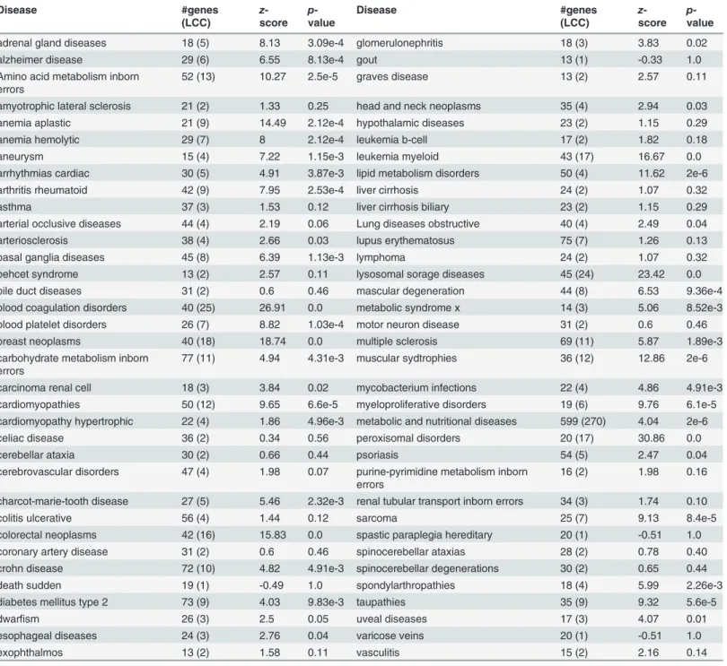
We started by compiling a comprehensive list of experimentally documented molecular inter-actions in human cells as described in [12] (seeMethods). We also curated a list of 70 well-characterized complex diseases (Table 1) and their known associated proteins from OMIM [13] and GWAS [9] (seeMethods). In total, we obtained 141,296 interactions between 13,460 proteins, 1,531 of which are associated with one or more diseases. Examining the subgraphs consisting of proteins associated with the same disease, we found that the largest connected component (LCC) typically contains only 10%-30% of the disease proteins (Fig. 1B). This sur-prisingly low fraction has been shown to be a direct consequence of the incompleteness of cur-rently available interactome maps [12]. Yet, despite this apparent scattering, the observed agglomeration is typically still higher than expected for randomly distributed proteins (Fig. 1C). The LCCs of 49 (out of 70) diseases are significantly larger (z-score>1.6) than ran-dom expectation (Fig. 1D,Table 1). To explore the possible influence of noise in the underlying Interactome on the observed clustering we repeated the analysis on perturbed networks with varying degrees of noise and incompleteness (seeMethods).Fig. 1Eshows that*50% of all diseases exhibit significant LCCs even after removing or randomizing up to 90% of the links in the network, indicating that the finding that disease proteins tend to reside in specific network neighborhood is remarkably robust.
From a network science perspective, the task of identifying these disease neighborhoods can be considered acommunity detectionproblem. Numerous algorithms [14–23] define a
10001771). The funders had no role in study design, data collection and analysis, decision to publish, or preparation of the manuscript.
community as a locally dense subgraph in a network (Fig. 1A). In order to evaluate the extent to which such topological community detection algorithms can be used to predict disease mod-ules, we chose three representative, methodologically distinct algorithms that have been suc-cessfully applied to identify communities of functionally related proteins (functionalmodules) in protein interaction networks:(i)A link community algorithm [14], which is based on link-similarities and can also capture hierarchical communities,(ii)the Louvain method, which max-imizes a global modularity function [21], and(iii)the Markov Cluster Algorithm (MCL), which detects dense regions based on random flow [24]. Each of these methods identifies a large num-ber of communities within the Interactome (Figs.1F&S1A-C). In order to evaluate whether some of these communities may be candidates for specific disease modules, we determined their enrichment with known disease proteins. We found that only between*1%-5% of the commu-nities detected by the different methods are significantly enriched (p-value<0.05, Fisher’s exact test) with any set of disease proteins (Fig. 1F). Conversely, only 15% of the diseases have any sig-nificantly enriched community. As these sigsig-nificantly enriched communities cover only* 15%-38% of all proteins associated with the respective disease, we were unable to assign for any of these diseases a single connected disease module (S1 Fig.D-F).
These results suggest that while topological communities may often represent meaningful
functional modules [25],they are not able to capturedisease modules. One possible reason for
this may be that disease proteins do not constitute particularly dense subgraphs. To further quantify this, we consider the modularity parameterR[23], a key measure used in community detection, whereR= 1 corresponds to perfect modularity andR*0 to randomly assigned com-munities (seeMaterials & MethodsandFig. 1K). If we consider the known disease associated proteins as communities, we find thatR<0.01 for 97% of the diseases, with no disease exceed-ingR>0.07 (Fig. 1G). While these values are still significantly different from random expecta-tionR*0, the communities resulting from optimizingRare unlikely to represent meaningful disease modules.
Yet, disease proteinsdoexhibit distinct and predictive connectivity patterns that can be cap-tured and exploited if we evaluate thesignificanceof their connections instead of their density. Consider a network ofNproteins containing a relatively small number (s0) of seed proteins as-sociated with a particular disease. For randomly scattered seed proteins, the probability that a protein with a total ofklinks has exactlykslinks to seed proteins is given by the hypergeometric distribution:
p k;ks;ks
0
¼
s0
ks
!
N s0
k ks
!
N
k
! ð1Þ
To evaluate whether a certain protein has more connections to seed proteins than expected under this null hypothesis, we calculate theconnectivity p-value, i.e. the cumulative probability for all 70 considered diseases. The whiskers indicate the minimum, 25th, 50th, 75thpercentile and maximum across all diseases. Overall, 70% of the diseases show significant clustering (z-score>1.6). (E) LCC z-score distribution in noisy networks in which a fractionfof all links is randomized by either link removal or rewiring. (F) We applied three representative community detection algorithms to explore the extent to whichtopologicalmodules correspond todisease
modules. Only 1%-5% of the communities detected by the different methods are significantly enriched with disease proteins, none of which includes a significant fraction of all disease proteins. (G) Comparison of the distribution of the local modularityRfor disease proteins and proteins randomly selected from the Interactome. (H) Distribution of the connectivity significance of disease proteins and randomly selected proteins. (I) Connectivity significance of disease proteins as a function of the fractionfof links removed from the network. The red bars denote the mean and the standard deviation as measured across 70 diseases, yellow bars show random expectation obtained from the same number of randomly distributed genes. (J) Local modularity of disease proteins and randomly selected proteins when a fractionfof the links is removed from the network. (K) Illustration of the local modularityR.
Table 1. List of the 70 considered diseases.
Disease #genes
(LCC)
z-score
p-value
Disease #genes
(LCC)
z-score
p-value
adrenal gland diseases 18 (5) 8.13 3.09e-4 glomerulonephritis 18 (3) 3.83 0.02
alzheimer disease 29 (6) 6.55 8.13e-4 gout 13 (1) -0.33 1.0
Amino acid metabolism inborn errors
52 (13) 10.27 2.5e-5 graves disease 13 (2) 2.57 0.11
amyotrophic lateral sclerosis 21 (2) 1.33 0.25 head and neck neoplasms 35 (4) 2.94 0.03
anemia aplastic 21 (9) 14.49 2.12e-4 hypothalamic diseases 23 (2) 1.15 0.29
anemia hemolytic 29 (7) 8 2.12e-4 leukemia b-cell 17 (2) 1.82 0.18
aneurysm 15 (4) 7.22 1.15e-3 leukemia myeloid 43 (17) 16.67 0.0
arrhythmias cardiac 30 (5) 4.91 3.87e-3 lipid metabolism disorders 50 (4) 11.62 2e-6
arthritis rheumatoid 42 (9) 7.95 2.53e-4 liver cirrhosis 24 (2) 1.07 0.32
asthma 37 (3) 1.53 0.12 liver cirrhosis biliary 23 (2) 1.15 0.29
arterial occlusive diseases 44 (4) 2.19 0.06 Lung diseases obstructive 40 (4) 2.49 0.04
arteriosclerosis 38 (4) 2.66 0.03 lupus erythematosus 75 (7) 1.26 0.13
basal ganglia diseases 45 (8) 6.39 1.13e-3 lymphoma 24 (2) 1.07 0.32
behcet syndrome 13 (2) 2.57 0.11 lysosomal sorage diseases 45 (24) 23.42 0.0
bile duct diseases 31 (2) 0.6 0.46 mascular degeneration 44 (8) 6.53 9.36e-4
blood coagulation disorders 40 (25) 26.91 0.0 metabolic syndrome x 14 (3) 5.06 8.52e-3
blood platelet disorders 26 (7) 8.82 1.03e-4 motor neuron disease 31 (2) 0.6 0.46
breast neoplasms 40 (18) 18.74 0.0 multiple sclerosis 69 (11) 5.87 1.89e-3
carbohydrate metabolism inborn errors
77 (11) 4.94 4.31e-3 muscular sydtrophies 36 (12) 12.86 2e-6
carcinoma renal cell 18 (3) 3.84 0.02 mycobacterium infections 22 (4) 4.86 4.91e-3
cardiomyopathies 50 (12) 9.65 6.6e-5 myeloproliferative disorders 19 (6) 9.76 6.1e-5
cardiomyopathy hypertrophic 22 (4) 1.86 4.96e-3 metabolic and nutritional diseases 599 (270) 4.04 2e-6
celiac disease 36 (2) 0.34 0.56 peroxisomal disorders 20 (17) 30.86 0.0
cerebellar ataxia 30 (2) 0.66 0.44 psoriasis 54 (5) 2.47 0.04
cerebrovascular disorders 47 (4) 1.98 0.07 purine-pyrimidine metabolism inborn errors
16 (2) 1.98 0.16
charcot-marie-tooth disease 27 (5) 5.46 2.32e-3 renal tubular transport inborn errors 34 (3) 1.74 0.10
colitis ulcerative 56 (4) 1.44 0.12 sarcoma 25 (7) 9.13 8.4e-5
colorectal neoplasms 42 (16) 15.83 0.0 spastic paraplegia hereditary 20 (1) -0.51 1.0
coronary artery disease 31 (2) 0.6 0.46 spinocerebellar ataxias 28 (2) 0.78 0.40
crohn disease 72 (10) 4.82 4.91e-3 spinocerebellar degenerations 30 (2) 0.65 0.44
death sudden 19 (1) -0.49 1.0 spondylarthropathies 18 (4) 5.99 2.26e-3
diabetes mellitus type 2 73 (9) 4.03 9.83e-3 taupathies 35 (9) 9.32 5.6e-5
dwarfism 26 (3) 2.5 0.05 uveal diseases 17 (3) 4.07 0.01
esophageal diseases 24 (3) 2.76 0.04 varicose veins 20 (1) -0.51 1.0
exophthalmos 13 (2) 1.58 0.11 vasculitis 15 (2) 2.16 0.14
List of the 70 diseases considered in this study, together with their respective number of associated genes and the size of their largest connected component (LCC) on the Interactome, as well as its significance compared to randomly selected genes as given by thez-score and the empiricalp-value obtained from 106simulations.
for the observed or any higher number of connections:
p valueðk;ksÞ ¼
Xk
ki¼ks
pðk;kiÞ ð2Þ
The use of thesignificanceof the number of connections instead of their absolute number re-duces the spurious detection of high-degree proteins.Fig. 1Hshows that the connectivityp -val-ues within the sets of known disease proteins are very significantly (p-value<10–241,
Kolmogorov-Smirnov test) shifted towards smaller values when compared to the distributions expected for randomly scattered proteins. For example, the randomization procedure never yields connectivity significance values smaller than 10–5, while 60% of the disease proteins have a connectivity significance smaller than this value, some as small as 10–23.
Taken together, these results show that disease proteins exhibit distinct interaction patterns among each other that suggest the existence of specific disease modules within the Interactome. Yet, these modules apparently do not coincide with topological communities of densely inter-connected proteins. In principle, this discrepancy could be either a mere consequence of in-complete Interactome and gene-disease association data [5,10,26], or reflect an inherent fundamental difference between disease and topological modules. To investigate this question, we compared the behavior of the two relevant measures, local modularity and connectivity sig-nificance, for different levels of completeness of the underlying network.Fig. 1Ishows that the connectivity significance of disease genes slowly drops as more and more links are removed. Conversely, this trend indicates that the predictive power of the connectivity significance should continuously increase as the Interactome becomes more and more complete. For the local modularity measure, however, we see a very different behavior.Fig. 1Jshows that the modularity remains roughly constant as the network completeness decreases or even slightly increases, similar to the behavior observed for random expectation. The reason for this some-what unintuitive behavior is that random removal affects links between disease proteins to the same extent as links to other proteins, thereby leaving their relative relationship, on average, unchanged (Fig. 1K). We therefore expect that with increasing network completeness, the local modularity among disease proteins will not significantly increase. These results suggest that to-pological communities are not able to significantly capture disease proteins, regardless of the level of network completeness. Connectivity significance, on the other hand, captures the inter-action patterns between disease proteins more and more distinctively as the network ap-proaches the complete network.
The DIAMOnD algorithm
Building on the observation that the connectivity significance is highly distinctive forknown
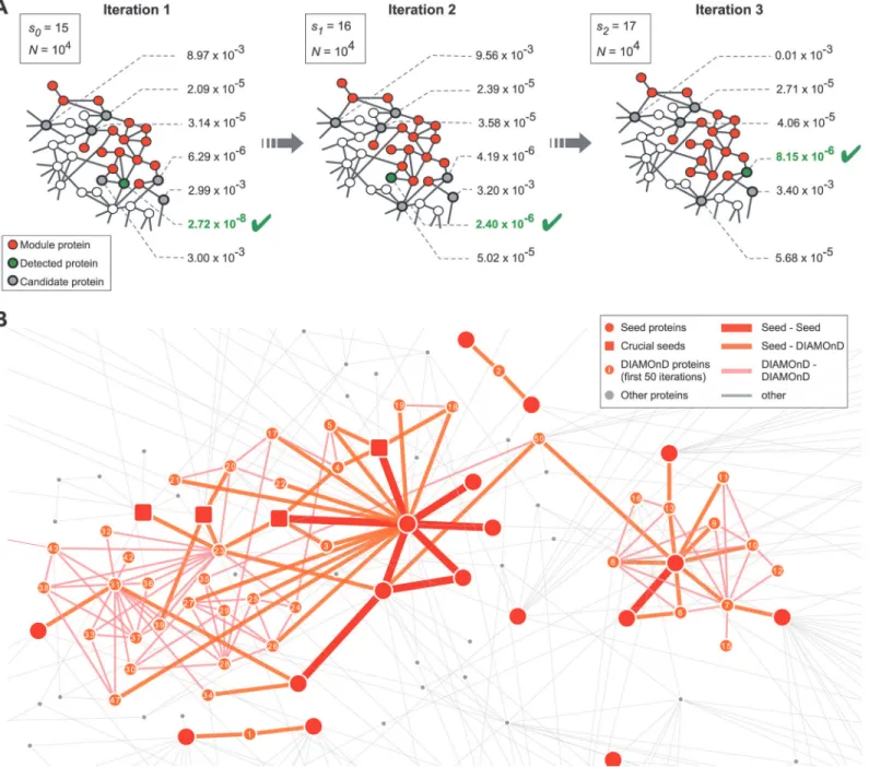
disease proteins, we propose the following algorithm to infer yetunknowndisease proteins (Fig. 2A), and hence to identify the respective disease module:
i. The connectivity significance (2) is determined for all proteins connected to any of thes0 seed proteins.
ii. The proteins are ranked according to their respectivep-values.
iii. The protein with the highest rank (i.e. lowestp-value) is added to the set of seed nodes, in-creasing their number froms0!s1=s0+1.
The procedure (i)-(iv) can be continued until the module spans across the entire network. The order in which the proteins are being pulled into the module reflects their topological rele-vance to the disease, resulting in a ranking of all proteins.Fig. 2Bshows a subgraph of the Interactome highlighting the seed proteins associated with macular degeneration and the first 50 DIAMOnD genes.
Fig 2. The DIAMOnD algorithm.(A) At each step of the iterative algorithm, theconnectivity significanceof all immediate neighbors of disease proteins is calculated. Next, the most significantly connected node (lowestp-value) is integrated into the module, thus expanding the module by one node per iteration step. (B) Subgraph of the Interactome highlighting the seed proteins formacular degenerationand the first 50 corresponding DIAMOnD proteins. In the beginning, two separate clusters grow independently until they merge at iteration step 50. Note that DIAMOnD also proposes proteins that do not have direct connections to seed proteins, e.g. at iteration steps 12 and 15. The squares mark seed proteins whose removal leads to large differences in the resulting DIAMOnD modules. The three leftmost squares, for example, enable the identification of a protein at iteration step 23, which in turn triggers the inclusion of the cluster of proteins depicted underneath, which would be absent otherwise.
Calculating tens to hundreds ofp-values at each iteration is computationally expensive; therefore we have implemented an efficient calculation to reduce the execution time (see
Materials & Methods). Furthermore, as detailed below, the algorithm can be easily adapted to incorporate additional features, in particular weighted links and/or protein associations.
Synthetic modules
In order to systematically evaluate the performance of DIAMOnD we first used a well-con-trolled test scenario by constructing synthetic modules of proteins within the Interactome. We analyzed the extent to which DIAMOnD can recover the full module if we remove the disease association from a certain fraction of proteins, thus obtaining a seed cluster that is no longer fully connected. There are many different possibilities to construct a connected set of nodes in a network, generally leading to modules with different topological properties. We implemented two different methods:
i. Shell-modules: We randomly selected one node from the network and add all its first and
second neighbors to the module (S2 Fig.A). Depending on the particular starting node, the constructed module may vary in size (S2 Fig.B). Most diseases in our curated corpus have between 50 and 150 currently identified disease proteins. Assuming that these represent only 30%-50% of all associated proteins, we chose 200 as the putative size of complete disease modules within the Interactome.
ii. Connectivity significance modules: We started from a randomly selected node and iteratively add the most significantly connected node to the module until its size reaches 200 nodes. This process produces modules with topological properties similar to those observed for real diseases.
Estimating the recovery rate
For each initially connected synthetic module, we randomly removed a certain fraction (25%, 50% and 75%) of the nodes and use the remaining nodes as seed proteins for DIAMOnD.
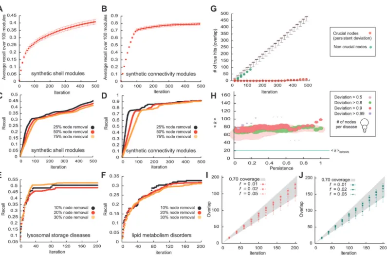
Fig. 3A and 3Bshow the fraction of recaptured initial seed nodes (recall) as a function of the number of iterations of the algorithm for 50% of the module removed. As expected, the highest rate of true positives is achieved in early iterations, so the highest ranked proteins are most like-ly to be part of the original full module.
In bothshellandconnectivitymodules, we find that the total recall of the removed nodes is relatively insensitive to the incompleteness of the seed set, i.e. the fraction of removed seed nodes (Fig. 3C,D). The observation that a similar number of proteins can be recalled from a 25% subset of the full module and from a 75% subset can be used to address a critical limitation of prioritization methods that only provide a ranking of all proteins, yet offer no objective crite-rion for the total number of biologically relevant proteins. Indeed, estimating the true positive rate is inherently difficult as the true set of proteins is by definition unknown. However, since the recall of DIAMOnD does not depend on the unknown total number of disease proteins, we can estimate it by further pruning a given incomplete set of known disease proteins. We tested this procedure on our set of 70 diseases by removing 10%, 20% and 30% of the respective known disease proteins, seeFig. 3E,Ffor two examples,blood coagulationandlipid metabolism
disorders, respectively. Generally, the recall is found to be higher when disease associations are
Analyzing the sensitivity towards perturbations
Both the network data and the disease associations are inherently noisy and expected to con-tain a considerable number of false positives. The similar recall from different levels of seed protein incompleteness suggests, however, that collectively the seed proteins and their interac-tions provide sufficient predictive power to yield robust predicinterac-tions. In order to evaluate how sensitive the DIAMOnD outcome is with respect to variations in the set of seed genes, we per-formed anN-1 analysis: We modified the initial seed protein set by removing one of thes0 pro-teins at a time, resulting ins0different DIAMOnD sets. Comparing the resulting sets of DIAMOnD proteins to the original predictions obtained from the full seed set, we find that the methodology is very robust, yielding overlaps close to 100% in most cases. Individually, most seed proteins can be removed without considerably changing the resulting DIAMOnD Fig 3. Performance evaluation of DIAMOnD.We use two different methods to construct synthetic modules (shellsandconnectivitymodules). (A, B) Recovery rate of the DIAMOnD algorithm when removing 50% of seed nodes fromshells(A) andconnectivitysynthetic modules (B), respectively. The recovery rate in synthetic modules is roughly independent of the module incompleteness. (C, D) Recovery rate when 25%, 50% and 75% of the nodes are removed fromshellsandconnectivitymodules. (E, F) Recovery rate when 10%, 20% and 30% of the nodes are removed from the disease proteins of
lysosomal storage diseasesandlipid metabolism disorders. (G) Robustness of the DIAMOnD algorithm towards small variations in the starting seed proteins (N-1 analysis). While most nodes influence the outcome very little, there are a few nodes whose removal results in a large deviation from the original outcome. This deviation may either persist across iterations (red data points) or disappear after a few iterations (green). (H) Crucial nodes are characterized by a 3–4 times higher degree. (I) DIAMOnD robustness towards random link removal from the Interactome. We identified the DIAMOnD proteins for 70 diseases in the original Interactome as well as in perturbed networks with varying fractionsfof randomly removed links. Data points and bars represent the median and median absolute deviation of the overlap (number of common proteins) between original and randomized DIAMOnD sets across 70 diseases as a function of the iteration step. (J) Same as (I), but for perturbed networks in which varying fractionsfof all links have been randomly rewired.
proteins. There are, however, typically a small number of nodes whose removal results in a drastic change of the final outcome (Figs.2Band3G). The deviation caused by a specific node removal may occur in the initial iterations and disappear over the long run (Fig. 3G, green data points) or persist across all iterations (red data points). These latter nodes are therefore more important for the integrity of the seed set.Fig. 3Hshows the degree of the nodes that cause de-viations of different persistence (seeMaterials & Methods). Crucial nodes with high persistence are characterized by a high degree (generally several fold increase compared to both average de-gree of the network,<k>= 20.7, and average degree of the disease proteins,<kdisease>= 28.9). Interestingly, we further observe that crucial nodes whose removal will be most destructive are generally not part of the largest connected component of the initial seed set. Instead, thedisease
modulesare robust towards removing disease proteins from the LCC, as these proteins will be
recovered early on due to their significant connectivity.
Similar results are obtained when noise is introduced in the underlying network (see
Materials & Methodsfor details).Fig. 3I and 3Jshow that, regardless of the method we choose to add the noisiness to the network, small variations*1% of all links in the Interac-tome have almost no effect on the obtained DIAMOnD genes. Up to 5% of the InteracInterac-tome can be completely randomized, while still retrieving more than 70% of the original set of DIAMOnD genes for more than half of all diseases.
Validating disease modules
Next we explore the performance of DIAMOnD on 70 real diseases. Since the full set of disease proteins is, by definition, unknown, we cannot assess the performance directly in terms of true positives/negatives. We therefore use publicly available gene annotation data, GeneOntology [27] and biological pathways from MSigDB [28] to validate the DIAMOnD disease modules: For each disease we determine a reference set of all significantly enriched GO-terms and pathways within the set of seed proteins. We then compare the respective annotations of each DIAMOnD gene to this reference set, assuming that proteins with annotations similar to the ones of the seed genes are more likely to be disease associated as well [1,29–32] (seeMaterials & Methodsfor details).Fig. 4A,Boffers examples for the validation according to pathway similarity for
lysosom-al storage diseases. The first*200 DIAMOnD genes are found to participate in important seed
pathways at a rate similar to the one within the seed proteins themselves and significantly higher than random expectation. In total, 58 out of 70 disease modules can be validated by either GO terms or pathways, 46 by both.Fig. 4D,Esummarizes the validation of the disease modules for all 70 diseases. The majority of the detected modules perform several times better than random expectation, in particular in the first 50–100 iterations.
Depending on the specific application, the main interest of applying DIAMOnD could lie ei-ther in selecting a small number of most promising disease protein candidates, or in obtaining a larger set of proteins to explore the molecular disease mechanisms in a broader context. For the former case, DIAMOnD directly offers a ranked list of candidates. The latter approach, however, requires an additional criterion to define the boundary of the disease module, i.e. a threshold for the total number of proteins to be considered. This threshold can be chosen by using either(i)topological or(ii)biological properties of the agglomerated proteins.
sensitively on the initial level of completeness (Fig. 3C-F). Hence, the true positive rate can be estimated by removing varying fractions of seed proteins. Forlysosomal storage disorders, for example we find an estimated recall of*50% at iteration 40 (Fig. 3E). After 40 iterations, the recall saturates and reaches a plateau, indicating that thereafter only few DIAMOnD proteins are expected to be truly disease associated. This saturation point may therefore be used as a threshold for the total number of DIAMOnD genes to consider.
(ii)A biological criterion for the threshold can be obtained from the validation according to
Fig. 4A,B. The number of DIAMOnD proteins with direct biological evidence reaches a plateau at*200 iteration steps, suggesting this as the maximal number that should be considered. A more stringent criterion is to use the significance of the enrichment (seeMaterials & Methods). The enrichment is typically strongest within the highest ranked DIAMOnD proteins and de-creases with increasing iteration steps. Forlysosomal storage diseases, for example, we find that the first 200 DIAMOnD proteins are similarly significantly enriched as the seed proteins (Fig. 4B). The largest connected component of the seed proteins aloneconsists of 24 (out of 45) proteins. When 200 DIAMOnD proteins are added, the largest connected component of the re-sulting module integrates 11 additional, previously disconnected seed proteins, rere-sulting in a module consisting of 234 proteins (Fig. 4C).Fig. 4Fshows the distribution of the fraction of in-tegrated seed proteins across 70 diseases for several iterations. We find that with increasing number of DIAMOnD genes more and more disconnected seed proteins are integrated into the module, thus allowing for an integrated analysis of their molecular mechanism.
Fig 4. Biological evaluation of DIAMOnD.(A) Validation of the DIAMOnD genes based on GeneOntology terms (seeMaterials & Methods). (B) The significance of the similarity between DIAMOnD genes and seed genes suggests a cutoff of*200 DIAMOnD genes. (C) Network representation of the lysosomal storage diseasesmodule. (D,E) Summary of the validation for all 70 disease modules based on GeneOntology (D) and biological pathways (E). (F) Fraction of seed proteins that are contained in the LCC of the DIAMOnD module for varying iteration steps. The distributions show the values obtained from 70 diseases. By introducing DIAMOnD proteins, previously disconnected seed proteins become part of the LCC.
Comparison with existing methods
In recent years, a number of disease protein prioritization methods [24,29,33–36] have been developed that can in principle be used to identify disease modules. To evaluate the relative performance of DIAMOnD, we implemented a random walk based algorithm (RW) [35] that was shown to outperform other methods and may therefore serve as a reference [29].
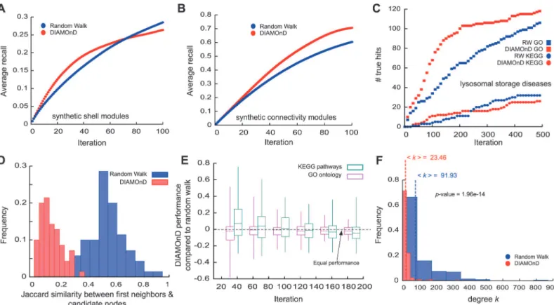
Fig. 5A,Bsummarizes the results of the comparison between DIAMOnD and RW on the synthetic modules. As we removed the attribute from half of the module nodes (about 100 nodes), iteration step 100 is a reasonable point of comparison. For both types of synthetic mod-ules we find that DIAMOnD has a higher recovery in the top 100 predictions, whereas RW captures more true hits in its late predictions. In most cases DIAMOnD is able to identify re-moved nodes in the early iterations until the recovery rate saturates (Fig. 5A). A higher initial slope corresponds to higher precision, i.e. a higher ratio of true positives TP/(TP+FP). DIA-MOnD shows higher precision and sensitivity (recall) in the initial iterations whereas RW per-forms better at later iterations once DIAMOnD saturated. In the context of disease protein identification, a high quality detection of fewer proteins with few false positives is generally more desirable than low quality detection of hundreds of proteins.
We also compared the predictions of DIAMOnD and RW for each of the 70 real disease modules, as illustrated inFig. 5Cforlysosomal storagediseases. In general, DIAMOnD offers several conceptual and practical advantages compared to previous methods: (a) Many methods Fig 5. Comparison between DIAMOnD and Random Walk (RW).(A,B) Average recovery rates of DIAMOnD and the reference RW algorithm when removing 50% (100 nodes) of 100 generatedshells(A) andconnectivity(B) modules. (C) Comparison of the biological evidence for proteins identified by DIAMOnD and RW forlysosomal storage diseases. (D) Overlap between identified proteins and immediate neighbors of seed proteins. In contrast to RW, DIAMOnD includes a considerable number of proteins without first-order interactions to seed genes. (E) Comparison of the performance of DIAMOnD and RW across 70 diseases with respect to non-specific disease data. (F) Degree distributions of the identified proteins. DIAMonD proteins are characterized by the absence of hubs.
like RW preferentially select proteins from the immediate neighborhood of the seed proteins. Surprisingly, we find that a considerable fraction of the DIAMOnD proteins do not directly in-teract with seed genes (Figs.2Band5D). DIAMOnD thereby offers disease-relevant candidates beyond first-order protein interactions. (b) Physically interacting proteins often share func-tional annotations and pathways [10,25]. As a consequence, methods like RW are expected to perform well on generic validation data. In our comprehensive analysis across 70 diseases we are limited to such generic validation data and hence observe a comparable performance when GO term similarity is used as reference. Yet, we find that when we use pathways DIAMOnD outperforms RW (Fig. 5E). Furthermore, a more focused study on a single disease that used a variety of disease-specific data, e.g. from GWAS, microarray experiments and comorbidity analysis, has experimentally confirmed the specific disease-relevance of the DIAMOnD genes and significant outperformance of DIAMOnD over RW [37]. (c) By design, DIAMOnD avoids the selection of spurious high degree nodes. Consequently, the resulting modules are generally characterized by the absence of hubs. RW proteins, in contrast, have 2–3 times higher average degree (Fig. 5F). (d) The recall rate of the DIAMOnD algorithm is roughly independent of the level of incompleteness in the seed genes. It therefore allows us to estimate the number of bio-logically relevant predictions (Fig. 3C-F). In contrast, methodologies like RW solely provide a ranking, without predicting the total number of the most probable candidates. (e) DIAMOnD shows a significantly higher recall in the early iterations compared to RW, thereby providing higher confidence candidates early on. (e) As we discuss below, the DIAMOnD algorithm can be fine-tuned for specific applications, for example by giving varying weights to the initial seed genes.
Extending the basic DIAMOnD algorithm
The DIAMOnD methodology can be easily extended to incorporate weighted links or nodes. In the iteration process introduced above, the seed proteins are treated the same way as the pre-dicted proteins agglomerated into the module at later iteration steps. We can, however, give higher weights to the seed proteins compared to those that are only predicted. This can be achieved by introducing an additional weightα>1 for the seed proteins andα= 1 for all other proteins. By considering links to nodes with higher weights to beαtimes stronger, the direct neighbors of seed proteins have a higher chance of being identified. Technically, this is imple-mented by artificially increasing the number of seed genes, for example by duplicating their number in the case ofα= 2, while maintaining their original interactions (Fig. 6A). The gener-alized form ofEquation (1)then becomes:
pðk;ks;ks0Þ ¼
sþ ða 1Þs
0
ksþ ða 1Þks0
!
N s
k ks
!
Nþ ða 1Þk
s
kþ ða 1Þk
s0
! ð3Þ
By tuningαand comparing the different resulting DIAMOnD sets we can optimize their bio-logical relevance. In synthetic modules, the recovery rate could thereby be increased 2 to 3 times in comparison to the original version of the algorithm for which the recovered fraction saturates (Fig. 6B,C). On the set of 70 diseases, the optimal values forαvary considerably (see
specific application and the validation data that are used. We also observed that introducingα allows for the construction of larger modules by helping avoid plateaus in the identification of relevant proteins (Fig. 6B-E).
Discussion
The hypothesis that disease associated proteins tend to interact with each other in the human Interactome underlies all network-based prioritization methods. Yet, for most diseases we found that only a relatively small fraction of known seed proteins in fact interact with each other. As a consequence, diseases cannot be associated with topologically dense network com-munities. Instead of the interactiondensity, we identified the interactionsignificanceas the key quantity to characterize the connection patterns among disease proteins. While in principle this could be a consequence of our currently still very limited knowledge of disease associated proteins and their interactions, our results suggest that there is in fact a fundamental difference between disease modules and topological modules. Biologically, it is indeed plausible that dis-ease modules do not necessarily coincide with densely interconnected topological modules. Highly interconnected proteins often represent functional units to perform a certain cellular task. Diseases, on the other hand, are likely to be the result of perturbations among several functional modules and therefore expected to span across functional modules/
topological communities.
Fig 6. Extending the DIAMOnD algorithm.(A) Illustration of how the algorithm can be modified to give the initial seed proteins a higher weightα= 2 by
(virtually) doubling the seed proteins while keeping their interactions. Tuningαresults in different sets of detected proteins. (B,C) Comparing the performance
for varying values ofαin synthetic shells (B) and connectivity significance (C) modules, respectively. The best results are obtained forα= 3. (C) The
performance may also saturate forαlarger than a certain value. For a given diseaseαcan be tuned to optimize the results. Performance of DIAMOnD with
respect to different values ofαis shown for ulcerative colitis (D) and nutritional and metabolic diseases (E). These plots suggest that atα= 2 the number of
true positives is maximal. (F) Overall,α*10 results in the best performance of DIAMOnD across 70 diseases. The individual values may vary considerably,
however, suggesting an individual optimization for best results.
Our analysis of the connection patterns of known disease proteins further allowed us to design a predictive and robust algorithm to uncover unknown disease associations and construct a com-prehensive disease module. For both synthetic test modules and real disease modules the recall of DIAMonD generally does not depend on the level of completeness in the initial set of seed pro-teins, but is rather a property of the module itself. This can be used to estimate the expected true positive rate in the predictions and is particularly convenient for predicting new disease associa-tions, where the total number of proteins involved in a disease is not known. While the outcome of DIAMOnD does not depend sensitively on the exact set of seed proteins, there typically are a few crucial seed proteins whose omission leads to drastically different and presumably random results. These crucial proteins are characterized by their high degree. Their topological impor-tance suggests also particularly important roles for the pathobiological mechanisms of the disease. Overall, the final disease modules typically consist of one large component that contains all DIA-MOnD genes and 30%-60% of the initially disconnected seed proteins, the rest remaining discon-nected. The integration of the several initially disconnected seed clusters into a broader disease module and the elucidation of the network paths that interconnect them is crucial for a holistic understanding of the pathobiology and molecular mechanisms underlying complex diseases. Whether the remaining disconnected seed proteins could be integrated if the Interactome data was more complete, or whether their disease associations are spurious remains an open question.
Materials and Methods
Interactome construction
We only consider direct physical protein interactions with reported experimental evidence. For this, we consolidated several data sources as described in [12]:
i. Regulatory interactions: We used the TRANSFAC [38] database that lists regulatory interac-tions derived from the presence of a transcription factor binding site in the promoter region of a certain gene. The resulting network consists of 774 transcription factors and genes con-nected via 1,335 interactions.
ii. Binary interactions: We combine several yeast-two-hybrid high-throughput datasets [10,39–42] with binary interactions from IntAct [43] and MINT [44] databases. The sum of these data sources yields 28,653 interactions between 8,120 proteins.
iii. Literature curated interactions: These interactions, typically obtained by low throughput experiments, are manually curated from the literature. We use IntAct, MINT, BioGRID [45] and HPRD [46], resulting in 88,349 interactions between 11,798 proteins.
iv. Metabolic enzyme-coupled interactions: Two enzymes are assumed to be coupled if they share adjacent reactions in the KEGG and BIGG databases. In total, we use 5,325 such met-abolic links between 921 enzymes from [47].
v. Protein complexes: Protein complexes are single molecular units that integrate multiple gene products. The CORUM database [48] is a collection of mammalian complexes derived from a variety of experimental tools, from co-immunoprecipitation to co-sedimentation and ion exchange chromatography. In total, CORUM yields 2,837 complexes with 2,069 proteins connected by 31,276 links.
vii. Signaling interactions: The dataset from [50] provides 32,706 interactions between 6,339 proteins that integrate several sources, both high-throughput and literature curation, into a directed network in which cellular signals are transmitted by proteins-protein interac-tions. Note that we do not take the direction of these interactions into account.
The union of all interactions from(i)-(vii)yields a network of 13,460 proteins that are inter-connected by 141,296 physical interactions.
Disease-gene associations
The corpus of 70 diseases was manually chosen by a medical expert, with the additional criteria of at least 20 associated genes reported in the literature. The gene-disease associations were re-trieved from OMIM (Online Mendelian Inheritance in Man;http://www.ncbi.nlm.nih.gov/ omim) [51] and GWAS (Genome-Wide Association Studies. The OMIM associations we use also include associations from UniProtKB/Swiss-Prot and have been compiled by [13]. The disease-gene associations from GWAS are obtained from the PheGenI database (Phenotype-Genotype Integrator;http://www.ncbi.nlm.nih.gov/gap/PheGenI) [9] that integrates various NCBI genomic databases. We use a genome-wide significance cutoff ofp-value510–8.
Local modularity
R
To quantify the extent to which disease proteins correspond to topological communities, we use thelocal modularity R[23]. The community character of a set of nodesCis determined by the“sharpness”of its boundary, i.e by how well it is separated from the rest of the network. The boundaryBconsists of all nodes inCthat have connections to nodes outside the commu-nity (Fig. 1K). The local modularityRis then defined as the number of links attached to nodes inBthat do not leave the community, normalized by their total number of links. This can be written as
R¼
X
ij
Bijdði;jÞ
X
ij
Bij
whereBijis the adjacency matrix of the boundary nodes andδ(i,j) = 1 if both nodesiandjare inC, otherwiseδ(i,j) = 0.
The comparison with random control was done by selecting for each disease the same num-ber of proteins at random from the Interactome (100 times). We then used a Kolmogorov-Smirnoff test to estimate the significance of the difference between the distribution of disease proteins and the respective distribution obtained in the randomization.
Topological community detection methods
We use three well-established, methodologically distinct algorithms:
i. A link community algorithm from [14], which provides a hierarchical clustering of all links in the network. We use the default cut-off at the optimal partition density.
ii. The parameter-free Louvain method [21], which maximizes the global modularity of the network.
Random walk based disease gene prioritization
We implemented a method from [35] that prioritizes candidate genes based on network diffu-sion. The seed genes serve as starting points for a random walker that wanders from node to node along the links of the network. At every time step of the iterative algorithm, the walker moves to a randomly selected neighbor of its current position. After every move the walker is reset to a randomly chosen seed gene with a given probabilityr(we user= 0.4). After a suffi-cient number of iterations the frequency with which the nodes in the network are visited con-verges and can be used to rank the corresponding genes. Genes that are visited more often are considered to be closer to the seed genes and therefore more relevant to the disease than those who are visited less often.
Network randomization
We use two models to construct ensembles of randomized networks with varying degrees of noise and incompleteness compared to the original Interactome:
i. To investigate the effects of network incompleteness we constructpruned networksby re-moving a fraction of randomly selected links from the Interactome.
ii. To explore the impact of noise in the Interactome we usepartially rewired networksin which a fraction of randomly selected links are split and then randomly reconnected. This procedure corresponds to the configuration model [52,53] and does not alter the degrees of the nodes, i.e. only the specific interaction partners of the nodes are randomized, not their overall number. Note that the original network is perturbed considerably even at small frac-tions of rewired links as both existing links are removed and simultaneously new ones are established.
DIAMOnD implementation
The number of times we need to calculate the computationally relatively expensivep-values can be considerably reduced by noticing that two proteins with the same values of eitherksork can be ranked directly according to their value in the respective other parameter, see Eqs.(1)
and(2): If two proteins have the same degreek, the one with higherkswill result in less terms in the sum inEq. (2)and consequently a lowerp-value. Similarly, between two proteins with the same number of connections to seedsks, the one with lowerkwill result in lowerp-value. This results in the following procedure: At each iteration step, we first classify the nodes based on their ksand rank the node with lowestkhighest within that class. Next, we classify the top ranks of each class by their degreekand choose the ones with highestks.Finally, we calculate the exactp-value for the remaining nodes. This procedure guarantees that the number of can-didate nodes will reduce to at mostsnodes per iteration, askscannot exceeds(note thatsi!
si+1 at each iteration). In the worst-case scenario, and without further reducing the candidate nodes by their degreek, we are left withsnodes for which we need to calculatep-values. As-suming we need to identifyNnodes from the network, the time complexity of the algorithm is of the orders+(s+1)+. . .+(N-1)+N*NðN 1Þ
2 =O(N
2). This compares favorably with other well
established algorithms such as the random walk based method, whose complexity is betweenO
(NlogN) andO(N3) [54,55].
Topological validation,
N-1
analysis and persistence
many iterations:
deviation¼1 overlap
where theoverlapis measured by the number of proteins that are in common between the orig-inal DIAMOnD outcome and the DIAMOnD outcome after the removal of seed genes. The
persistenceof a deviation is measured as
Persistence¼Total number of iteration steps where the deviation persists Total number of iterations
High persistence indicates that the removal of a node results in a deviation that holds across all iterations. However, typically we find that the perturbations introduced by removing a sin-gle seed node are compensated after a few iterations.
Gene annotations
We use Gene Ontology (GO) for all genes are extracted from [http://www.geneontology.org/, downloaded Nov. 2011]. We only use high confidence annotations associated with the evidence codes EXP, IDA, IMP, IGI, IEP, ISS, ISA, ISM or ISO. In particular, we do not use annotations inferred from physical interactions (evidence code IPI) in order to avoid circularity. To obtain a complete set of GO terms from the reported most specific term for each gene, all annotations are propagated upwards on the full tree.
The pathway annotations are extracted from the Molecular Signatures Database (MSigDB) published by the Broad Institute, Version 3.1 [56]. MSigDB integrates several different pathway databases; we use the ones from KEGG, Biocarta and Reactome.
Biological validation analysis
To validate the potential disease relevance of the predicted candidate genes (from either DIA-MOnD or RW), we compare their biological characteristics to the ones of the initial seed genes using the following workflow:
i. First we identify the set of GO terms (pathways) that are significantly enriched within the given set of seed genes using Fisher’s exact test (Bonferroni correctedp-value<0.5).
ii. For each candidate gene we then check whether it is annotated with any of these significant terms. Genes with common annotations are considered as true positives.
Supporting Information
S1 Fig. Size distribution of the topological communities in the Interactome as identified by (A) link clustering, (B) the Louvin method and (C) the MCL method.(D-F) Number of com-munity-disease pairs with significant overlap vs. theirJaccardsimilarityJfor the three meth-ods. No identified topological community coincides (J= 1) with a full set of disease genes. (EPS)
S2 Fig. Properties of the syntheticShellmodules.(A) Illustration of the construction process:
An initial node is selected at random and all first and second neighbors are added to the mod-ule. The exact topological properties of the resulting modules depend on the initial node. Panel (B) shows how the synthetic module size varies with the degree of the initial node.
(EPS)
S1 Data. Annotated Interactome data. (TSV)
S2 Data. Disease gene association data for 70 diseases. (TSV)
S1 Code. A python implementation of the DIAMOnD algorithm. (PY)
Acknowledgments
The authors would like to thank J. Loscalzo for expert selection of phenotypes, A. Sharma, J. Bagrow, E. Guney, A. Karma, D. Chasman, R. Movassaghi Jorshari, M. Saltolini, M. Kitsak and S. Rabello for helpful discussions, and suggestions and J. De Nicolo for website design.
Author Contributions
Conceived and designed the experiments: SDG JM ALB. Performed the experiments: SDG. An-alyzed the data: SDG JM. Contributed reagents/materials/analysis tools: SDG JM. Wrote the paper: SDG JM ALB.
References
1. Goh KI, Cusick ME, Valle D, Childs B, Vidal M, et al. (2007) The human disease network. Proceedings of the National Academy of Sciences of the United States of America 104: 8685–8690. PMID:
17502601
2. Pawson T, Linding R (2008) Network medicine. FEBS letters 582: 1266–1270. doi:10.1016/j.febslet. 2008.02.011PMID:18282479
3. Schadt EE (2009) Molecular networks as sensors and drivers of common human diseases. Nature 461: 218–223. doi:10.1038/nature08454PMID:19741703
4. Zanzoni A, Soler-Lopez M, Aloy P (2009) A network medicine approach to human disease. FEBS let-ters 583: 1759–1765. doi:10.1016/j.febslet.2009.03.001PMID:19269289
5. Barabasi AL, Gulbahce N, Loscalzo J (2011) Network medicine: a network-based approach to human disease. Nature reviews Genetics 12: 56–68. doi:10.1038/nrg2918PMID:21164525
6. Buchanan M, Caldarelli GDLR, P (2010) Networks in cell biology: Cambrdige University Press. 7. Feldman I, Rzhetsky A, Vitkup D (2008) Network properties of genes harboring inherited disease
muta-tions. Proceedings of the National Academy of Sciences of the United States of America 105: 4323– 4328. doi:10.1073/pnas.0701722105PMID:18326631
8. del Sol A, Balling R, Hood L, Galas D (2010) Diseases as network perturbations. Current opinion in bio-technology 21: 566–571. doi:10.1016/j.copbio.2010.07.010PMID:20709523
resources. European journal of human genetics: EJHG 22: 144–147. doi:10.1038/ejhg.2013.96PMID:
23695286
10. Venkatesan K, Rual JF, Vazquez A, Stelzl U, Lemmens I, et al. (2009) An empirical framework for bina-ry interactome mapping. Nature methods 6: 83–90. doi:10.1038/nmeth.1280PMID:19060904
11. Driel HGBaMAv (2004) From syndrome families to functional genomics. Nature Reviews Genetics 5. 12. Menche J, Sharma A, Kitsak M, Ghiassian S, Vidal M, et al. (2015) Uncovering disease-disease rela-tionships through the incomplete human interactome. Science 347, no. 6224: 1257601 doi:10.1126/ science.1257601PMID:25700523
13. Mottaz A, Yip YL, Ruch P, Veuthey AL (2008) Mapping proteins to disease terminologies: from UniProt to MeSH. BMC bioinformatics 9 Suppl 5: S3. doi:10.1186/1471-2105-9-S5-S3PMID:18460185
14. Ahn YY, Bagrow JP, Lehmann S (2010) Link communities reveal multiscale complexity in networks. Nature 466: 761–764. doi:10.1038/nature09182PMID:20562860
15. Clauset A, Newman M, Moore C (2004) Finding community structure in very large networks. Physical Review E 70.
16. Fortunato S (2010) Community detection in graphs. Physics Reports 486: 75–174.
17. Girvan M, Newman ME (2002) Community structure in social and biological networks. Proceedings of the National Academy of Sciences of the United States of America 99: 7821–7826. PMID:12060727
18. Lancichinetti A, Fortunato S (2009) Community detection algorithms: A comparative analysis. Physical Review E 80.
19. Newman M (2004) Fast algorithm for detecting community structure in networks. Physical Review E 69.
20. Newman M, Girvan M (2004) Finding and evaluating community structure in networks. Physical Review E 69.
21. Blondel VD, Guillaume J-L, Lambiotte R, Lefebvre E (2008) Fast unfolding of communities in large net-works. Journal of Statistical Mechanics: Theory and Experiment 2008: P10008. PMID:19002269
22. Bagrow J, Bollt E (2005) Local method for detecting communities. Physical Review E 72. 23. Clauset A (2005) Finding local community structure in networks. Physical Review E 72.
24. Van Dongen S (2008) Graph Clustering Via a Discrete Uncoupling Process. SIAM Journal on Matrix Analysis and Applications 30: 121–141.
25. Sharan R, Ulitsky I, Shamir R (2007) Network-based prediction of protein function. Molecular systems biology 3: 88. PMID:17353930
26. Hart GT, Ramani AK, Marcotte EM (2006) How complete are current yeast and human protein-interac-tion networks? Genome biology 7: 120. PMID:17147767
27. Ashburner M, Ball CA, Blake JA, Botstein D, Butler H, et al. (2000) Gene Ontology: tool for the unifica-tion of biology. Nature Genetics 25: 25–29. PMID:10802651
28. Kanehisa M, Goto S, Kawashima S, Okuno Y, Hattori M (2004) The KEGG resource for deciphering the genome. Nucleic acids research 32: D277–280. PMID:14681412
29. Navlakha S, Kingsford C (2010) The power of protein interaction networks for associating genes with diseases. Bioinformatics 26: 1057–1063. doi:10.1093/bioinformatics/btq076PMID:20185403
30. Su AI, Wiltshire T, Batalov S, Lapp H, Ching KA, et al. (2004) A gene atlas of the mouse and human pro-tein-encoding transcriptomes. Proceedings of the National Academy of Sciences of the United States of America 101: 6062–6067. PMID:15075390
31. B. GTK, J. Z, S. M, L. K, N. CK (2006) Analysis of the human protein interactome and comparision with yeast, worm and fly interaction datasets. doi:10.1038/1747.
32. Xu J, Li Y (2006) Discovering disease-genes by topological features in human protein-protein interac-tion network. Bioinformatics 22: 2800–2805. PMID:16954137
33. Oti M, Snel B, Huynen MA, Brunner HG (2006) Predicting disease genes using protein-protein interac-tions. Journal of medical genetics 43: 691–698. PMID:16611749
34. Lage K, Mollgard K, Greenway S, Wakimoto H, Gorham JM, et al. (2010) Dissecting spatio-temporal protein networks driving human heart development and related disorders. Molecular systems biology 6: 381. doi:10.1038/msb.2010.36PMID:20571530
35. Kohler S, Bauer S, Horn D, Robinson PN (2008) Walking the interactome for prioritization of candidate disease genes. American journal of human genetics 82: 949–958. doi:10.1016/j.ajhg.2008.02.013
PMID:18371930
37. Sharma A, Menche J, Huang C, Ort T, Zhou X, et al. (2015) A disease module in the interactome ex-plains disease heterogeneity, drug response and captures novel pathways and genes for Asthma. Hum. Mol. Genet. first published online January 12, 2015, doi:10.1093/hmg/ddv001.
38. Matys V (2003) TRANSFAC(R): transcriptional regulation, from patterns to profiles. Nucleic acids re-search 31: 374–378. PMID:12520026
39. Rual JF, Venkatesan K, Hao T, Hirozane-Kishikawa T, Dricot A, et al. (2005) Towards a proteome-scale map of the human protein-protein interaction network. Nature 437: 1173–1178. PMID:16189514
40. Stelzl U, Worm U, Lalowski M, Haenig C, Brembeck FH, et al. (2005) A human protein-protein interac-tion network: a resource for annotating the proteome. Cell 122: 957–968. PMID:16169070
41. Yu H, Tardivo L, Tam S, Weiner E, Gebreab F, et al. (2011) Next-generation sequencing to generate interactome datasets. Nature methods 8: 478–480. doi:10.1038/nmeth.1597PMID:21516116
42. Rolland T, Ta An M, Charloteaux B, Pevzner SJ, Zhong Q, et al. (2014) A proteome-scale map of the human interactome network. Cell 159: 1212–1226. doi:10.1016/j.cell.2014.10.050PMID:25416956
43. Aranda B, Achuthan P, Alam-Faruque Y, Armean I, Bridge A, et al. (2010) The IntAct molecular interac-tion database in 2010. Nucleic acids research 38: D525–531. doi:10.1093/nar/gkp878PMID:
19850723
44. Ceol A, Chatr Aryamontri A, Licata L, Peluso D, Briganti L, et al. (2010) MINT, the molecular interaction database: 2009 update. Nucleic acids research 38: D532–539. doi:10.1093/nar/gkp983PMID:
19897547
45. Stark C, Breitkreutz BJ, Chatr-Aryamontri A, Boucher L, Oughtred R, et al. (2011) The BioGRID Interac-tion Database: 2011 update. Nucleic acids research 39: D698–704. doi:10.1093/nar/gkq1116PMID:
21071413
46. Keshava Prasad TS, Goel R, Kandasamy K, Keerthikumar S, Kumar S, et al. (2009) Human Protein Reference Database—2009 update. Nucleic acids research 37: D767–772. doi:10.1093/nar/gkn892
PMID:18988627
47. Lee DS, Park J, Kay KA, Christakis NA, Oltvai ZN, et al. (2008) The implications of human metabolic network topology for disease comorbidity. Proceedings of the National Academy of Sciences of the United States of America 105: 9880–9885. doi:10.1073/pnas.0802208105PMID:18599447
48. Ruepp A, Waegele B, Lechner M, Brauner B, Dunger-Kaltenbach I, et al. (2010) CORUM: the compre-hensive resource of mammalian protein complexes—2009. Nucleic acids research 38: D497–501. doi:
10.1093/nar/gkp914PMID:19884131
49. Hornbeck PV, Kornhauser JM, Tkachev S, Zhang B, Skrzypek E, et al. (2012) PhosphoSitePlus: a comprehensive resource for investigating the structure and function of experimentally determined post-translational modifications in man and mouse. Nucleic acids research 40: D261–270. doi:10.1093/nar/ gkr1122PMID:22135298
50. Vinayagam A, Stelzl U, Foulle R, Plassmann S, Zenkner M, et al. (2011) A directed protein interaction network for investigating intracellular signal transduction. Science signaling 4: rs8. doi:10.1126/ scisignal.2001699PMID:21900206
51. Hamosh Ada AFS, Amerger Joanna, Bocchini Carol, Valle David and McKusick Victor A. (2002) a knowledgebase of human genes and genetic disorders. Nucleic Acids Researcg 30.
52. Newman MEJ (2003) The Structure and Function of Complex Networks; REVIEW S, editor. 53. Canfield EABaER (1978) The asymptotic number of labeled graphs with given degree sequences.
Combinatorial Theory 24: 296–307.
54. Feige U (1995) A tight lower bound on the cover time for random walks on graphs. Random Structures and Algorithms pp. 433–438.
55. Feige U (1995) A tight upper bound on the cover time for random walks on graphs. Random Structures and Algorithms pp. 51–54.
56. Subramanian A, Tamayo P, Mootha VK, Mukherjee S, Ebert BL, et al. (2005) Gene set enrichment analysis: a knowledge-based approach for interpreting genome-wide expression profiles. Proceedings of the National Academy of Sciences of the United States of America 102: 15545–15550. PMID: