Bertrand Equilibria and Sharing Rules
Steffen H. Hoernig
∗School of Economics, Universidade Nova de Lisboa
Campus de Campolide, 1099-032 Lisboa, Portugal
CEPR, London
March 2005
JEL: C72, D43, L13
∗[email protected], tel. +351-213801645, fax +351-213870933. I would like to thank
Fernando Branco for helpful discussions, the audience at Pompeu Fabra (Barcelona), ISEG (Lisbon), University of Mannheim, ESEM 2003 (Venice), two anonymous referees, and the editor Dan Kovenock for useful comments. This research received financial support under project POCTI/ECO/37925/2001 of FCT and FEDER.
Abstract
We analyze how sharing rules affect Nash equilibria in Bertrand games, where the sharing of profits at ties is a decisive assumption. Necessary con-ditions for either positive or zero equilibrium profits are derived. Zero profit equilibria are shown to exist under weak conditions if the sharing rule is “sign-preserving”. For Bertrand markets we define the class of “expectation sharing rules”, where profits at ties are derived from some distribution of quantities. In this class the winner-take-all sharing rule is the only one that is always sign-preserving, while for each pair of demand and cost functions there may be many others.
JEL: C72, D43, L13
Keywords: Bertrand games, Sharing rule, Tie-breaking rule, Sign-preserving sharing rules, Expectation sharing rules
1
Introduction
Existence and multiplicity of pure and mixed strategy Nash equilibria in Bertrand pricing games have been widely researched. The results obtained depend on properties of the demand and production cost specifications, and on the sharing or tie-breaking rule embodied in the payoffs. While the former have been the subject of some investigation, the latter went almost unnoticed. This is surprising because the sharing rule has a decisive role to play because candidate equilibria will often involve ties at the lowest price.
The contribution of our research is two-fold. First, we consider “Bertrand games” with generic payoffs, not necessarily derived from some demand and cost function. Second, we put the sharing rule into the foreground. No a priori restrictions are imposed on their shape; rather, we discover which properties that have an effect on equilibria.
In doing so, we find necessary conditions on a single player’s payoff on the one hand, and on the sharing rules on the other hand, for the emergence of positive or zero equilibrium payoffs for some or all players. The only relevant condition on sharing rules in this context is that they be “tie-decreasing”, that is, a tied firm’s payoffs should be below a single firm’s at the same price. These results are then used to state a general result about the necessity of zero equilibrium profits.
We also demonstrate how to prove quickly whether a given Bertrand game has neither pure nor mixed strategy Nash equilibria. In zero-sum games this is not very difficult: It is enough to prove that the maximin and minmax value differ, see [13]. For non-zero-sum games like Bertrand competition with variable demand, however, this is a surprisingly hard exercise.
class of sharing rules, zero-profit Nash equilibria exist if a single firm’s pay-offs are continuous. Therefore under sign-preserving sharing the classical “Bertrand paradox” of zero profits is restored, with the new interpretation that “price is equal to average cost”. The “competitive outcome” of price equal to marginal cost turns out to be the exception rather than the rule, and generically occurs only under constant returns to scale. These results therefore shed new light on the question of “Bertrand paradox” outcomes of zero equilibrium profits, generalizing [8] and [3] to arbitrary payoffs and sharing rules.
Finally, for Bertrand pricing games we define the class of “expectation sharing rules”, where a tied firm’s payoff is defined as the expectation over some distribution of quantities. We concentrate on the case where the total quantity allocated to firms is equal to quantity demand by consumers. Two known sharing rules are part of this class: The classical sharing rule is “equal sharing”, where each firm receives an identical share with certainty. For the case where each firm is equally like to receive all demand, [3] have introduced the notion of “winner-take-all” sharing, but this sharing rule appeared at least in [11] and [2], and is referred to in [14, p. 139]. We show that there are pairs of demand and cost functions for which either all or at least an infinite number of expectation sharing rules are sign-preserving. On the other hand, only the winner-take-all sharing rule is sign-preserving under all circumstances.
The literature on the Bertrand model at first concentrated on constant returns to scale. For two firms and equal sharing, [6] has shown that pricing at marginal cost is the unique equilibrium when demand is bounded, con-tinuous and has a finite choke-off price. With more than two firms there is a continuum of zero-payoff equilibria where at least two firms always choose
price equal to marginal cost, and the other firms randomize arbitrarily be-tween prices not lower than marginal cost. This multiplicity of equilibria is “inessential” in the sense that equilibrium production, profits and consumer welfare are the same for all these equilibria.
On the other hand, [8] have shown that infinite monopoly payoffs are not only sufficient but also necessary in duopoly for Nash equilibria other than the zero-payoff equilibrium to obtain. In the context of winner-take-all sharing, [2] have also demonstrated the existence of these equilibria, but not shown necessity of infinite monopoly payoffs.
If returns to scale in the Bertrand model are not constant then the sit-uation is much more complicated. [5] showed that under decreasing returns to scale there is a continuum of pure strategy equilibria where firms make positive profits. Later, [7] amplified this result by proving that in this case there are continua of mixed equilibria on finite and continuous supports. On the other hand, below we present an example where under increasing returns to scale neither pure nor mixed strategy Nash equilibria exist.
An alternative approach where sharing rules are part of the equilibrium, rather than part of the definition of the game, is that of “games with endoge-nous sharing rules” of [12]. Recently, [1] has shown that endogeendoge-nous sharing rules can be constructed from continuous (instead of discrete) approxima-tions to payoffs, which paves the way to finding them analytically. In this context a sharing rule is some selection from the convexification of payoffs at discontinuities. While there is always a selection such that an equilibrium exists, nothing can be said a priori about the shape of this selection, which may be highly sensitive to the specification of the model.
In Section 2 we set out the model and define sharing rules. Nash equilibria are analysed in Section3. Section4 deals with sign-preserving sharing, while
Section 5 analyses expectation sharing rules. Section 6 concludes. Almost all proves are in the Appendix.
2
The Model
Let N = {1, .., n} be a set of n identical players who simultaneously chooses actions p ∈ R+. Denote by T (p1, .., pn) = {j ∈ N|pj = min{p1, .., pn}} the
set of “winners”, i.e. players tied at the smallest action, and let πm(p)denote
the payoffs of the m = |T (pi, p−i)| ∈ N winners at action p. Players who are
not winners receive zero payoffs. With p−i = (p1, .., pi−1, pi+1, .., pn), player
i’s payoff is then given by
u (pi, p−i) = ⎧ ⎨ ⎩ π|T (pi,p−i)|(pi) if i∈ T (pi, p−i) 0 if i /∈ T (pi, p−i) . (1)
Let M = {2, .., n}. Typically π1 is defined by the fundamentals of the game,
while the {πm}m∈M define the sharing rule, incorporating additional
assump-tions.
The above definition of payoffs can be extended to mixed strategies, that is, cumulative distribution functions, as in [9]. Let ∆ be the set of mixed strategies on R+. If Fj ∈ ∆, j 6= i, F−i = (F1, .., Fi−1, Fi+1, .., Fn) and
Ni = N\ {i}, then u (pi, F−i) = X T ⊂Ni π|T |+1(pi) Ã Y j∈T αj(pi) ! ⎛ ⎝ Y k∈Ni\T (1− Fk(pi)) ⎞ ⎠ , (2) where αj(p) = Fj(p)− limp0%pFj(p0) is the size of the atom (if any) in
Fj at p ∈ R+. The summation is over the sets T of players that may be
tied with player i at action pi. For any N0 ⊂ N and action p ∈ R+ let
an atom at p. The games that we will consider are “Bertrand games” Γ =
N, ∆, π1,{πm}m∈M
® .
In the Bertrand model players are firms in an industry selling a homo-geneous good, and actions are prices. If D, C : R+ → R+ are a the
de-mand and cost functions, respectively, a single firm’s payoffs are π1(p) =
pD (p)− C (D (p)).
More generally, this setup includes all static games of complete informa-tion where players are symmetric, strategy spaces are completely ordered, the winners’ payoff only depends on the winning action and the number of winners, and any player who plays a higher action receives zero payoffs. This set includes some first-price auctions (after inverting the strategy spaces).
As we defined them, sharing rules are mappings (p, m) 7→ πm(p). For
most of the analysis we need not specify this mapping further, but in Section 5 we consider the specific class of expectation sharing rules. By way of com-parison, the definition of an endogenous sharing rule of [12] in the specific context of the Bertrand model, roughly, amounts to some arbitrary selection from the convexification of π1 at its discontinuities. This cannot reproduce
the payoffs all Bertrand models with decreasing returns to scale, since payoffs πm at ties may lie outside the convex hull of π1.
Two well-known sharing rules in the Bertrand model are equal sharing and winner-take-all sharing. Equal sharing amounts to πm(p) = pD (p) /m−
C (D (p) /m): Each firm receives an equal share of demand. This is the shar-ing rule traditionally posited. Winner-take-all sharshar-ing W implies that one randomly selected firm receives all demand, and results in expected profits πm(p) = π1(p) /m. This latter sharing rule has appeared in [11], [2] and [3].
c≥ 0, the payoffs under the two sharing rules coincide,
πm(p) = pD (p) /m− cD (p) /m = π1(p) /m (3)
This equivalence of payoffs under constant returns to scale in the Bertrand model may explain why the subject of sharing rules as such has not yet re-ceived much attention. Generally payoffs between these two sharing rules differ, with drastic consequences. If winner-take-all sharing is assumed, exis-tence and uniqueness of symmetric pure strategy equilibria are almost trivial, as shown below. Under equal sharing the situation is much more complicated, with the possible outcomes of non-existence of equilibrium or existence of a continuum of equilibria depending on the returns to scale.
Many reasonable conditions can be imposed on sharing rules. For now we restrict the class of allowable sharing rules as little as possible. Let us first make the following definitions:
Definition 1 A function f : R → R is
1. zero-at-zero (ZAZ) if f (x) = 0 if x = 0;
2. sign-preserving (SP) if f (x)T 0 if and only if x T 0 for all x ∈ R. A sign-preserving function is necessarily zero-at-zero. Two classes of shar-ing rules of special interest are:
Definition 2 Given π1, a sharing rule {πm}m∈M
1. is sign-preserving if πm(p) has the same sign as π1(p), for all m∈ M
and p ∈ R+;
2. is tie-decreasing at a price p ∈ R+ if π1(p) > maxm∈Mπm(p) whenever
It follows immediately from this definition that for any strictly increasing and zero-at-zero function z ∈ R → R the sharing rule {z (πm)}m∈M is SP
if {πm}m∈M SP. While equal sharing is not SP if returns to scale are not
constant, winner-take-all sharing is SP for all π1. Therefore any z (W ) is also
SP, and there always exist infinitely many SP sharing rules for all payoffs π1.
A sharing rule is tie-decreasing if payoffs at ties are below a single player’s payoff at the same price. The role of tie-decreasing sharing rules emerges when we consider Nash equilibria with positive profits in the next section. Winner-take-all sharing is tie-decreasing, while equal sharing is not under decreasing returns to scale.
3
Nash Equilibria and Sharing Rules
In this section we will derive general characteristics of Bertrand equilibria, i.e. the Nash equilibria of Bertrand games. We describe whether and how these are related to properties of the sharing rule or of the demand and cost functions. Starting from the assumption that equilibria exist, there is surprisingly much that one can say without presupposing a given sharing rule. We first analyze equilibria involving positive expected profits for some firms, and then state a general theorem that describes when all Bertrand equilibria must involve zero profits.
Let (F∗
1, .., Fn∗) ∈ Sn be a Nash equilibrium, with equilibrium payoffs
Πi = ui ¡ Fi∗, F−i∗ ¢ : ui ¡ Fi∗, F−i∗ ¢≥ ui ¡ Fi, F−i∗ ¢ ∀ Fi ∈ S, ∀ i ∈ {1, .., n} . (4)
For all i ∈ N let Si be the support of firm i’s equilibrium strategy Fi, then
Si is closed and bounded from below. Necessarily ui
¡ pi, F−i∗
¢
pi ∈ R+, and ui
¡ pi, F−i∗
¢
= Πi for all pi ∈ Pi = Si\Zi, where Zi is a set of Fi∗
-measure zero such that ui
¡ pi, F−i∗
¢
< Πi for all pi ∈ Zi. The fact there may
be prices pi ∈ Si with ui
¡ pi, F−i∗
¢
< Πi complicates some of our arguments
below.
We first highlight some of the complexities that can be encountered when the assumption of constant returns to scale is abandoned.
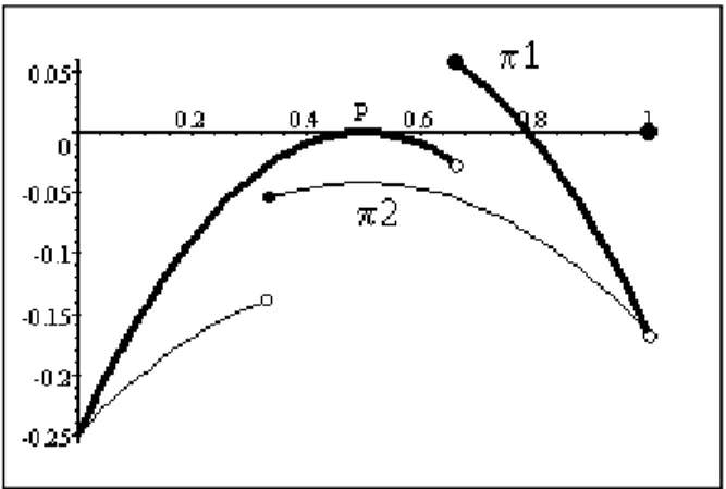
Example: In a market with two symmetric firms demand is D (p) = max{0, 1 − p}, and the cost function is given by c (0) = 0, c (q) = 1/6 for q ∈ (0, 1/3], and c (q) = 1/4 for q > 1/3. With equal sharing there is no symmetric pure strategy equilibrium, but a pair of asymmetric pure strategy equilibria with pi = 2/3 (at the left-discontinuity) and pj = 1/2, with both
firms i, j making zero profits. Furthermore, there is a continuum of mixed strategy equilibria where firm i plays pi = 2/3 with certainty, while firm
j randomizes between an atom at pj = 1/2 and prices larger than 2/3.
Expected payoffs in this case are Πi = (1− α∗2(1/2)) /18, and Πj = 0. With
winner-take-all sharing, there are two symmetric pure strategy equilibria: p = 1/2 (zero profits), and p = 2/3 (positive profits), and a continuum of asymmetric ones with pi = 1/2and pj ∈ (1/2, 2/3) (zero profits).
<< HERE FIGURE 1 >>
This example shows that one may find equilibria where some firms make positive profits while others make zero profits. This happens even though firms are ex ante symmetric. Furthermore, there may be many such equilib-ria. We have found equilibria where the firm making zero equilibrium profits sometimes plays lower prices than the firm making positive profits, demon-strating that the “intuition” that only firms charging the lowest price have a chance of making any profit is wrong.
[5] has shown that there under equal sharing and decreasing returns to scale there may be a continuum of symmetric equilibria involving positive profits. Furthermore, [7] demonstrates that in this case there also are in-finitely many mixed equilibria where firms gain positive expected profits and the sets Pi are continua. All of this is shown in a context of finite monopoly
profits, so that the “bootstrap” results of [2] and [8] do not apply.
Let J>={i ∈ N | Πi > 0} and J= ={i ∈ N | Πi = 0} be the sets of firms
with positive and zero expected equilibrium profits, respectively. There can be none with negative profits, given that C (0) = 0 and deviations to higher prices are always possible. The following lemma lists some of the properties of Bertrand equilibria where some firms have positive profits. These results are independent of the sharing rule. Let “maximum profits” be defined as πmax = sup
p∈R+,k∈Nπk(p). In the classic Bertrand model with ES and
con-stant marginal costs these are equal to monopoly profits suppπ1(p).
Lemma 1 Given a Bertrand Γ, assume that πmax<
∞ and that (F∗
1, .., Fn∗)
is a Nash equilibrium with J> 6= ∅. Then:
1. There is a price t ∈ R+ such that t = max Si for all i ∈ J>. If
|J>| > 1 then Fj∗(t) < 1 for all j ∈ J=, and there exists K ∈ R+
such that α∗
i (t) Πi = K for all i ∈ J>. If J> = {k} and J= 6= ∅, then
Fj∗(t) < 1 + α∗j(t) for all j ∈ J=, and α∗k(t) > 0 or there is a sequence
{pl}∞l=1 ⊂ Sk such that α∗k(pl) > 0 for all l and liml→∞pl = t.
2. Let J= 6= ∅. For all firms i ∈ J> the sets Pi are countable, and
P
p∈Piα
∗
i (p) = 1. If for i ∈ J> there is some price r ∈ Pi with
α∗i (r) = 0 then it is a limit point of atoms in Pi, and if r < t then
A∗(r, J
3. Let J= 6= ∅. If p < t with π1(p) > 0 then A∗(p, J>)≥ 1 or A∗(p, J=)≥
2.
The first result essentially states that the supports of all firms earning positive profits in equilibrium have a joint finite maximum t, and that t is an atom for all firms in J> if there are at least two of them. zero-payoff firm
have have a maximum of their equilibrium support equal to t if |J>| = 1,
otherwise their support extends beyond t (and may not have a maximum). The second result imposes a lot of structure on possible equilibria if firms with both positive and zero profits are present. [7] has shown that if all firms make positive profits then the equilibrium Pi’s may be uncountable. Lemma
1 explicitly rules this out if there is at least one firm making zero profits, because zero-payoff firms would deviate to these (non-atomic) prices. On the other hand, zero-payoff firms may not want to deviate to prices which already is an atom for some other player: If m − 1 players play a price p with positive probability then it may still yield positive expected profits to them, but not any more to an mth player.
Some as of yet open questions are: 1. Can firms in J= play atoms where
firms in J> play atoms? The answer seems to be “yes”. 2. Can we say
anything about limit points of atoms, in particular t for |J>| = 1? Here the
anwer seems to be “no”.
The previous lemma found properties of equilibria when there are non-zero equilibrium profits. We will now identify some properties of the payoffs and the sharing rule that must be satisfied in the first place to make non-zero profit equilibria possible. First we recall the following definition in [3]:
Definition 3 A function f : R → R is left lower semi-continuous (llsc) at x∈ R if lim infx0%xf (x0)≥ f (x).
It is sufficient for f being llsc if f is lower semi-continuous or (left-)continuous.
Lemma 2 Given a Bertrand game Γ, assume that πmax<
∞ and that there exists a Nash equilibrium (F∗
1, .., Fn∗) with J>6= ∅.
1. Let p ∈ ∪i∈J>Pi. If A∗(p, N ) > 1 or J= 6= ∅ then either {πm}m∈M is
not tie-decreasing at p, or π1 is not llsc at p.
2. If J= 6= ∅ then there are at most countably many prices p < t with
π1(p) > 0, and at these prices lim infp0%pπ1(p0)≤ 0.
This result outlines necessary conditions for Nash equilibria with positive profits for some firm. Excluding these conditions allows us to state our main result about the necessity of zero profits in any Bertrand equilibrium, be it pure or mixed, symmetric or asymmetric:
Theorem 1 Any Nash equilibrium of a Bertrand game Γ involves zero ex-pected profits for all players if all of the following hold:
1. maximum profits πmax are finite;
2. the sharing rule {πm}m∈M is tie-decreasing given π1;
3. profits π1 are left lower semi-continuous at all p ∈ R+ where π1(p) > 0.
Proof. If |J>| > 1 then by Lemma 1 A∗(t, N ) ≥ |J>| > 1, and if |J>| = 1
then J=6= ∅, both of which contradict assumptions 2 and 3 by Lemma 2.
This theorem is a generalization of previous results on zero-payoff equilib-ria to arbitrary payoffs and sharing rules. The first assumption of Theorem 1 is needed to avoid “bootstrap equilibria” as in [2] and [8], where unlimited
payoffs sustain positive equilibrium profits. The necessity of the second as-sumption is made clear by the result of [5] that with continuous payoffs and strictly increasing returns to scale, where equal sharing is not tie-decreasing everywhere, positive profit equilibria exist. Example 2 in [3] shows that also the third condition is needed to rule out positive equilibrium profits.
After clarifying the circumstances under which all equilibria must involve zero profits, we will now list some properties of payoffs and the sharing rule in zero-payoff Nash equilibria.
Lemma 3 Given a Bertrand game Γ, let (F∗
1, .., Fn∗) be a zero-payoff Nash
equilibrium.Without loss of generality players are ordered such that t1 ≤ t2 ≤
...≤ tn where ti = sup Si, i ∈ N. Let s = min ∪i∈NSi. Then
1. π1(p) ≤ 0 for all p ∈ [0, s) and for almost all p ∈ [s, t2]. If π1(p) >
0 for p ∈ [s, t2] then A∗(p, N ) > 1 and there is m ∈ M such that
πm(p)≤ 0.
2. For any p ∈ ∪i∈NPi with p < t1 either π1(p) = 0, or there is an m∈ M
such that πm(p)≥ 0 > π1(p), or π1(p) > 0 and π1 is not llsc at p.
By excluding the possibility of profitable deviations, this lemma places tight upper limits on the equilibrium supports of at least two players, and states that if π1 is non-zero at equilibrium prices below t1 then either the
sharing rule is not tie-decreasing or that π1 is not llsc. These results will
be used in the following section to prove non-existence of any kind of Nash equilibrium in an example.
The second statement of this lemma is not a contradiction to Theorem 1, but rather implies that when its assumptions apply then π1(p) = 0for all
4
Sign-Preserving Sharing Rules
In this section we highlight some of the special properties of Bertrand games with sign-preserving (SP) sharing rules. We start with an example where under equal sharing no Nash equilibrium exists, while the same game with winner-take-all sharing has a zero-payoff Nash equilibrium, as shown in [14, p. 118]. With equal sharing the sum of payoffs is not upper semi-continuous, violating one of the assumptions of the Dasgupta-Maskin existence theorem [4]. Neither is this game “better-reply secure” as defined by [10]: It is enough to consider the non-equilibrium point pi = p1 for all i ∈ N. There are paths
involving zero payoffs that converge to this point, but there is no deviation from it that results in strictly positive payoffs. The non-existence result is therefore not contradicted by these existence theorems.
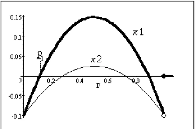
Example: There are n firms and demand is D (p) = max {0, 1 − p}. Costs are C (0) = 0 and C (q) = F ∈ (0, 1/4) for q > 0. With equal sharing, we have π1(p) = (1− p) p−F > πm(p) = (1− p) p/m−F whenever
π1(p) > 0 and for any m ∈ M, thus equal sharing is tie-decreasing. Since
π1 is llsc where it is positive and maximum profits are finite, by theorem 1
there are no Nash equilibria involving positive profits for any firm.
<< HERE FIGURE 2 >>
Assume that there is a zero-payoff equilibrium. The highest price p∗ such
that there are only countably many p ≤ p∗ with π1(p) > 0 is p∗ = p1 (see
Figure 2), thus from Lemma 3 it follows that t2 ≤ p1. Yet π1
³
p1´ = 0 and πm(p) < 0 for all p < p1 and all m ∈ N. Thus s ≥ p1 and α∗1
³ p1´ = α∗ 2 ³ p1´= 1, which contradicts πm ³ p1´< 0 for all m ∈ M.
On the other hand, pi = p1for all i ∈ N is a symmetric pure strategy
p < 1. As we will see below, the equilibrium exists because this sharing rule is sign-preserving.
Equilibria under SP sharing have simple structure:
Lemma 4 Given a Bertrand game Γ with SP sharing, in any Nash equilib-rium either J> = N and π1(p) > 0 for all p ∈ ∪i∈NPi, or J= = N and
π1(p) = 0 for all p∈ ∪i∈NPi with p < t1.
This lemma implies that we need not worry about atoms, since under SP sharing atoms cannot hide payoffs of opposite sign.
We make the following definitions:
Definition 4 1. An “initial viable price” (IVP) is a price s ∈ R+ such
that π1(s)≥ 0 and π1(p)≤ 0 for all p < s. If also π1(s) = 0 then s is
an “initial break-even price” (IBP, notion introduced by [3]).
2. A function f : R → R is right upper semi-continuous (rusc) at x ∈ R if lim supx0&xf (x0)≤ f (x).
An IVP is unique unless it is an IBP, and both IVP’s and IBP’s are natural candidates for symmetric pure strategy equilibria. The following theorem provides sufficient conditions for their existence and clarifies their relation with Nash equilibria under SP sharing.
Theorem 2 Given a Bertrand game Γ with SP sharing:
1. Assume that there is ¯p∈ R+ such that π1(¯p)≥ 0. An IVP exists if for
all p ∈ [0, ¯p] either π1 is rusc or non-negative.
3. Any IVP is an IBP if π1(0)≤ 0 and π1 is llsc.
4. Any IBP is unique if either π1 is strictly quasi-concave, or if π1 is
strictly increasing in an open neighborhood around any IBP.
5. There is a zero-payoff Nash equilibrium if and only if there is an IBP.
If payoffs π1 are not rusc then an IVP (and the corresponding Nash
equilibrium) may fail to exist: Let D (p) = 1−p, C (q) = q/2 for 0 ≤ q < 1/2, and C (q) = q for q ≥ 1/2, so that π1 is right-discontinuous at p = 1/2,
with π1(1/2) < 0. By Theorem 1 and Lemma 3 no Nash equilibria exist.
IVP’s form symmetric pure Nash equilibria under SP sharing simply because undercutting does not pay off.
Without left-continuity of π1 IBP’s may not exist: See the example of
Section 3, with c (q) slightly above 1/4 for q < 1/3. On the other hand, statement 4 indicates when IBP’s, and therefore symmetric pure strategy Nash equilibria with zero profits, are unique. This is the best uniqueness result that one can hope for, because if n > 2 then zero-payoff equilibria are always non-unique because some player can choose actions above t2 without
upsetting the equilibrium. Furthermore, we must still invoke theorem 1 to rule out equilibria with positive payoffs.
Statement 5 is a generalization of Theorem 1 in [3] on the relations be-tween IBP and zero-payoff equilibria. It depends decisively on the SP sharing assumption, which must be invoked for both the necessity and the sufficiency part ([3] invoke it for both without without stating it explicitly because they take the sharing rule as given). For arbitrary sharing rules the existence of an IBP is neither necessary nor sufficient for a zero-payoff equilibrium. The example at the beginning of this section shows the latter. The pure-strategy zero-payoff equilibrium pi = s, i ∈ N, with πn(s) = 0 > π1(s) in [5], under
the equal sharing rule and decreasing returns to scale, proves the former.
This theorem brings us back to the classical Bertrand result of zero profits. There is a change in intuition, however, which is that the classical “compet-itive outcome” of price equal to marginal cost is the exception rather than the rule, while the generic outcome is price equal to average cost. These two coincide only under constant returns to scale.
Finally, we remark how continuity of the demand and cost functions in the Bertrand model translates into the continuity of payoffs:
Lemma 5 Let the demand function D be non-increasing and the cost func-tion C be non-decreasing. If D and C are lower (upper) semi-continuous then π1 is right- (left-) continuous.
Interestingly, it is lower and not upper semi-continuity of demand that guarantees the existence of equilibria. The reason is that demand discon-tinuities pose no problems concerning existence unless they are magnified through the cost function into upward jumps in profits. Right-continuity at these upward jumps then follows from D being lower semi-continuous.
5
Expectation sharing rules
In this section we analyse a specific class of sharing rules in the Bertrand model, where π1(p) = pD (p)− C (D (q)). These sharing rules are obtained
by defining tied firms’ payoffs as the expected value of profits over some random distribution of quantities. In principle, the total quantity attributed could be different from the total quantity demanded, but we will concentrate on the case where they coincide. Under this restriction the quantities of tied firms are not independent random variables, therefore we will consider joint
distributions of quantities. Furthermore, since firms are symmetric we will only consider symmetric sharing rules.
First we need some definitions.
Definition 5 1. A joint distribution funtion Fp,m on [0, D (p)]m is a
sym-metric sharing distribution if the order of its arguments is irrelevant. An expectation sharing rule is a family F = {Fp,m}p∈R+,m∈M of sharing
distributions.
2. An expectation sharing rule is feasible if the supports of the joint prob-ability distributions Fp,m are contained in the sets
Fm(p) = n (q1, .., qm)∈ [0, D (p)]m ¯ ¯ ¯Xmi=1qi = D (p) o . (5)
In this case Fp,m is also called feasible. The sets of symmetric joint
probability distributions on Fm(p) are ∆ (Fm(p)). The set of feasible
and symmetric expectation sharing rules is E = ×p∈R+,m∈M∆ (Fm(p)).
A sharing rule {πm}m∈M is derived from F ∈ E by
πm(p) = E [pq− C (q) |p, m] =
Z
Fm(p)
[pq− C (q)] dFp,m(q, q2, .., qn) , (6)
for all p ∈ R+ and m ∈ M. The set E is larger than the set of sharing rules
{πm}m∈M, in the sense that for given (D, C) there may be several expectation
sharing rules F ∈ E that give rise to the same {πm}m∈M.
Expectation sharing rules have an interpretation in terms of demand com-position. A simple rule defines feasible distributions Fp,m for all pairs (p, m)
with:
• Equal sharing: The joint distributions Fp,m give weight 1 to the center
weight 1 to q = D (p) /m. Its interpretation is that infinitely many small buyers distribute themselves independently.
• Winner-take-all sharing W : The joint distributions Wp,m give weight
1/m to each of the m corner points (0, .., 0, D (p) , 0, .., 0) of Fm(p),
and the marginal distributions attribute weight (m − 1) /m at q = 0 and 1/m on q = D (p). [3] interpret this sharing rule as representing a single large buyer who randomly turns to one of the firms.
Other distributions of quantities follow from mixtures of buyers of differ-ent size.
Feasibility is a reasonable but not necessary requirement on expectation sharing rules.1 Alternatively one can imagine sharing rules where some
con-sumers “lose their way”, so that total demand faced by firms is less than D (p). Anyway, this notion has not appeared in the previous sections, so that the results obtained there do not depend on this assumption.
First we list some properties of expectation sharing rules:
Lemma 6 1. The set E of feasible and symmetric expectation sharing rules is convex. 2. If Fp,m ∈ ∆ (Fm(p)) for (p, m) ∈ R+× M then E [q|p, m] = D (p) /m and πm(p) = pD (p) m − E [C (q) |p, m] . (7) Expectation sharing rules need not be tie-decreasing, as the example of equal sharing shows. The following lemma presents an exact characterization, and a sufficient condition on C.
Lemma 7 Given (D, C), F ∈ E is tie-decreasing if and only if pD (p) < EhXm i=1C (qi) ¯ ¯ ¯ p, mi+ mπ1(p) (8)
for all m ∈ M and p ∈ R+ such that π1(p) > 0. All F ∈ E are tie-decreasing
if C is concave with C (0) = 0.
We will now determine when expectation sharing rules are sign-preserving. Given demand and cost functions D and C, denote the sets of zero-at-zero, or sign-preserving, feasible and symmetric expectation sharing rules as Ezaz(D, C)
and Esp(D, C), respectively. A generic element of these sets
has the form F = {Fp,m}p∈R+,m∈M. For any (D, C)
{W } ⊂ Esp(D, C)⊂ Ezaz(D, C)⊂ E. (9) In fact, we will consider an intermediate and two extreme versions of the above question:
1. For which class of demand and cost functions are all feasible and symmetric expectation sharing rules sign-preserving, i.e. Esp(D, C) =
E? 2. Which expectation sharing rules are sign-preserving for all demand and cost functions, i.e. which are the F ∈ E such that F ∈ Esp(D, C) for all
(D, C)? We already know that W is such a sharing rule.
3. For which demand and cost functions do sign-preserving expectation sharing rules exist that are different from the ones identified in question 2? That is, which are the (D, C) such that Esp(D, C)
6= {W }? The following Lemma provides the main tools for the analysis:
Lemma 8 1. Given demand and cost functions D and C, F ∈ Esp(D, C) if and only if, for all p ∈ R+ and m ∈ M,
pD (p)R EhXm
i=1C (qi)
¯ ¯
¯ p, mi if π1(p)R 0. (10)
2. Given demand and cost functions D and C, F ∈ Ezaz(D, C) if and
only if for all prices p0 such that π1(p0) = 0 we have, for all m∈ M,
EhXm i=1C (qi) ¯ ¯ ¯ p0, m i = C (q0) , (11)
where q0 = D (p0). The set Ezaz(D, C) is convex.
Conditions (8) and (10) demonstrate that the conditions of being tie-decreasing or sign-preserving are independent and do not contradict each other. More precisely, if a sharing rule is tie-decreasing and sign-preserving then EhXm i=1C (qi) ¯ ¯ ¯ p, mi< pD (p) < EhXm i=1C (qi) ¯ ¯ ¯ p, mi+ mπ1 (12)
for all m ∈ M and p ∈ R+ such that π1(p) > 0.
The convexity of the sets Ezaz(D, C) and Esp(D, C) implies that either they contain only the winner-take-all sharing rule W or they contain infinitely many elements.
Being zero-at-zero is a necessary condition for being sign-preserving. This is true even for profits π1 which do not have an IBP; in this case the
require-ment of being zero-at-zero is automatically fulfilled. As for the first of the above two questions, considering zero-at-zero sharing rules already provides a partial answer. Let P0 be the set of prices such that π1(p0) = 0, and P0+
the set of prices p0 ∈ P0 such that D (p0) > 0.
Lemma 9 Given any (D, C),
1. Ezaz(D, C) =
E if and only if, for all p0 ∈ P0 and m ∈ M,
Xm
2. if P0+ is empty then Ezaz(D, C) =
E; 3. if P0+ ={p0} then
(a) if n = 2, then Ezaz(D, C) =
E if and only if C (q) = cq + f (q) on [0, q0], where q0 = D (p0), c = p0 and f : [0, q0] → R is an
anti-symmetric function around q0/2 with f (0) = f (q0/2) = f (q0) =
0;
(b) if n > 2, then Ezaz(D, C) =
E if and only if C (q) = cq on [0, D (p0)], with c = p0.
4. If P0+ has more than one element, then Ezaz(D, C) $ E.
The power of the first point of this Lemma is that it reduces the condition in Lemma 8 to a simple restriction on the cost function. Point 2 states that if π1 has no zero then being zero-at-zero is a vacuous requirement on sharing
rules. Point 3a is driven by the symmetry between the two players, while in point 3b additional degrees of freedom rule out any deviations from linearity. The intuition of the fourth point is simple: Applying point 3 to two different prices p0 and p00 leads to a contradiction.
The previous lemma has also restricted the cases where Esp(D, C) =E. Clearly Esp
(D, C) $ E if P0+ has more than one element. If there are more
than two firms, we have:
Corollary 3 Let (D, C) be such that P0+={p0} and n > 2. If Esp(D, C) =
E then the cost function C is linear on [0, D (p0)].
Clearly Esp(D, L) =
E for any cost function L that is linear on [0, ∞), but the Corollary also allows for infinitely many cost functions that are non-linear above D (p0).
We will now turn to the case n = 2, and show that for most demand functions there exist non-linear cost functions such that Esp(D, C) =
E. The additional assumption that we must make is weak and can be relaxed if other functional forms are used in the construction.
Lemma 10 Let n = 2 and D be a non-increasing demand function. Assume that there is a price p0 where q0 = D (p0) > 0 and D is locally
Lipschitz-continuous: There are µ, ε > 0 such that |D (p) − D (p0)| < µ |p − p0| for all
p in an ε-neighborhood of p0. Then there are infinitely many cost functions
C such that Esp(D, C) =
E, of the form C (q) = cq + f (q), where c = p0 and
f (q) = ⎧ ⎨ ⎩ Aq³1 2 − q q0 ´ ³ 1−qq 0 ´ if 0≤ q ≤ q0 0 if q0 < q , for some A ∈ (−2ε, 0).
Now that we have answered the first question, the following lemma pro-vides us with a fast answer to the second question:2
Lemma 11 The only expectation sharing rule that is sign-preserving for all demand and cost functions is the winner-take-all sharing rule: If F ∈ E and F 6= W there are (D, C) such that F /∈ Esp(D, C).
The proof shows that W is the only sign-preserving expectation sharing rule if C is strictly convex or concave.
To answer the third question, the following lemma describes a weak suf-ficient condition on demand and cost such that W is not the only sign-preserving sharing rule.
Lemma 12 Assume that for (D, C) there is an IBP p0 with q0 = D (p0) and
for some m0 ∈ M there are q0, q00 ∈ Fm0(p0) with
Pm0
i=1C (qi0) > C (q0) and
Pm0
i=1C (qi00) < C (q0). Then there are infinitely many F ∈ Esp(D, C) with
F 6= W .
The condition on cost that drives this result can be interpreted as asking for sufficiently strong increasing returns to scale (Pm0
i=1C (qi0) > C (q0)) and
decreasing returns to scale (Pm0
i=1C (qi00) < C (q0)).
To sum up the preceding discussion: Winner-take-all sharing often is the only sign-preserving feasible and symmetric expectation sharing rule, but there is a large set of cases where either infinitely many or even all other such sharing rules are also sign-preserving.
6
Conclusions
We have analyzed Bertrand games from a different point of view. We did not take the distribution of payoffs at ties (the sharing rule) as given, but rather let it be the main object of analysis. To this effect we have deter-mined which properties of Bertrand equilibria depend on the sharing rule, and under which circumstances only zero-profit equilibria exist. We have shown that for the class of sign-preserving sharing rules (zero-profit) equi-libria exist under weak conditions, generalizing [3]. For other sharing rules the existence of equilibrium is not guaranteed. Finally, we have analised the class of expectation sharing rules, where payoff at ties is defined as expected profits over some random distribution of quantities.
On the conceptual level, the mode of analysis introduced in this paper may also be fruitful for the analysis of other games with discontinuous payoffs and equilibria involving ties with positive probability, for example auctions.
Furthermore, we believe that the relation between our approach and endoge-nous sharing rules points to a fruitful avenue for further research.
7
Appendix
Proof of Lemma 1:
1. Fix i ∈ N, and let pi be any point in Si, and φi ⊂ R+ any open
neighbor-hood around this point. The set φi∩ Si has positive mass under Fi∗, because
otherwise Si\φi would be a strictly smaller closed set containing probability
mass 1, a contradiction to Si being the smallest such set by definition. This
implies that φi∩ Si contains members of Pi. Since this is true for all points
pi and neighborhoods φi, the set Pi is dense in Si for all i ∈ N.
For i ∈ N, let G∗
i (p) = 1− Fi∗(p) + α∗i (p) = Pr (pi ≥ p), which is
left-continuous in p. Clearly, max {α∗
i (p) , 1− Fi∗(p)} ≤ G∗i (p) ≤ 1 for all p ∈
R+, and limp→∞G∗i (p) = 0. From (2), for all i ∈ N and p ∈ R+,
u¡p, F−i∗ ¢≤ X T ⊂Ni ¯ ¯π|T |+1(p)¯¯Y j6=i G∗j(p)≤ 2n−1πmaxY j6=i G∗j(p) (14) thus limp→∞u¡p, F∗ −i ¢
= 0. For all i ∈ J> the support Si must therefore
have a finite maximum ti, and sup Pi = ti because Pi is dense in Si. Let
t = mini∈J>ti. If there is any j ∈ J> with tj > t, we have uj
¡ p, F∗
−j
¢
= 0 for all p ∈ (t, tj] since G∗i (p) = 0 for at least one firm i with ti = t. This is a
contradiction to sup Pj = tj, thus tj = tfor all j ∈ J>.
By (14), for every i ∈ N lim sup p%t u¡p, F−i∗ ¢≤ 2n−1πmaxY j6=i lim p%tG ∗ j(p) = 2n−1πmax Y j6=i G∗j(t) .
If there is any j ∈ Nisuch that G∗j(t) = 0this implies that lim supp%tu
¡
p, F−i∗ ¢ ≤ 0, which is a contradiction to Πi > 0 and sup Pi = t if i ∈ J>. Therefore
G∗
j(t) > 0 for all j ∈ Ni if i ∈ J>, which implies Fj∗(t) < 1 + α∗j (t) for
all j ∈ J=, and t ∈ Pj and α∗j(t) > 0 for all j ∈ J>\ {i} if |J>| > 1. The
statement for J>={i} follows from the proof in the next paragraph applied
to t = sup Pi. Note that in this case we cannot conclude that t ∈ Pi.
For any two firms j, k ∈ N, j 6= k, we can write firm j’s expected profits at price p as u¡p, F−j∗ ¢ = α∗k(p) Ujk(p, 2) + (1− Fk∗(p)) Ujk(p, 1) , (15) where, with Njk= N\ {j, k}, Ujk(p, a) = X T ⊂Njk π|T |+a(p)Y i∈T α∗i (p)× Y l∈Njk\T (1− Fl∗(p)) . Since at p = t we have 1 − F∗ j (t) = 0 if j ∈ J>, it follows that u ¡ t, F∗ −k ¢ = α∗ j(t) Ujk(t, 2) for any k ∈ Ni. If k ∈ J> then u ¡ t, F∗ −k ¢ = Πk and u ¡ t, F∗ −j ¢ = α∗ k(t) Ukj(t, 2) = Πj,
from which follows α∗
k(t) Πk = α∗j (t) Πj since Ujk(p, a) = Ukj(p, a). Since
the pairing (j, k) was arbitrary, α∗
i (t) Πi = K for all i ∈ J> and some K > 0.
If on the other hand k ∈ J= and α∗j(t) > 0, which is definitely true if
|J>| > 1, then necessarily Ujk(t, 2) ≤ 0. Since α∗k(t) = 0 if Ujk(t, 2) < 0, in
any case α∗ k(t) Ujk(t, 2) = 0, and u ¡ t, F∗ −j ¢ = (1− F∗ k (t)) Ujk(t, 1) = Πj > 0,
from which follows that 1 − F∗
k(t) > 0.
2. Assume now that J= 6= ∅, and that for some firm j ∈ J> the set Pj is
uncountable. Since all Si, i ∈ N, can contain only countably many atoms,
Pj then contains a price ˆp < t such that α∗j(ˆp) = α∗k(ˆp) = 0 for some firm
k ∈ J=. Payoffs at this price are
uj ≡ u ¡ ˆ p, F−j∗ ¢= (1− Fk∗(ˆp)) Ujk(ˆp) , uk ≡ u ¡ ˆ p, F−k∗ ¢ =¡1− Fj∗(ˆp) ¢ Ujk(ˆp) .
Since F∗
j (ˆp) < 1, uj = Πj > 0and uk ≤ 0 contradict each other. The sets Pj,
j ∈ J>, are therefore countable, and can contain only atoms and a countable
number of limit points of atoms. These atoms contain all probability mass. The sets Sj, j ∈ J>, do therefore not contain any open sets without atoms.
It also follows from the above argument that any price p < t in Pj, for
some firm j ∈ J>, and which is not an atom for firm j, must be an atom for
all firms i ∈ J=.
Finally, any price p < t which is not an atom for any firm gives rise to positive profits if π1(p) > 0. Therefore in an equilibrium with J= 6= ∅ this
price must either be an atom of some firm in J>, or of at least two firms in
J=.
Proof of Lemma 2:
1. For each p ∈ Pi for some i ∈ J> it follows from u
¡ p, F∗ −i ¢ > 0 that Q j6=iG∗j(p) > 0. Letting R∗il(p) = X T ⊂Ni |T |=l−1 Y j∈T α∗ j(p) G∗ j(p) × Y k∈Ni\T µ 1− α ∗ k(p) G∗ k(p) 
for all l ∈ N and p ∈ Pi, we can write payoffs (2) as
u¡p, F−i∗ ¢=Y j6=i G∗j(p)× n X l=1 R∗il(p) πl(p) .
The term R∗il(p) is the probability that (l − 1) firms are tied with firm i
at price p, given that all firms j ∈ Ni choose prices greater or equal than
p. Then 0 ≤ R∗il(p) ≤ 1 and
Pn
l=1R∗il(p) = 1. Therefore, the expression
Pn
l=1R∗il(p) πl(p) is a weighted average of {π1(p) , .., πn(p)}, and is strictly
positive since p ∈ Pi.
As in ∪j6=iSj there are only countably many atoms there is an increasing
By underbidding p slightly, firm i can guarantee itself, in the limit, at least the payoff lim infl→∞π1(pl) Y j6=i Gj(pl) = Y j6=i Gj(p) lim infl→∞π1(pl) ≥ Y j6=i Gj(p) lim infp0%pπ1(p0) .
Since p ∈ Pi it is necessary that Pnl=1R∗il(p) πl(p) ≥ lim infp0%pπ1(p0). If π1
is llsc at p if follows that Pnl=1Ril∗(p) πl(p) ≥ π1(p).
Now if A∗(p, N ) ≥ 2 then there is j ∈ N
i such that α∗j(p) > 0, and thus
R∗
i1(p) < 1. It follows that there is an m ∈ M such that πm(p) > 0 and
πm(p)≥ π1(p).
On the other hand, if J= 6= ∅ then by Lemma 1 necessarily π1(p) ≤ 0
for almost all prices p < t since there are only countably many atoms in ∪i∈NSi. Therefore lim infp0%¯pπ1(p0) ≤ 0 for all ¯p < t. If π1 is llsc at p ∈ Pi
then π1(p) ≤ 0, from which follows that there is an m ∈ M such that
πm(p) > 0≥ π1(p) since
Pn
l=1R∗il(p) πl(p) > 0.
Proof of Lemma 3:
First note that s = min ∪i∈NSi exists since all Si are closed and bounded
from below.
1. It is clear that π1(p)≤ 0 for all p < s because otherwise a deviation
to a p with π1(p) > 0 would lead to positive payoffs. Since there are only
countably atoms in ∪i∈NSi, almost all p < t2 yield player 1 u
¡ p, F∗ −1 ¢ = π1(p) Q j∈N1 ¡ 1− Fj∗(p) ¢
, which is positive unless π1(p) ≤ 0. On the other
hand, if π1(p) > 0 then A∗(p, N1) > 0, and there is m ∈ M such that
πm(p)≤ 0.
2. For i ∈ N let p ∈ Pi with p < t1. Then G∗j(p) > 0 for all j ∈ Ni, and
Pn
k=1Rik∗ (p) πk(p) = 0, and there is m ∈ M with πm(p)≥ 0 if π1(p) < 0.
Proof of Lemma 4:
Let i ∈ J> 6= ∅ and j ∈ J= 6= ∅. Since u
¡ p, F∗
−i
¢
> 0 for p ∈ Pi, SP sharing
implies that πm(p) > 0, m ∈ N. Thus u
¡ p, F∗ −j ¢ > 0, a contradiction. If J= = N then u ¡ p, F∗ −i ¢
= 0 for p ∈ Pi implies πm(p) = 0 for all m ∈ N if
p < t1.
Proof of Theorem 2:
1. Define p∗ ≤ ¯p as p∗ = inf{0 ≤ p ≤ ¯p|π
1(p) ≥ 0}. Either π1(p∗) ≥ 0,
or by upper semi-continuity from the right we must have 0 ≤ lim supp&p∗
π1(p) ≤ π1(p∗). By definition of p∗, π1(p) < 0 for all p < p∗, thus p∗ is an
IVP.
2. If p is an IVP, by SP sharing πn(p)≥ 0. Playing p with probability 1
is a pure symmetric equilibrium since uncercutting does not increase payoffs. 3. Let p0 > 0 be an IVP. Since π1 is llsc at p0:
0≥ lim
p%p0
inf π1(p)≥ π1(p0)≥ 0,
i.e. π1(p0) = 0. If p0 = 0 is an IVP then π1(0) ≥ 0 by definition. By
assumption π1(0)≤ 0, so again π1(p0) = 0.
4. Let pl< ph be IBP’s. If π1 is strictly quasi-concave then π1(p) > 0for
all p ∈ (pl, ph). If π1 is strictly increasing in an open neighborhood around
pl, then there are an ε ∈ (0, ph− pl) and p ∈ (pl, pl+ ε) with π1(p) > 0.
Both contradict ph being an IBP.
5. An IBP p is an IVP with π1(p) = 0 and leads to a zero-payoff Nash
equilibrium by point 2. For the converse, assume there is a zero-payoff Nash equilibrium with firms ordered such that t1 ≤ .. ≤ tn. For any p ∈ P1,
u¡p, F−1∗ ¢= 0 and by SP sharing π1(p) = 0. By Lemma 3, π1(r)≤ 0 for all
r ∈ [0, s). Any p ∈ [0, t1] with π1(p) > 0 would lead to u
¡ p, F∗
−1
¢
> 0under SP sharing, thus π1(p)≤ 0 for all p ∈ [0, t1]. Since P1 ⊂ [s, t1]is non-empty
Proof of Lemma 5:
Let D and C be lower semi-continuous. Since D is non-increasing and C is non-decreasing, D is right- and C is left-continuous. Therefore π1 is
right-continuous. The analogous result holds if D and C are upper semi-continuous.
Proof of Lemma 6:
Given any (p, m) ∈ R+×M, if Fp,m, Gp,m ∈ ∆ (Fm(p))then for any λ ∈ [0, 1]
the function λFp,m + (1− λ) Gp,m is also a symmetric and feasible sharing
distribution on Fm(p). As for the second statement, by symmetry and
fea-sibility we obtain, for any (p, m) and i ∈ {1, .., m}, mE [q|p, m] =Xm i=1E [qi|p, m] = E hXm i=1qi ¯ ¯ ¯ p, mi= E [D (p)|p, m] = D (p) . Proof of Lemma 7:
If (q1, .., qm)∈ Fm(p)then by symmetry mE [C (q) |p, m] = E [Pmi=1C (qi)|p, m],
so πm = 1 m ³ pD (p)− EhXm i=1C (qi) ¯ ¯ ¯ p, mi´.
The statement then follows from π1(p) > πm(p) whenever π1(p) > 0.
Re-arranging terms differently leads to
π1(p) > 1 m− 1 ³ C (D (p))− EhXm i=1C (qi) ¯ ¯ ¯ p, mi´. (16) If C is concave with C (0) = 0 then C (q) /q ≤ C (λq) /λq for any q > 0 and λ ∈ (0, 1). For 0 < q1 ≤ q2 it follows that
C (q1+ q2)≤ (q1+ q2) C (q2) q2 ≤ q 1 C (q1) q1 + q2 C (q2) q2 = C (q1) + C (q2) ,
which also holds if q1 = 0. By induction, C (D (p)) = C (Pmi=1qi) ≤
Pm
i=1C (qi) for any (q1, .., qm) ∈ Fm(p). This makes the right-hand side
of (16) non-positive.
Proof of Lemma 8:
By definition, the sharing rule F = {Fp,m}p∈R+,m∈M ∈ E is sign-preserving if,
for all p ∈ R+ and m ∈ M, E [pq − C (q) |p, m] R 0 if π1(p) R 0. By Lemma
6, and summing over i = 1, .., m we obtain the result. Let {Fp,m} , {Gp,m} ∈
Esp
. Then for any λ ∈ [0, 1] and all p ∈ R+ and m ∈ M,
EλFp,m+(1−λ)Gp,m[.] = λEFp,m[.] + (1− λ) EGp,m[.] .
As concerns the second statement, it follows immediately from the first state-ment and π1(p0) = p0D (p0)− C (q0) = 0.
Proof of Lemma 9:
1. If Pmi=1C (qi) = C (q0)∀ q ∈ Fm(p0) for all p0 ∈ P0 and m ∈ M, then for
any F ∈ E EhXm i=1C (qi) ¯ ¯ ¯ p0, m i = E [ C (q0)| p0, m] = C (q0) ,
and by Lemma 8 F ∈ Ezaz(D, C). For the reverse, consider some p 0 ∈ P0
and some m0 ∈ M such that there is a q0 ∈ F
m0(p0)with
Pm0
i=1C (q0i) = K 6=
C (q0). Let Fp0,m0 be the sharing distribution that gives equal weight to all
permutations of q0 and zero weight to the rest of F
m0(p0). Then clearly E∙Xm 0 i=1C (qi) ¯ ¯ ¯ ¯ p0, m0 ¸ = K 6= C (q0) ,
and the resulting expectation sharing rule is not zero-preserving.
2. This point is obvious since being zero-at-zero implies no restriction in this case.
3a. Assume that C (q) = cq + f (q) as described in the statement. Then for any (q1, q2)∈ F2(p0) we have q2 = q0− q1 and
C (q1) + C (q0− q1) = cq0+ f (q1) + f (q0− q1)
= cq0 = C (q0) .
For the converse, let c = C (q0) /q0 and f (q) = C (q) − cq on [0, q0], which
implies f (q0) = 0. For any point (q1, q0− q1)∈ F2(p0) it follows that
C (q1) + C (q0− q1) = cq0+ f (q1) + f (q0− q1) .
Condition 13 can only be fulfilled if f (q1) + f (q0− q1) = 0. If this is to be
true for all q1 ∈ [0, q0] it implies that f is anti-symmetric around q0/2 and
that f (0) = f (q0/2) = 0. This proves statement 3a.
3b. Clearly Ezaz(D, C) =
E if C (q) = cq on [0, D (p0)]because
Pm
i=1C (qi) =
cPmi=1qi = cq0. Now for the converse. Given the result of point 3a we will
prove that f (q) = 0 on [0, q0] once we allow m > 2. Consider m = 3. Then
for any point (q1, q2, q3)∈ F3(p0),
X3
i=1C (qi) = cq0+
X3
i=1f (qi) .
Condition 13 then implies that P3i=1f (qi) = 0 for any (q1, q2, q3)∈ F3(p0).
Letting δ ∈ [0, q3]we arrive at two more identities:
f (q1+ δ) + f (q2) + f (q3− δ) = 0,
f (q1) + f (q2+ δ) + f (q3− δ) = 0.
Taking differences leads to
f (q1+ δ)− f (q1) = f (q2+ δ)− f (q2) .
Since q1, q2 and δ are arbitrary this means that the function f must have
a constant slope, which given f (0) = f (q0) = 0 is only possible if f is
4. Let p1, p2 ∈ P0+ with p1 < p2 and note that point 3a of this Lemma
applies to both p1 and p2. Let m = 2 and assume that C (q) = cq + f (q) on
[0, D (p1)]with f (D (p1)) = f (D (p2)) = 0. Then π1(pi) = (pi− c) D (pi) =
0 implies p1 = p2 = c, a contradiction.
Proof of Lemma 10: Choose ε such that ε ≤¡12 −
1 6
√ 3¢q0
µ. We will proceed in four steps.
1. Identify a sufficient condition on f which is independent of the sharing rule.
Fix an expectation sharing rule F ∈ E. For F ∈ Esp(D, C) we must have
(p− c) D (p) T E [f (q) + f (D (p) − q) |p, 2] ∀ p T p0. Let ¯ g (q) = max 0≤z≤q{f (z) + f (q − z)} , g (q) = min0≤z≤q{f (z) + f (q − z)} , then g (D (p)) ≤ E [f (q) + f (D (p) − q) |p, 2] ≤ ¯g (D (p))
because the distributions Fp,2 are symmetric. Therefore it is sufficient for
F ∈ Esp(D, C)if both
(p− c) D (p) > ¯g (D (p)) ∀p > p0,
(p− c) D (p) < g (D (p)) ∀p < p0.
2. Compute the functions ¯g and g.
If q < q0 then the maximum of f (z) + f (q − z) is attained at z = 0, with
¯ g (q) = f (q) = Aq µ 1 2− q q0 ¶ µ 1− q q0 ¶ .
For q > q0, the minimum of f (z) + f (q − z) is attained at z = q − q0, with g(q) = ⎧ ⎨ ⎩ g1(q) =−3 ³ 1−qq 0 ´ ³ 1− 23qq 0 ´ ³ 1−2qq 0 ´ Aq0 if q≤ ¡3 2 − 1 6 √ 3¢q0 g2(q) = 121√ 3Aq0 if q > ¡3 2 − 1 6 √ 3¢q0 . 3. Show that (p − c) D (p) > ¯g (D (p)) ∀p > p0
We have D (p) ≥ D (p0) − µ (p − p0) > 0 (because ε < qµ0) for p ∈
(p0, p0+ ε). Let l (q) = p0 + ε−qεq0 with l (q0) = p0 and l (0) = p0+ ε. Then
(p− c) D (p) ≥ (l (D (p)) − c) D (p), and (l (q)− c) q = ε µ 1− q q0 ¶ q > ¯g (q) = Aq µ 1 2 − q q0 ¶ µ 1− q q0 ¶ if 1 > A ε ³ 1 2 − q q0 ´
. Sufficient for this is 1 > −1 2 A ε or A > −2ε. 4. Show that (p − c) D (p) < g (D (p)) ∀p < p0. Since A > −2ε, we have A > −2ε¡3 +√3¢≥ −2q0 µ since ε ≤ ¡1 2 − 1 6 √ 3¢q0 µ. Then, for p ∈ (p0− ε, p0), D (p) < D (p0)− µ (p − p0) < D (p0) + 2 q0 A (p− p0) , (p− c) D (p) < (p − c) q0 <− A 2 µ 1− D (p) q0 ¶ q0 ≤ g1(q) .
We must check that indeed q = D (p0− ε) ≤
¡3 2 − 1 6 √ 3¢q0, which is true since D (p0− ε) ≤ D (p0) + µε≤ µ 3 2− 1 6 √ 3 ¶ q0. Now for p < p0− ε (p− c) D (p) < (p0− ε − c) D (p0− ε) ≤ −εq0 < g2(q)
if A > −12√3εwhich is weaker than A > −2ε. Proof of Lemma 11:
Consider demand and cost functions D and C which give rise to an IBP p0. Furthermore, assume that C is strictly convex with C (0) = 0. For any
(q1, .., qm) ∈ Fm(p0), we have Pmi=1qi = q0. On the other hand, since C
is strictly convex with C (0) = 0 then Pmi=1C (qi) < C (q0) unless there
is some j ∈ {1, .., m} such that qj = q0 and qi = 0 for all i 6= j. In
this case Pmi=1C (qi) = C (q0) holds. That is, equality is only obtained
at the m corner points of Fm(p0), therefore by Lemma 8 all probability mass
must be concentrated there. By symmetry, each corner point has a mass of 1/m, which is the probability distribution of the winner-take-all sharing rule. Therefore only W is in Ezaz(D, C)
, and by implication in Esp(D, C).
Proof of Lemma 12:
For simplicity, we will construct a set of sharing rules in Esp(D, C)different
from W only at (p0, m0). Let Fp,m be equal to the winner-take-all sharing
distribution for all (p, m) ∈ R+×M\ {(p0, m0)}. Let F0,F00 ∈ ∆ (Fm0(p0))be
the two sharing distributions that attribute equal weight to all permutations of the tuples q0 and q00, respectively. Then for F0,
EF0 hXm0 i=1C (qi) ¯ ¯ ¯ p0, m0 i =Xm0 i=1C (q 0 i) ,
with the corresponding result for F00. Let
λ = C (q0)− Pm0 i=1C (qi00) Pm0 i=1C (qi0)− Pm0 i=1C (q00i) ∈ (0, 1) ,
and define Fp0,m0 = λF0+ (1− λ) F00, which is also a member of ∆ (Fm0(p0))
because it is a convex set. Then
EFp0,m0 hXm0 i=1C (qi) ¯ ¯ ¯ p0, m0 i = λEF0 hXm0 i=1C (qi) ¯ ¯ ¯ p0, m0 i + (1− λ) EF00 hXm0 i=1C (qi) ¯ ¯ ¯ p0, m0 i = λXm0 i=1C (q 0 i) + (1− λ) Xm0 i=1C (q 00 i) = C (q0) ,
which implies that Fp0,m0 is zero-at-zero and F ∈ E
sp(D, C)
\ {W }. Since Esp(D, C) is convex, any convex combination between F and W is also a
References
[1] Balder, E. J.: On Equilibria for Discontinuous Games: Continuous Nash Approximation Schemes. mimeo, Mathematical Institute, University of Utrecht (March 2002)
[2] Baye, M. R., Morgan, J.: A Folk Theorem for One-Shot Bertrand Games. Economics Letters 65, 59—65 (1999)
[3] Baye, M. R., Morgan, J.: Winner-take-all Price Competition. Economic Theory 19, 271-282 (2002)
[4] Dasgupta, P., Maskin, E.: The Existence of Equilibrium in Discontinu-ous Economic Games, I:Theory. Review of Economic Studies 53, 1—26 (1986)
[5] Dastidar, K. G.: On the Existence of Pure Strategy Bertrand Equilib-rium. Economic Theory 5(1), 19—32 (1995)
[6] Harrington, J. E.: A Re-Evaluation of Perfect Competition as the Solu-tion to the Bertrand Price Game. Mathematical Social Sciences 17(3), 315—328 (1989)
[7] Hoernig, S. H.: Mixed Bertrand Equilibria under Decreasing Returns to Scale: An Embarrassment of Riches. Economics Letters 74(3), 359—62 (2002)
[8] Kaplan, T.R., Wettstein, D.: The Possibility of Mixed-Strategy Equi-libria with Constant-Returns-to-Scale Technology under Bertrand Com-petition. Spanish Economic Review 2(1), 65—71 (2000)
[9] Osborne, M. J., Pitchik, C.: Price Competition in a Capacity-Constrained Duopoly. Journal of Economic Theory 38, 238-260 (1986)
[10] Reny, P. J.: On the Existence of Pure and Mixed Strategy Nash Equi-libria in Discontinuous Games. Econometrica 67(5), 1029—56 (1999)
[11] Sharkey, W. W., Sibley, D. S.: A Bertrand Model of Pricing and Entry. Economics Letters 41(2), 199—206 (1993)
[12] Simon, L. K., Zame, W. R.: Discontinuous Games and Endogenous Sharing Rules. Econometrica 58(4), 861—72 (1990)
[13] Sion, M., Wolfe, P.: On a Game Without a Value, Annals of Mathemat-ics Studies 39, 299—306 (1957)
[14] Vives, X.: Oligopoly Pricing: Old Ideas and New Tools. Cambridge, MA: MIT Press 1999
Figure Legends:
Figure 1: One firm may make positive equilibrium profits.
Figure 2: No pure or mixed equilibria because of increasing returns to scale and equal sharing.