José Pedro Pontes (ISEG/UTL and UECE)
January 2006
Abstract
This paper models the decision of vertically-linkedfirms to build either partitioned or connected networks of supply of an intermediate good. In each case, the locations of upstream and downstream firms are correlated. Input specificity is related both to variable costs (transport costs of the input) andfixed costs (learning costs of the use of the input). When both are low, a connected network emerges and a partitioned pattern arises in the opposite case. In the boundary region, there are multiple equilibria, either asymmetric (mixed network) or symmetric.
K eyw ords: Location, Vertically-linked industries, Intermediate goods, Networks, Inputflexibility
JE L classification: R30, L13
Address: Instituto Sup erior de Economia e Gestão, Rua M iguel Lupi, 20, 1249-078 Lisb oa Portugal.
Tel. 351 21 3925916
Fax 351 21 3922808
Em ail<pp ontes@iseg.utl.pt>
The author wishes to thank André Rocha and Armando Pires for their helpful comments. The usual
disclaimer applies. This article had the supp ort of the Research Unit on Complexity in Economics
1. Introduction
The issue of the flexibility of an intermediate good concerns the choice that a supplier makes between either producing a specialized input exactly tailored to the needs of a given buyer or manufacturing a generic or standardized input that can be used by all or at least by several buyers. In spatial terms, if the sellers and buyers of the intermediate good are defined by addresses in an attribute space, the specialization strategy amounts to the input supplier competing locally in its neighborhood, while the generic strategy is equivalent to competing globally in the whole attribute space.
This issue is important on two grounds. Thefirst is the relationship between input specificity and the incentive to vertical integration, which was established by Williamson (1981) and Joskow (1987). Under input specificity, an incentive to a long-term bilateral relationship between buyer and seller is created, which can be best governed (in the sense of minimizing transaction costs) in the context of vertical integration rather than through the open market. Although this is an important strand in the literature, the focus on the importance of input specificity in this paper will lie elsewhere.
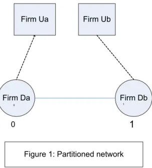
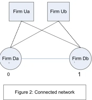
decide to produce generic inputs, each supplier will sell to several buyers and each buyer will procure the input from several sellers, so that a connected network will emerge, in which each node (firm) has at least two connections. The structure of the network matters because a partitioned structure implies an interdependence between the industrial dynamics at the upstream and downstream levels that is closer than the one found in the connected structure.
The choice of the degree of specialization of an input is usually regarded as the outcome of a trade-off between economies of scale (which are maximized under the standardization of the input) and adjustment costs (which are minimized if the inputs are specialized, see Lorz and Wrede, 2005). A generic input can be produced in large amounts, thus savingfixed costs, but on the other hand must be adapted to the specific needs of the users. These adaptation costs can be viewed as transport costs in relation to the distance between the seller and buyer’s addresses in the attribute space.
This paper seeks to model the adjustment costs of the intermediate good, us-ing the spatial framework. We assume that the transport cost of the intermediate good in the distance between the seller and the buyer’s addresses is the variable component of the adjustment cost, as mentioned by the literature onflexible man-ufacturing systems (see Eaton and Schmitt, 1994; Norman and Thisse, 1999) and on the endogenous choice of the degree of input specificity (see Pontes, 2005). Furthermore, following Kranton and Minehart (2000), it is argued that inputfl ex-ibility has not only a variable cost, but also afixed cost. In order to sell the input, the upstreamfirm has to train the buyer to use it, and this learning cost has the nature of afixed cost.
2. The model
2.1. Assumptions
The paper models a spatial economy that obeys the following assumptions:
1. The consumers are uniformly distributed with unit density in the space de-scribed by the interval[0,1]. Each consumer has an inverse demand function p= 1−q.
2. Two downstreamfirms, Da andDb, supply a consumer good in the market
space. Thesefirms havefixed locations at the end points of the market:Da
locates in0andDb locates in1. They compete in quantities at each point
of the market and they transport and deliver the product to the consumers. The transport cost of one unit of the consumer good per unit of distance is given byt∈(0,1).
3. Two upstream firms Ua and Ub have variable locations sa and sb in [0,1].
They compete in quantities in the markets represented by downstreamfirms Da and Db and they transport and deliver the intermediate good. The
transport cost of the intermediate good per unit of distance is given byτ.
4. The downstreamfirms transform one unit of intermediate good in one unit of consumer good and the cost of the intermediate good is their only variable cost.
5. Each upstreamfirm can choose to supply to either one or both downstream
It is assumed that this cost is borne by the seller of the intermediate good. Without loss of generality, it is assumed that, iffirm Ua (respectively, Ub)
sells to a single buyer, it selectsfirmDa(firmDb, respectively).
2.2. The game structure
We assume that thefirms play a four stage game:
First Stage Each upstream firm decides to sell to one or to two input buyers. As a consequence, a network is formed with one of four different types: a partitioned structure, where eachfirm has a single connection; a connected structure, where eachfirm has two connections; and two mixed structures, where an upstream-downstream pair offirms has two connections, with the remainingfirms having a single connection (see Figures 1, 2 and 3).
Second Stage The upstream firms simultaneously select locationssa and sb in
[0,1].
Third Stage The upstreamfirms select quantities of the intermediate goodxaa,xab,xba,xbb, where, for instance,xabis the quantity of input sold byfirmUatofirmDb.
xabandxbacan be zero, depending on the the outcome of thefirst stage of the game.
Fourth Stage The downstream firms Da and Db choose quantities qa(r) and
qb(r)to be sold at each point of the marketr∈[0,1].
(Insert here Figures 1,2,3)
point of the market. Their profits on sales in pointr∈[0,1]are:
πDa(r) = [(1−(qa+qb)−wa−tr)]qa (1)
πDb(r) = [(1−(qa+qb)−wb−t(1−r))]qb (2)
whereqaandqbare the quantities andwaandwbare the prices of the intermediate
good in the downstreamfirms’ locations. The Nash equilibrium quantities are:
qa(r) =
1
3t−rt− 2 3wa+
1 3wb+
1
3 (3)
qb(r) = rt−
2 3t+
1 3wa−
2 3wb+
1
3 (4)
In order to solve the third-stage game, it is necessary to consider separately the networks that follow from thefirst stage and are depicted in Figures 1, 2 and 3.
The following proposition summarizes thefindings (see proof in Appendix A):
Proposition 1 In the partitioned network case (Figure 1), the Nash equilibrium
quantities of the input are
xaa = 1
15τ− 1 10t−
4 15τ sa−
1 15τ sb+
1
5 (5)
xbb = 1
15τ sa− 4 15τ−
1 10t+
4 15τ sb+
1
5 (6)
Nash equilibrium quantities of the input are
xaa = 1
9τ− 1 18t−
2 3τ sa+
1 3τ sb+
1
9 (7)
xab = 2
3τ sa− 2 9τ−
1 18t−
1 3τ sb+
1
9 (8)
xba = 1
9τ− 1 18t+
1 3τ sa−
2 3τ sb+
1
9 (9)
xbb = 2
3τ sb− 2 9τ−
1 3τ sa−
1 18t+
1
9 (10)
In the mixed network case (Figure 3-a), the Nash equilibrium quantities of the
input are given by
xaa = 1
6τ− 1 12t−
1 2τ sa+
1
6 (11)
xab = 7
12τ sa− 1 4τ−
1 24t−
1 6τ sb+
1
12 (12)
xbb = 1
3τ sb− 1 6τ−
1 6τ sa−
1 12t+
1
6 (13)
and xba = 0by assumption. The Nash equilibrium quantities of the input in the
mixed network case of Figure 3-b are symmetric to 11, 12 and 13.
It is also simple to show the following proposition (see proof in Appendix B):
Proposition 2 In each network structure, the Nash equilibrium locations of the
upstream firms entail the location of an input supplier alongside an input buyer
(i.e. sa= 0, sb= 1) in order to save the transport costs of the intermediate good.
Substituting the locations of proposition 2 into 8, 9 and 12, it is easily concluded that the feasibility of connections between spatially separatedfirms (i.e. xab>0
and xba>0) implies that the transport cost of the input is bounded from above
τ < 1
5− 1
From 3, 4 and proposition 1, it can be concluded that the condition
t < 2
7(1 +τ) (15)
together with condition 14 ensures that each downstream firm located at an ex-treme point of the interval[0,1]sells a positive amount of the consumer good at each point of the market for any network structure.
The co-location of the suppliers and buyers of the input is not sensitive to the network structure. However, it should be noticed that:
Remark 3 Although co-location of input supplier and buyer holds in each network
structure, the robustness of the equilibrium decreases with the degree of connectivity
of the network. With a partitioned network, co-location is a dominating strategy
equilibrium. With a mixed network, it is a unique Nash equilibrium. With a fully
connected network, there are two co-location Nash equilibria.
Hence, there is a close relationship between the location of the upstream and downstreamfirms. However, the robustness of this correlation decreases with the degree of connectedness of the network, confirming thefindings of Bonaccorsi and Giuri (2001).
Inputflexibility is expressed inversely by the unit transport cost of the input and by thefixed cost entailed by establishing a connection between a supplier and a buyer of the intermediate good.
πUa(1,1) = πUb(1,1) =
1 50t
2
−252t−c+ 2 25
(16)
πUa(2,1) = πUb(1,2) =
5 72tτ−
7 72t−
5
36τ−2c+ 7 288t 2 +19 72τ 2 + 7 72 (17)
πUa(1,2) = πUb(2,1) =
1 9τ−
1
18t−c− 1 18tτ+
1 72t 2 + 1 18τ 2 + 1 18 (18)
πUa(2,2) = πUb(2,2) =
1 27tτ−
2 27t−
2
27τ−2c+ 1 54t 2 +14 27τ 2 + 2 27 (19)
The game expressed by these payofffunctions is a symmetric two-person game. Let us define
A1 = πUa(1,1)−πUa(2,1)
A2 = πUa(2,2)−πUa(1,2)
Then, the signs of A1 and A2 completely determine the equilibrium of the game. It is easy to see that
A1 > 0⇔c >
5 72tτ−
5 36τ−
31 1800t+
31 7200t 2 +19 72τ 2 + 31
1800 ≡F(t, τ)
(20)
A2 > 0⇔c <
5 54tτ−
5 27τ−
1 54t+
1 216t 2 +25 54τ 2 + 1
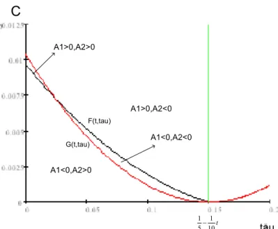
For given values oft, F(t, τ) and G(t, τ) define two convex parabolas in τ. F(t, τ) has two roots, namely τ = 1
5 − 1
10t and τ = 31 95 −
31
190t, the former root being smaller than the latter fort∈(0,1). G(t, τ)has a single rootτ =1
5 − 1 10t. Given boundary condition 14, only values of (t, τ), such thatτ < 1
5 − 1
10t, have any economic meaning. In this region, F(t, τ)andG(t, τ)intersect twice.
F(t, τ) =G(t, τ)⇔τ= 7 215−
7
430t∨τ = 1 5−
1
10t (22)
It is clear that in 22, the first root is positive and strictly smaller than the second root fort∈(0,1). Summing up, it is possible to plot condition 14 and 20 and 21 in the space (τ , c)in Figure 4 (a valuet= 0.5is implicitly assumed in this
figure, but thefigure is not sensitive to the specific value oft,provided that this value is feasible according to conditions 14 and 15).
(Insert here Figure 4)
Figure 4 shows that, for high values of the transport cost of the intermediate good and for high connection costs, to compete locally, i.e. to supply only the nearby buyer, is a dominating strategy for both upstream firms. By contrast, if τ and care low, it is a dominating strategy for both input suppliers to compete globally, i.e. to supply both downstreamfirms.
decides to compete globally, the best reply is to compete locally and vice-versa. A mixed network as depicted in Figure 3 emerges. It should be noticed that:
Remark 4 For any value of t, the region where the connection game has
multi-ple asymmetric equilibria is much larger than the region with multimulti-ple symmetric
equilibria. Whenever there is no dominating strategy, the connection game is more
likely to be a Chicken Game than a Coordination Game. Refraining from
compet-ing globally, onefirm supplies a public good that benefits the competitor (as in Choi
and Yi, 2000).
3. Conclusions
It is possible to conclude that the degree of input flexibility is inversely ex-pressed by the transport cost of the input (a variable cost) and by the learning cost resulting from a trade connection in the input market (a fixed cost). This confirms the intuition of the literature onflexible manufacturing systems (Eaton and Schmitt, 1994, Norman and Thisse, 1999) and on the endogenous determina-tion of input specificity (Pontes, 2005). It also confirms the idea that inputs tend to be traded through networks, where the establishment of a connection entails a fixed cost (as in Kranton and Minehart, 2000).
The locations of upstream and downstream firms always tend to be closely related, as was acknowledged by Belleflamme and Toulemonde (2003). However, the robustness of this relationship is greater in a partitioned network than in a connected network.
both are low, the input isflexible, and to compete globally is a dominating strategy, so that a connected network emerges. If both are high, the input is specific and it is always better for each upstream firm to compete locally, so that a partitioned pattern arises. The boundary cases where one of the variables is high and the other is low entail multiple equilibria, either symmetric or asymmetric. The case with multiple asymmetric equilibria occurs in a larger region of the parameter space.
The case where the downstream firms have variable locations in [0,1] is left for further research. In this case, inter-firm distance would be a cause of input specificity together with the unit transport cost of the input.
Appendix A: Derivation of the equilibrium quantities of the intermediate
good
In the partitioned network case (Figure 1), the derived demand of the input in location0is
xaa =
Z 1
0
qa(r)dr= 1
3wb− 2 3wa−
1 6t+
1
3 (A.1)
whereqa(r)is given by 3.
The derived demand of the input in this case in location1is
xbb =
Z 1
0
qb(r)dr=
1 3wa−
1 6t−
2 3wb+
1
3 (A.2)
whereqb(r)is given by 4.
If we invert this system of derived demand functions, we obtain
wa = 1−2 xaa−xbb−
1
2t (A.3)
wb = 1−xaa−2 xbb−
1
The profit functions of the upstreamfirms are
πUa = (wa−τ sa) xaa (A.5)
πUb = (wb−τ(1−sb)) xbb (A.6)
Calculating the Cournot-Nash equilibrium yields the outputs 5 and 6.
We now deal with the case of the connected network. The derived demand function of the input in location 0is given by
xaa + xba =
Z 1
0
qa(r)dr (A.7)
where qa(r) is again given by 3. The derived demand function of the input in
location1is given by
xab + xbb =
Z 1
0
qb(r)dr (A.8)
whereqb(r)is again given by 4.
Inverting the derived demand functions, we obtain
wa = 1−2 xaa−xab−2 xba−xbb−
1
2t (A.9)
wb = 1−xaa−2 xab−xba−2 xbb−
1
2t (A.10)
The profit functions of the upstreamfirms are
πU a = (wa−τ sa) xaa + (wb−τ(1−sa)) xab (A.11)
πUb = (wa−τ sb) xba + (wb−τ(1−sb)) xbb (A.12)
In the case of the mixed network of Figure 3-a, the derived demand of the input in location 0is
xaa =
Z 1
0
qa(r)dr (A.13)
whereqa(r)is again given by 3. The derived demand of the input in location 1 is
given by
xab + xbb =
Z 1
0
qb(r)dr (A.14)
whereqb(r)is again given by 4. Inverting the derived demand functions, we obtain
wa = 1−2 xaa−xab−xbb−
1
2t (A.15)
wb = 1−xaa−2 xab−2 xbb−
1
2t (A.16)
The upstream profit functions are
πUa = (wa−τ sa) xaa + (wb−τ(1−sa)) xab (A.17)
πUb = (wb−τ(1−sb)) xbb (A.18)
The Cournot-Nash equilibrium is given by 11 to 13. Appendix B: The equilibrium of locations.
For each network structure, it is easy to plug the Nash equilibrium quantities of input defined in proposition 1 into the profit functions of the upstream firms, and obtain the profits as a function of the locations sa and sb. It can easily be
strategy set{0,1}.
In the case of the partitioned network of Figure 1, the profits of the upstream
firms in locations0and1are respectively:
πUa(0,1) = πUb(0,1) =
1 50t
2
−252t+ 2
25 (B.1)
πUa(0,0) = πUb(1,1) =
4 75τ−
2 25t−
2 75tτ+
1 50t 2 + 2 225τ 2 + 2 25 (B.2)
πUb(0,0) = πUa(1,1) =
8 75tτ−
16 75τ−
2 25t+
1 50t 2 + 32 225τ 2 + 2 25 (B.3)
πU a(1,0) = πUb(1,0) =
2 25tτ−
4 25τ−
2 25t+
1 50t 2 + 2 25τ 2 + 2 25 (B.4)
It is easy to conclude that sa = 0 is a dominating strategy for firm Ua and
sb= 1 is a dominating strategy forfirmUb.
In the case of the connected network of Figure 2, the upstreamfirms’ payoffs as a function of their locations are
πU a(0,1) = πUb(0,1) =
1 27tτ−
2 27τ−
2 27t+
1 54t 2 +14 27τ 2 + 2 27 (B.5)
πUa(0,0) = πUb(0,0) =
1 27tτ−
2 27τ−
2 27t+
1 54t 2 + 2 27τ 2 + 2 27 (B.6)
πUa(1,1) = πUb(1,1) =πUa(0,0) =πUb(0,0) (B.7)
πU a(1,0) = πUb(1,0) =πU a(0,1) =πUb(0,1) (B.8)
are
πUa(0,0) =
1 72tτ−
1 36τ−
7 72t+
7 288t 2 + 7 72τ 2 + 7 72 (B.9)
πUb(0,0) =
1 18tτ−
1 9τ−
1 18t+
1 72t 2 + 1 18τ 2 + 1 18 (B.10)
πUa(1,1) =
1 12tτ−
1 6τ−
7 72t+
7 288t 2 +1 6τ 2 + 7 72 (B.11)
πUb(1,1) =
1 72t
2
−181t+ 1
18 (B.12)
πUa(0,1) =
5 72tτ−
5 36τ−
7 72t+
7 288t 2 +19 72τ 2 + 7 72 (B.13)
πUb(0,1) =
1 9τ−
1 18t−
1 18tτ+
1 72t 2 + 1 18τ 2 + 1 18 (B.14)
πUa(1,0) =
1 36tτ−
1 18τ−
7 72t+
7 288t 2 +2 9τ 2 + 7 72 (B.15)
πUb(1,0) =
1 9tτ−
2 9τ−
1 18t+
1 72t 2 +2 9τ 2 + 1 18 (B.16)
From B.9 to B.16, it can easily be concluded that this game has a unique Nash equilibrium sa= 0andsb= 1, provided that condition 14 is met.
References
Belleflamme, Paul and Eric Toulemonde (2003), "Product differentiation in succes-sive vertical oligopolies",Canadian Journal of Economics, 36(3), pp. 523-545.
Bonaccorsi, Andrea and Paola Giuri (2001), "The long-term evolution of vertically-related industries",International Journal of Industrial Organization", 19, pp. 1053-1083.
Eaton, B. Curtis and Nicolas Schmitt (1994), "Flexible manufacturing and market structure",American Economic Review, 84(4), September, pp. 875-888.
Joskow, Paul (1987), "Contract duration and relation-specific investments: empir-ical evidence from coal markets",American Economic Review, 77(1), March, pp. 168-175.
Kranton, Rachel E. and Deborah F. Minehart (2000), "Networks versus vertical integration",RAND Journal of Economics, 31(3), Autumn, pp. 570-601.
Lorz, Oliver and Mathias Wrede (2005), "Standardization of intermediate goods and international trade", paper delivered to theEuropean Trade Study Group, Seventh Annual Conference, Dublin, 8-10 September (www.etsg.org).
Norman, George and Jacques-François Thisse (1999), "Technology choice and mar-ket structure: strategic aspects offlexible manufacturing",Journal of
Indus-trial Economics, Vol. XLVII, No 3, September, pp. 345-372.
Pontes, José Pedro (2005), "Input specificity and location", Working Paper WP 01/2005/DE/UECE, Instituto Superior de Economia e Gestão, Universidade Técnica de Lisboa.
Firm Da Firm Db
0 1
Firm Ua Firm Ub
Figure 1: Partitioned network
0
1
Firm Da Firm Db
0 1
Firm Ua Firm Ub
Figure 2: Connected network
0
1
F i r m
D a 1
0 1
F i r m D b
0
F i r m U a
F i r m U b
0 1
F i r m U b
0 1
F i r m D a
F i r m D b F i r m
U a
F i g u r e 3 : M i x e d n e t w o r k s
3 - a
3 - b
A1>0,A2>0
A1<0,A2<0 A1>0,A2<0
A1<0,A2>0
tau
C
t 10
1
5 1 −
Figure 4: Network equilibria
F(t,tau)
G(t,tau)