Fiscal Policy under Imperfect Competition: A Survey

Carlos Pestana Barros & Nicolas Peypoch

A Comparative Analysis of Productivity Change in Italian and Portuguese Airports

WP 006/2007/DE _________________________________________________________

Luís F. Costa and Huw Dixon

Fiscal Policy under Imperfect Competition: A Survey

WP 25/2009/DE/UECE _________________________________________________________

Department of Economics

W

P

ISSN Nº0874-4548

School of Economics and Management

Fiscal Policy under Imperfect

Competition: A survey

Luís F. Costa

and Huw Dixon

a _{ISEG (School of Economics and Management)/Technical University of Lisbon;}

Rua do Quelhas 6, 1200-781 Lisboa, Portugal

and UECE (Research Unit on Complexity and Economics),

Rua Miguel Lupi 20, 1249-078 Lisboa, Portugal.

b _{Cardi¤ Business School/University of Cardi¤;}

Aberconway Building, Column Drive; Cardi¤, CF10 3EU; United Kingdom.

March 2009

Abstract

This paper surveys the link between imperfect competition and the e¤ects of …scal policy on output, employment and welfare. We examine static and dynamic models, with and without entry under a variety of assumptions using a common analytical framework. We …nd that in general there is a robust re-lationship between the …scal multiplier and welfare, the tantalizing possibility of Pareto improving …scal policy is much more elusive. In general, the mecha-nisms are supply side, and so welfare improving policy, whilst possible, is not a general result.

JEL Classi…cation: E62

Keywords: Fiscal Policy; Imperfect Competition.

1

Introduction

In a perfectly competitive economy (sometimes referred to as "Walrasian") without market imperfections, any competitive equilibrium will be Pareto optimal. Hence there can be no e¢ciency motive for macroeconomic policy, whether …scal or mon-etary. However, the presence of imperfect competition in the form of market power leads to an equilibrium which will in general not be Pareto optimal, with a level of output and employment below competitive equilibrium. This leads to the tantalizing possibility that …scal policy can be used to shift the economy to a new equilibrium which will Pareto dominate the initial equilibrium. In this paper we survey and ex-plain the literature on imperfect competition and macroeconomics in the context of …scal policy in a "real" model without money. This was one of the key pillars of New Keynesian macroeconomics in the 1980s and 1990s, alongside the nominal models with price and wage stickiness1_.

The main contribution of New Keynesian economics was to set imperfect competi-tion at the heart of Keynesian economics and its current incarnacompeti-tion as the "New Key-nesian/Neoclassical Synthesis". This marked a major departure from the approach of Keynes himself, especially Keynes (1936), who used a perfectly competitive market structure to give microfoundations to the supply side of the economy. Perhaps the two main reasons were (i) that the theory of imperfect competition was relatively underdeveloped at that time, (ii) Keyne’s conviction that he was generalizing the existing theory with perfect competition and market clearing being a special case (hence the title of his work). Still in the 1930’s, imperfect competition and macro-economics would be mixed in Kalecki (1938) and in the Dunlop (1938) critique to the real-wage counter-cyclicity implicit in the General Theory. However, despite this promising start, four decades would pass before we can …nd a signi…cant piece of work in the mainstream using imperfectly competitive microfoundations in macro-economics. During the 1960’s and the beginning of the 1970’s some of the concepts and techniques that would allow the integration of imperfect competition in general-equilibrium models were developed, in particular Negishi (1961). In the second half of the 1970’s we …nd the …rst attempts to integrate these concepts in macroeconomic models. Nonetheless, their success was limited due to the "subjective-demand-curve" assumption.2

Oliver hart’s model, Hart (1982), was the …rst to operationalise the concept of

1_{See Dixon (2008) which sets this strand of literature in the context of the wider New Keynesian}

approach.

2_{A subjective demand curve is simply one that is "perceived" by the …rm. It can be subject to}

the "’objective’ demand curve" in a general-equilibrium model with imperfect com-petition (Cournot oligopoly for each good and monopoly unions), producing some "Keynesian" outcomes, namely equilibrium with under-employment (though not in-voluntary unemployment) and a multiplier mechanism for autonomous demand (a non-produced good in this case) that resembles the traditional Keynesian multiplier. Oliver Hart’s work gives rise to a new generation of New Keynesian models3

char-acterised by the use of imperfect competition in general equilibrium macroeconomic models. A few notable examples are Akerlof and Yellen (1985), Bénassy (1987), Blanchard and Kyiotaki (1987), Hall (1986), Mankiw (1985), Snower (1983), and Weitzman (1982). These and other papers were analysed in surveys of the literature written at the time Dixon and Rankin (1994) or Silvestre (1993).

Despite the fact that we can …nd references to …scal policy e¤ectiveness under imperfect competition in all the above-mentioned papers, the systematic treatment of the problem, isolated from further considerations, assumptions, and results related to the general equilibrium, can only be found in the second half of the 1980’s.

In this survey, we analyse the e¤ectiveness of …scal policy in general-equilibrium models with the following features:

1. agents are fully rational;

2. there is no uncertainty;

3. the economy is closed;

4. there is imperfect competition in goods markets;

5. labour markets are perfectly competitive;

6. prices of goods and factors are perfectly ‡exible;

7. public consumption has no direct e¤ects on utilities and technologies of pri-vate agents, and we assume a benevolent government, so we can abstract from political-economy issues;

8. there is no agent heterogeneity.

These assumptions allow us to study the e¤ect of imperfect competition in goods markets on …scal policy, isolating it from other factors. Therefore, we can present a set of theoretical models using the same framework in order to study the e¤ects of

3_{The …rst generation refers to contributitions such as Fischer (1977) and Taylor (1979), especially}

changing a particular basic assumption. We will concentrate on the e¤ects of …scal policy in two main objectives: aggregate output and representative-household welfare. The choice for these two objectives, especially the …rst one, is the usual one in the literature, but it is justi…ed by the assumptions considered, as we will see throughout the survey. Section 2 is dedicated to simple static models and section 3 covers the dynamic models. Section 3 concludes.

2

Static models

In this section we develop a class of static general equilibrium models that nests most of the relevant literature on the topic4.

2.1

The microeconomic foundations

2.1.1 Households

Let us assume there is a large number of identical households that maximise a utility function depending on the consumption of a basket of goods (C) and leisure (Z):

max

C;Z U =u(C; Z). (1)

This is a continuous twice-di¤erentiable function with the following features5_:

uC >0,uZ >0,uCC <0,uZZ >0, anduCZ =uZC >0. The above-mentioned basket

has a constant elasticity of substitution (CES) structure (the sub-utility function) given by

C =n11 : Z n

0

c(j) 1 :dj

1

, (2)

where c(j), with j 2 [0; n], represents the consumption of variety j, > 1 stands for the (absolute value of the) elasticity of substitution between goods,n is the mass of the continuum of varieties, and 2[0;1] controls the consumers’ level of love for variety: if = 0, then there is no love for variety, when = 1 we have the Dixit and Stiglitz (1977) extreme case of love for variety, and for 2 (0;1) there is some love for variety and it is larger (smaller) the closer this parameter is from one (zero).

Leisure is de…ned as the complement to one (by normalisation) of the time spent working (L):

4_{This model is based on the Aggregation Lecture by Luís Costa "Macroeconomics" used also for}

PhD courses given at York 2005 and ISEG/TULisbon.

5_{For sake of simplicity we use the following notation for partial derivatives:}

fx= @f_@x(x; y) fxy= @

2_f

Z = 1 L. (3)

The budget constraint is given by

w:L+ T =

Z n

0

c(j):p(j):dj, (4)

where w represents the nominal wage, is the non-wage income (pro…ts), T stands for the direct-tax levied on this household, and p(j), with j 2 [0; n], is the price of good j. Households know direct taxes are a linear function of their primary income:

T =T0+t:(w:L+ ), (5)

where t2[0;1) and T0 <(1 t):(w:L+ ).6

Considering C is a CES function, we have homothetic preferences over varieties. Thus, the representative household problem given by equations (1) to (5) can be solved in two steps:

1) minimising total expenditure, given the optimal choice for the quantity of private-consumption baskets (C)7_;

2) maximising utility, given the optimal expenditure function.

From the …rst step we obtain the following demand function for each good

c(j) = p(j)

P :

C

n1 , (6)

whereP represents the relevant price (or cost-of-living) index for the household given by

P = 1

n1 : Z n

0

p(j)1 :dj

1 1

, (7)

and the optimal (minimal) expenditure function is given by P:C.

Notice the demand for good j is decreasing, and with a constant price elasticity given by (in absolute value) , on the relative price of this good compared to the average (p(j)=P), it is increasing on aggregate consumption intentions (C), and it is not increasing on the mass of available goods (n), with an elasticity given by 1 .

From the second step we obtain

6_{Notice that it is possible to have a progressive …scal system in this formulation, as long ast >0}

andT0<0.

7_{This problem could be solved with a general sub-utility functionC=C(n;[c(j)]}n

0), as long as

C =C_{(!N; N), (8)}

L=L_{(!N; N), (9)}

where !N w:(1 t)=P represents the real net wage, N [ :(1 t) T0]=P

:(1 t) 0 stands for the net real non-wage income, equation (8) is the private

consumption function where C_!

N >0 and C N > 0, and equation (9) represents the

labour-supply function where L_!

N R0 and L N <0.

8

As one could expect, private consumption intentions are an increasing function of the real net wage (C_!

N > 0) and also of the real non-wage income (C N > 0), both

taken as given by households. The net real non-wage income has a negative impact on labour supply (L

N < 0), but the e¤ect of the real net wage (L!N) cannot be

determined ex ante, as it depends on both the substitution e¤ect (> 0) and on the income e¤ect (<0).

2.1.2 Government

Firstly, let us assume government controls the real value of its public expenditure (G) and uses it as an economic-policy decision variable. In order to avoid com-plicating the model due to composition e¤ects of public expenditure, we assume the government-consumption basket has exactly the same CES composition then the private-consumption basket given by (2).

Thus, in order to minimise total expenditure in all goods for a given level of G, the demand function of each variety for public consumption, g(j) with j 2 [0; n], is given by an equation identical to (6). The relevant price index is still given byP and public consumption expenditure isP:G.

The government budget constraint is given by

P:G+w: =T0+t:(w:L+ ), (10)

where 0represents the quantity of unproductive labour hired by the government9_,

using the same labour market than …rms. This is only a device used by Mankiw (1988) to simulate public-debt …nancing of government expenditure in a static model10_.

Therefore, this equation nests several cases, corresponding to several types of …nancing:

8_{See appendix 1.}

9_{We call it "unproductive labour" as it does not yield non-market services, contrary to what}

happens in real economies.

I. The case when government intends to keep the simultaneous control of the (net) autonomous tax (T0 6= 0), the marginal tax rate, and also of public

consump-tion. In this case, non-productive employment becomes the endogenous variable that adjusts to the economic situation:

= T0+t:(w:L+ ) P:G

w ; (10.I)

II. The case when government decides not to hire unproductive labour ( = 0) and it intends to keep the control over the marginal tax rate (t > 0). In this case, the (net) autonomous tax becomes the endogenous variable:

T0 =P:G t:(w:L+ ); (10.II)

III. The case when government decides not to levy a (net) autonomous tax (T0 = 0), besides the fact it does not hire unproductive labour ( = 0). Thus, the

marginal tax rate becomes endogenous:

t = P:G

w:L+ : (10.III)

For sake of simplicity, we will concentrate on the study of the e¤ects of changing public consumption on the economy equilibria, ignoring the e¤ects of changing other …scal variables as unproductive labour ( ), (net) autonomous taxes (T0), and the

marginal tax rate (t), when these variables are exogenous.

2.1.3 Industries

The productive sector is composed by a continuum of industries with massn >0and each industry is dedicated to producing a di¤erentiated good. Thus, we will identify the industry that produces good j (=(j)) as the set of …rms that produce it. We assumem(j) 1…rms exist in this industry, so industryj is composed by …rmsi(j)

such that:

=(j) =fi(j) :i(j) = 1; :::; m(j)g; j 2[0; n].

Market demand directed to industry j (d(j)) is given by the sum of private and government demands, i.e.

d(j) c(j) +g(j) = p(j)

P :

D

n1 , (11)

In order to obtain an equilibrium in the market for goodj the following condition has to hold

d(j) = m(j) X

yi(j) i(j)=1

, (12)

where yi(j) represents the output (of good j 2[0; n]) of …rm i(j)2 =(j).

2.1.4 Firms

Let us now assume a …rmi(j), belonging to the industry of goodj, has the following strategic behaviour11_:

it competes with other …rms in its industry (k(j)6= i(j) 2 =(j)) using quan-tities produced as a strategic variable - intra-industrial Cournot competition;

it competes with …rms in other industries (s6=j 2[0; n]) using posted prices as a strategic variable - inter-industrial Bertrand competition.

We call Cournotian Monopolistic Competition12 _{(CMC) to this type of market}

structure and it allows us to nest the following as particular cases:

1. perfect competition when the number of …rms in industryj 2[0; n]is very large (m(j)! 1) or if varieties are close substitutes ( ! 1);

2. Dixit and Stiglitz (1977) monopolistic competition when all industries have a single producer (m(j) = 1, j 2[0; n]);

3. Cournot oligopolies in each industry when the number of …rms within them (m(j)>1) is small.

Let us analyse the pro…t maximisation program for …rm i(j) ( i(j)), one of the

producers of goodj:

max yi(j) i(j)

=p(j):yi(j) T Ci(j), (13)

11_{Had we not considered a continumm of goods, but a …nite number of varieties instead, an}

indi-vidual producer could be su¢ciently large to consider the e¤ects of its own actions on macroeconomic variables. In this case, we would observe a feedback e¤ect from the macro into the microeconomic level. For a few examples of models that consider the possibility of large …rms at the economy level see Costa (2001), D’Aspremont et al. (1989), or Wu and Zhang (2000), amongst other.

where T Ci(j) represents total cost for this …rm.

In order to keep the model simple, we assume the production technology of this good by this …rm uses a single input, labour, and it is represented by

yi(j) = (

Ai(j):Ni(j) (=Ni(j) > _A

i(j);

0 (= 0 Ni(j) _Ai(j); (14)

whereNi(j) represents the labour quantity hired by …rmi(j), Ai(j) >0stands for the

(constant) marginal productivity of labour, and 0 is a technological parameter that can be interpreted in the following way: there is a minimum quantity of labour ( =Ai(j)) necessary for …rms to work, but it does not represent production capacity

in terms of goodj. We can interpret this amount as administrative labour.

By looking at the …rst branch we can see the production function exhibits increas-ing returns to scale if >0and constant returns to scale if = 0.13

Labour is acquired in perfectly competitive market and, given the fact that it is the only cost source, we can obtain the value of total costs as

T Ci(j)=w:Ni(j). (15)

The …rm also takes into account the e¤ect of the market-clearing condition for good j, given by equation (12), on the residual demand it faces, i.e. it considers the e¤ect of its sales on the price of the good:

p(j) = 2

6 6 6 4n

1 _:

yi(j)+

X

k(j)6=i(j)2=(j)

yk(j)

D

3

7 7 7 5

1

:P. (16)

Given the market structure described above, this …rm takes the quantities pro-duced by its competitors within the same industry as given:

yk(j) =yk(j); k(j)=6 i(j)2 =(j); (17)

and the prices posted by its competitors in other industries:

p(s) =p(s); s6=j 2[0; n]. (18)

Finally, considering its reduced size in the economy as a whole, …rm i(j) takes macroeconomic variables as given:

D=D; P =P; n=n. (19)

From solving the pro…t maximisation problem given by equations (13) to (19), we obtain the optimal price-setting rule for good j that corresponds to equalising the marginal revenue to the marginal cost (M C):

p(j): 1 Si(j) = w

Ai(j)

, (20)

where Si(j) yi(j)= X

r(j)2=(j)

yr(j) represents the market share of …rm i(j).

2.1.5 Microeconomic symmetric equilibria

Let us now assume all …rms are identical, i.e. marginal productivity of labour is the same in all of them. Furthermore, we normalise it to one unit of good j per unit of labour:

Ai(j)=A= 1; 8i(j)2 =(j); 8j 2[0; n].

Therefore, in equilibrium there is no reason for any asymmetry to persist amongst …rms of the same industry. Thus, we obtain Si(j) = 1=m(j) in all industries. So we

say there is a symmetric intra-industrial equilibrium.

However, if all the …rms are identical in all industries, facing identical demand functions, then we also have a symmetric inter-industrial equilibrium. Consequently and for sake of simplicity, we assume the number of …rms in each industry is the same (m(j) = m, 8j 2[0; n]).

Therefore, we can re-write the optimal price-setting rule for good j, given by (20) and the same for all the other goods in the economy due to the inter-industrial symmetry (p(j) =p, 8j 2[0; n]), as

p:(1 ) = w

A, (20.a)

where (p M C)=p = 1=( :m) 2 [0;1) is the Lerner index that represents market power of each …rm in each industry. Note this index gives us the reciprocal of the (absolute value of the) price-elasticity of demand faced by each producer in a symmetric equilibrium. In the perfect competition case (m ! 1 or ! 1)14 _we

have = 0, i.e. p = M C. In and extreme case of monopoly (m = 1 and = 1), we would have = 1, i.e. each …rm may post an in…nitely high price relative to the marginal cost. The higher the vale of , the higher the representative …rm’s market power.

14_{In order for perfect competition in goods and inputs markets may subsist in the long run, there}

2.1.6 Macroeconomic constraints

Firstly, labour market has to be in equilibrium15_{. Thus, the (ex-post) equality between}

the quantities of labour supplied and demanded has to hold:

L=N + ; N =R₀n X i(j)2=(j)

Ni(j):dj. ₍₂₁₎

Notice that N gives us private-sector labour demand (both productive and "ad-ministrative"). Taking into account equilibrium symmetry, labour demand is given by +n:m:(y+ ), where y stands for the equilibrium output of each …rm.

We will use value added of each …rm in order to de…ne an aggregate-output con-cept. Considering the initial assumption that no intermediate outputs exist here, value added of …rmi(j)(V Ai(j)), measured in terms of consumption baskets, is given

by[p(j)=P]:yi(j). Thus, real aggregate output is given by

Y = Z n

0

p(j)

P :

X

i(j)2=(j)

yi(j):dj. (22)

In a symmetric equilibrium we have Y = n:m:p:y=P. Note that, taking into account equation (7) and equilibrium symmetry, we obtain P =n =(1 )_{:p. By}

sub-stituting it in equation (16), we …nally obtain the fundamental identity of national accountingY =D.16

We have also the value of non-wage income given by the sum of the pro…ts of all …rms in the economy:

= Z n

0

X

i(j)2=(j)

i(j):dj. (23)

Finally, as in any other general-equilibrium model, we have to choose one good to be the numéraire. We choose the CES basket for that role, so thatP = 1.

2.2

The initial general equilibrium

Given the choice of the numéraire and given the mass of industries, we can obtain the price posted in each industry:

15_{Imperfect competition cannot, by itself, generate unemployment equilibria.}

16_{This result does not depend upon microeconomic equilibrium simmetry, but it is more easily}

p=n1 . (24)

Note this price diverges from the general level when there is some taste for variety ( >0)17_.

Using equation (20.a), we can obtain the equilibrium (real) wage rate that is represented by the following expression, given the mark-up level:

w= (1 ):n1 . (25)

Here, besides the love-for-variety e¤ect, we can observe that a larger market power implies a smaller wage, as it contracts labour demand. The corresponding aggregate labour demand can be written as a function of aggregate output, the mass of indus-tries, and the number of …rms per industry:

L=Y + +n:m: , (26)

where the …rst term on the right-hand side corresponds to the directly productive labour input in the private sector, the second one represents unproductive labour, and the last one is the private-sector "administrative" labour, i.e. the overhead …xed cost for the economy.

Aggregate pro…ts can also be re-written as

= :Y (1 ):n:m: , (23.a)

i.e. it is an increasing function of both the aggregate output and the mark-up level, and a decreasing function of both the mass of industries and the number of …rms per industry.

2.2.2 A general formulation for the equilibrium

In order to deal with the various models that are nested in this general framework, we will write down the equilibrium values for the wage rate, employment, and non-wage income as functions of the government-consumption level and also of other variables and parameters. We will not have to explicitly de…ne these functions given the fact that we are only interested on the e¤ects of …scal policy:

w =w(G; );

L =L(G; );

= (G; );

(27)

where asterisks identify the macroeconomic-equilibrium values for these variables.

Given the variety of …scal-policy behaviour types considered in equations (10.I to III), have still to consider that:

= (G; ) in case I;

T₀ =T0(G; ) in case II ( = 0);

t =t(G; ) in case III ( = 0 and T0 = 0).

(28)

Using the fundamental identity of national accounting, the aggregate-demand def-inition, the consumption function, and the government budget constraint given above, we can write an equation that gives us the equilibrium value for aggregate output:

Y =C_{fw(G; ):[1 t(G; )]; (G; ):[1 t(G; )] T0(G; )g+G. (29)}

From this equation we can easily see that the equilibrium value for output is given byY =Y (G; ).

Once we have found the value ofY , we can obtain all the additional equilibrium values that depend on it, namely C and U , the latter representing the equilibrium value for households’ utility (welfare).

2.3

Fiscal policy e¤ectiveness

From equation (29) we can obtain the value of the output government-consumption multiplier (k =dY =dG) using a …rst-order Taylor approximation and the implicit-function theorem:

dY = 1 + (1 t ) C

!N:wG+C N: G :dG (w + ):dt C N:dT0, (30)

where we have

dT₀ = 0 in case ;

(1 t :k ):dG in cases II and III.

dt = 1 g :k0 in cases I and II; Y :dG in case III;

andg =G=Y 2[0;1)is the weight of public consumption in aggregate expenditure. We can expect k to be positive in most cases, but the main goal of this section is analysing it in speci…c situations, according to the various hypothesis advanced by many authors from the middle 1980’s onwards. Furthermore, we are especially interested in the e¤ect of the market power on …scal policy e¤ectiveness, i.e. we will analyse the sign of

@k

Finally, the analysis of …scal policy e¤ectiveness on households welfare can simply be done in the following way: if k > 0, then an expansionary …scal policy will imply a leisure loss, as labour is the only input. Thus, welfare will only increase if i) private consumption positively reacts to an increase in public consumption and ii) if that increase is su¢ciently valued by households so it more than o¤sets the previous leisure reduction.

In the next sub-section we will survey the main results of this strand of literature.

2.4

A brief survey of the literature

We may a¢rm the …rst works exclusively dedicated to this topic are Dixon (1987) and Mankiw (1988), which share the following assumptions:

1. A Cobb-Douglas utility function

U =C :Z1 _{with 0< <1. (1.A)}

2. Absence of income-dependent taxes (t = 0). 3. Absence of taste for variety ( = 0).

4. A monopolistic-competition market structure (m= 1), i.e. a constant mark-up given by = 1= .

5. A …xed mass of industries (n).

Considering these assumptions, we have a consumption function given by

C = :w+ T0

P , (8.A)

i.e. the marginal propensity to consume is constant and identical for all types of income (C

!N =C N = ).

With a constant mark-up and no love for variety, the equilibrium wage rate is also constant and given by18 _{w = 1 . Thus, we know this equilibrium wage will not}

react to …scal policy, i.e. w_G = 0.

From equation (23.a) the reaction of non-wage income to …scal policy is given by

G = :k .

By substituting the values above in equation (30) and solving it in order to k we obtain

k_Aj_dT

0=0 =

1

1 : >1, (30.A1)

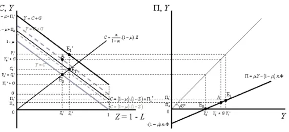
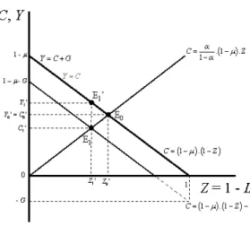
Figure 1: The Multiplier in the Dixon-Mankiw Model - Case I

in case I, where government can increase its consumption without rising taxes on households (dT₀ = 0). Consequently, we conclude that, in this case, a unit increase inGleads to an increase in equilibrium aggregate output of1=(1 : )>1. Further-more, note that this increase is larger than the one that would occur under perfect competition ( = 0 and = 0), where it would be equal to 1.

We can better explain what happens by using Figure 1 below.

First, consider that in the initial equilibrium government expenditure is zero (G= 0) and pro…ts are also zero ( = 0). On the left-hand panel we can depict the microeconomic decision in the leisure-consumption space using two simple graphical tools: the upward-sloping income-expansion path and the downward-sloping budget constraint. The former corresponds to equating the marginal rate of substitution between leisure and consumption (M RSZ;C UZ=UC = (1 ):C=[ :Z] in this

model) to the real net wage (!_N = 1 in this model). The later is just taken from equation (4), given the equilibrium values for the wages, pro…ts, and taxes.

Thus, the microeconomic equilibrium for the representative household is given by point E0 where it chooses an amount of leisure equal to Z0 and an amount of

budget constraint. Using the same amount of labour (leisure), the macroeconomic equilibrium is now given by point A. That increase in demand leads to an increase in pro…ts, as represented by point A in the right-hand panel. Thus, the microeco-nomic budget constraint would shift upwards and households would increase both leisure and consumption. But then, the macroeconomic constraint would also shift upwards, pro…ts would increase and so on until the process ends in a new equilibrium represented by points E1 (in both panels) and E1’ (in the left-hand panel).

In a nutshell: when …scal authorities stimulate aggregate demand through an increase in public consumption in the amount of one unit, there is an "initial" increase in output of the same amount (here, in case I). However, the mechanism does not stop there, as a larger aggregate income implies larger pro…ts that are distributed to households. Consequently, households initiate a new "round" of the mechanism as the increase consumption, in the amount of units, that will stimulate aggregate demand once more, that stimulates output...

However, for output to increase, it is necessary that private-sector employment (N) increases. Apparently, there is a contradiction with the graphical results as leisure also increases. Nonetheless, a larger level of public consumption implies a smaller level of unproductive public employment, as we can see in equation (10.I), given by = (T0 G)=(1 ) in this case whereT0 is …xed.

Thus, despite the fact that L, total employment, decreases due to the negative e¤ect of higher pro…ts, there is an employment transfer from the public sector to the private sector that more than o¤sets the decrease in L19 _{and leads to an increase in}

N.

Let us now we assume that government cannot increase its consumption without increasing taxes on households (dT₀ =dG), then we are in case II, where we conclude that

k_Aj_dT

0=dG =

1

1 : >0, (30.A2)

i.e. a unit increase in G induces an equilibrium output increase of 0 < 1 <

(1 )=(1 : )<1.

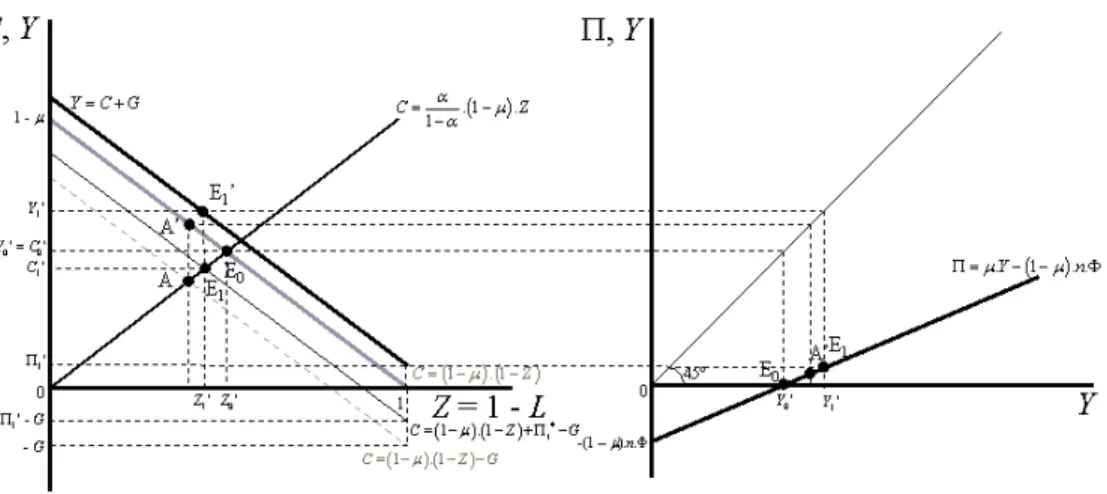
Figure 2 pictures the multiplier mechanism in a similar way to Figure 1. However, the initial demand stimulus is now also perceived by households as a tax increase, since

dT₀ = dG. Thus, the microeconomic budget constraint shifts down by the amount of lump-sum taxes (G). The negative income e¤ect moves the optimal decision of households from E0 to A, reducing both consumption and leisure. Nonetheless, the

macroeconomic Y = C+G curve does not move, and that means output increases

Figure 2: The Multiplier in the Dixon-Mankiw Model - Case II

to point A’. Consequently, pro…ts increase, as shown by point A’ in the right-hand panel, and another "round" of the multiplier mechanism is set in motion. At the end of the day, the new equilibrium is given by points E1 (in both panels) and E1’ (in the

right-hand panel).

In this case, the "initial" demand stimulus of one unit of government consumption is partially crowded out, leading to a output increase of 0 < 1 < 1 and then to a pro…ts increase of :(1 ), before the second "round" starts. Notice here the output increase can be easily explained by the labour-supply side: more government expenditure means more taxes and these have a positive e¤ect on labour supply that more than o¤sets the negative e¤ect of pro…ts20_{. Thus, households are willing to work}

longer hours as their disposable income decreases, the same reason that makes them consume less.

In both these cases (I and II) we observe that …scal policy e¤ectiveness on output is an increasing function of the degree of monopoly that exists in the economy:

@k_A @ _dT

0=0

=

(1 : )2 >0; @k_A

@ _dT 0=dG

= : 1

(1 : )2 >0. (31.A)

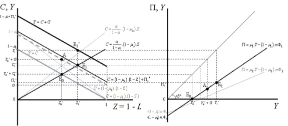
In order to explain what happens, let us use Figure 3 that refers to case I.

This …gure is very similar to Figure 1, but it assumes a larger mark-up level ( ₁ > ₀), i.e. a smaller elasticity of substitution amongst goods. In order to keep zero pro…ts in the initial equilibrium, we also assume a larger …xed cost ( 1 > 0).

As we can see in the left-hand-side panel, the larger mark-up level induces a smaller

Figure 3: The Multiplier and the Mark-up in the Dixon-Mankiw Model

equilibrium wage rate, inducing a downward rotation on the income expansion path around the origin and also a downward rotation of the budget constraint about point (1,0). On the right-hand side, a larger mark-up rotates the pro…t function up, but the larger …xed costs shifts it down in a parallel way.

Since the mechanism is similar to the one described in Figure 1, we can notice the output increase (Y₁ Y₀) is larger here than before, with a weaker monopoly power. So why does this happen? The answer lies on the combination of three e¤ects: i) there is a negative substitution e¤ect on labour supply due to the lower wage rate; ii) but the income e¤ect of the lower wage rate is positive; and iii) there is a negative e¤ect on labour supply due to larger pro…ts. Thus, the crucial e¤ect is the last one: a higher mark-up induces a larger pro…t windfall that will lead to a larger consumption by households, reinforcing the second-round e¤ect of the multiplier.

In case II, where there is no partial substitution of public employment by private employment, the mechanism of pro…t distribution is as important as here, but the e¤ect on labour supply is clear-cut: people would want to increase hours worked by more than in the case depicted in Figure 2. This is due to the reinforced negative e¤ect of taxes when the rate is lower.

imperfect competition, not in e¤ective demand scarcity. The e¤ect of …scal policy on welfare in case II, the only truly sustainable type of …scal policy in a static model, is clear: output increases by less than public consumption. Thus, private consumption decreases due to the e¤ect of higher taxes. Therefore, households work harder and their welfare decreases as a consequence of both e¤ects.

2.4.2 Taxation

One of the critiques to the works of Dixon (1987) and Mankiw (1988) is the fact that they use lump-sum taxes to …nance government expenditure. Molana and Moutos (1991) study the e¤ect of proportional taxes in balanced-budget model without un-productive labour. Thus, the basic assumptions we have here are = 0,T₀ = 0, and

0< t <1. All the other assumptions are identical to the previous point.

In what concerns to households, their behavioural functions are now given by

C = :(1 t):w+

P , (8.B)

L= 1 (1 ):(1 t): w+

w:(1 t). (9.B)

Given the static equilibrium sustainability issue in a framework with a minimum of consistency, from this point onwards we assume the government always follows a balanced-budget rule without recurring to unproductive labour. Here, considering there are no (net) autonomous taxes, we are in case III, i.e. we have dt = (1

k :g ):dG=Y to substitute in equation (30).

Thus, we obtain an equilibrium multiplier given by

k_Bj_{dt =(1 k :g ):dG=Y} = Y :(1 + )

B

, (30.B)

where B =Y :(1 + ) + :(1 g ):(1 + :Y ).21 At …rst sight,

the numerator, and also the denominator, appears to be either positive or negative. However, since we know thatC = (1 g ):Y and using equation (8.B) in addition, we have C = :(1 t ):(1 + ). If we also consider that the government budget constraint implies that t =g , it is simple to see thatY = :(1 + ). Therefore, k_Bj_{dt =(1 k :g ):dG=Y} = 0, i.e. …scal policy is absolutely ine¤ective in this case III22_.

21_{Since we know that, in equilibrium, we have (1 )< :Y = (1 ):n: <0, then}

we have B =Y :(1 + ) + :(1 g ):(1 ):(1 n: ). The constraintn: <1 is a

consequence of having1 L N n:m: 0.

22_{With the information obtained for the numerator, we know now that}

B =

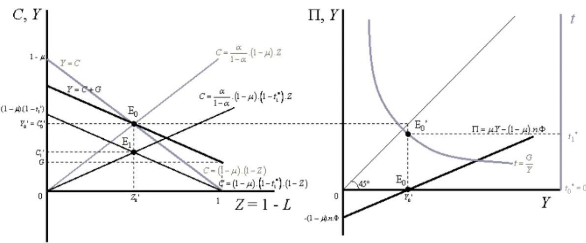
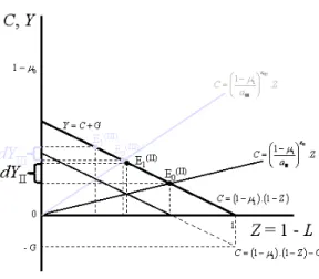
Figure 4: The Multiplier with Proportional Taxes

In Figure 4 we can observe what happens, starting from an initial equilibrium E0 with G = 0, t = 0, and = 0. On the left-hand-side panel we now have a

secondary axis to represent the tax rate, a decreasing function of output givenG >0. Thus, when positive government consumption is introduced, the tax rate increases from zero tot1 >0. This implies a downward rotation of both the income expansion

path and the budget constraint. In the new equilibrium E1, private consumption was

completely crowded out by government consumption and output, leisure, and pro…ts remain unchanged, given the functionals assumed.

So, why is there such a dramatic loss of e¤ectiveness? Contrary to case II, here an increase in public consumption only presents a potential substitution e¤ect on labour supply, as it implies a tax-rate increase. However, this tax-rate increase has identical consequences on pro…ts and wages, as they are both taxed at the same rate. Thus, the incentive to work more ceases to exist, unless pro…ts decrease. But to have a decrease in pro…ts, we would need an output fall and that is not compatible with an increase in employment in this case.

Molana and Moutos (1991) also demonstrate that, when taxes are levied only on wage income, we may even obtain a negative multiplier.

Considering there is no e¤ect on output, here where there are only distortionary taxes, private consumption decreases and leisure remains unchanged. Once again, households welfare is smaller after implementing the expansionary …scal policy.

2.4.3 Entry

Figure 5: The Free-entry Multiplier of Startz

Dixon (1987) and Mankiw (1988) models assume the economy is in a "short-run" situation, i.e. …rms are not allowed to enter or leave the productive sector. However, this situation is not sustainable in the "long run," an environment more suitable to be portrayed by a static model, corresponding to a steady state of a dynamic model. Startz (1989) presents a "long-run" model using the basic assumptions in both Dixon (1987) and Mankiw (1988)23_{. Thus, the basic assumption here is that the mass}

of industries (or varieties), n, is not a constant, but an endogenous variable resulting from a zero-pure-pro…ts condition. In our case, where there is no uncertainty or dynamics, since there is no opportunity cost of creating a new …rm (or shutting down and existing one), the condition mentioned can be written as = 0.

Therefore, non-wage income ceases to respond to …scal-policy impulses, as _G = 0. This feature cuts the transmission mechanism though pro…ts into consumption and from consumption to aggregate demand again. Then, the multiplier is given by

k_CjdT₀=dG

G=0

= 1 >0. (30.C)

This multiplier is still positive, in the(0;1)interval, but it does not depend on the existing monopoly-power level in the economy. Thus, in this model …scal policy e¤ec-tiveness would be identical in the Walrasian case ( = 0) and in a highly monopolised economy ( !1).

23_{In fact, Startz (1989) uses a Stone-Geary utility function instead of a Cobb-Douglas. However,}

Figure 5 shows us what is happening in the free-entry model. There is no need for the right-hand-side panel as pro…ts are compressed to zero by entry and exit. Thus, an increase in G shifts the microeconomic budget constraint down and the income e¤ect of higher taxes induce an increase in labour supply and a decrease in consumption. Therefore, aggregate output increases, but there is a partial crowding out of private consumption of units for each unit of government consumption.

We can also notice that a change in moves the income expansion path and the budget constraint, but it does not alter the result in terms of …scal policy e¤ectiveness as they both rotate in the same proportion like in the ‡at-rate-tax case.

Furthermore, we can observe the free-entry (or "long-run") multiplier, given by equation (30.C), is larger than the no-entry ("short-run") multiplier given by equation (30.A2):

A(C)

k_CjdT₀=dG

G=0

k_Aj_dT

0=dG

= 1 : <1.

As we saw when comparing both models with the same lump-sum tax …nancing public expenditure, the main di¤erence between these two types of model is the way pro…ts distribution a¤ects private consumption. Once this mechanism is shut down, only the income e¤ect in labour supply subsists to increase output, with the preferences assumed.

2.4.4 Preferences

The main result of Startz (1989) is extremely appealing, as it eliminates the multiplier pure-pro…t mechanism.

However, Dixon and Lawler (1996) demonstrate that conclusion is clearly depen-dent on the type of preferences assumed for households24_{. If we keep the assumptions}

in Startz (1989), what some authors call the Dixon-Mankiw-Startz (DMS) framework, with the exception of the Cobb-Douglas utility function, we can see the no-entry mul-tiplier is given by

k_D1j_dT

0=dG =

1 C

N

1 C

N:

>0, (30.D1)

which is positive and less than one if we assume the marginal propensity to consume of net non-wage income is restricted to the(0;1)interval, as in the particular case of the DMS framework whereC

N = .

Considering free entry, we obtain the "long-run" multiplier given by

24_{In fact, that article also demonstrates Startz’s result also depends upon the production}

k_D1jdT₀=dG

G=0

= 1 C

N >0, (30.D2)

which was constant and equal to 1 in Startz (1989) particular case.

Assuming u( ) still represents homothetic preferences, the graphical representa-tions are similar to Figures 2 and 5 and the only di¤erence is that the income ex-pansion path is now given by C = (1 ):Z, where ( ) is a general increasing function. If we assume preferences are not homothetic, the income expansion path becomes non-linear, but the outcomes are identical.

Furthermore, it is easy to observe the no-entry multiplier is larger than the free-entry one:

D1

k_D1jdT₀=dG

G=0

k_D1j_dT

0=dG

= 1 C

N: <1,

and this result is also easily explained by the neutralisation of the pro…t e¤ect25_.

Thus, the previous results are similar to the DMS framework and we only have to substitute by C

N. However, in general, the marginal propensity to consume of

pro…ts depends upon the mark-up. Therefore, the "long-run" …scal multiplier is the larger (smaller) the larger is the market power in the economy, whenC

N is decreasing

(increasing) with .

Let us study an example using the utility function in Heijdra and van der Ploeg (1996)26_{, i.e. CES preferences over the consumption basket and leisure:}

U = C" 1 +a:Z" 1

" " 1

, (1.D2)

In this case, the private consumption function is given by

C = :w+ T0

1 +a"_:w1 ", (8.D2)

from which we can easily observe the marginal propensity to consume previously referred is not constant, but it is an endogenous variable that depends on the equilib-rium value of the real wage rate: C

N = (1 +a

"_:w1 "₎ 1_{. Notice also that (1 ) =} [(1 )=a]" in this case.

Considering that we have w = 1 , this marginal propensity is decreasing (in-creasing) with the mark-up when the elasticity of substitution between consumption and leisure (") is less (more) than one. Thus, …scal policy is more (less) e¤ective the

25_{Dixon and Lawler (1996) also demonstrate this is not always the case when production}

technol-ogy does not exhibit constant marginal returns.

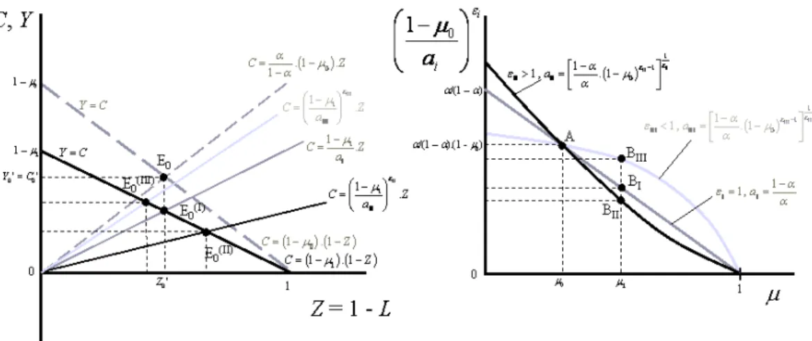
Figure 6: The Mark-up and the Equilibrium with CES Preferences

more imperfect competition is in this economy. However, di¤erent preferences may lead to di¤erent results.

We can see what happens using Figure 6. Consider an initial mark-up given by

0 and three sets of parameters:

- In set I we have "I = 1and aI = 1 . This corresponds to the case analysed in

Startz (1989).

- In set II we have "II >1 and aII = 1 :(1 0) "II 1

1 "II_.

- In set III we have "III <1 and aIII = 1 :(1 0) "III 1

1 "III_.

Notice that we have i(1 0) = (1 )= for all i = I; II; III. Thus, the

graphical representation of the initial equilibrium with = ₀ is the same for the three cases and it would also be the same after using …scal policy (see Figure 5). However, for ₁ = ₀ there is a di¤erence: the income expansion path rotates at di¤erent rates.

We can see what happens to the functions i(1 )on the right-hand-side panel.

For a unit elasticity of substitution, as in the Cobb-Douglas case, this function is linear in . However, it becomes concave (convex) for values of"smaller (greater) than one. This, the substitution e¤ect of …scal policy will be quite di¤erent in these three cases, when the mark-up varies.

Figure 7 presents the output multiplier for cases II and III.

Figure 7: The Mark-up and the Multiplier with CES Preferences

path, when compared to the initial situation. In case II, a larger mark-up means a larger substitution e¤ect. Thus, considering the e¤ect on the budget constraint is the same in both cases, an increase in government consumption induces a higher increase in labour supply in case II than in case III. A larger elasticity of substitution means that households are willing to accept a higher reduction in leisure (and a smaller decrease in consumption) in order to respond to the corresponding tax increase.

2.4.5 Increasing returns to variety

Let us now return to the functionals assumed in the DMS framework. However, we assume there is some taste for variety, i.e. > 0. In this case, equation (25) tell us that, for a given mark-up level, the real wage is an increasing function of the mass of goods existing in the economy.

This type of models, considering the love-for-variety assumption, is treated in Heijdra and van der Ploeg (1996)27_{. For sake of simplicity, we treat these two e¤ects}

separately. Devereux et al. (1996) present a dynamic model where a similar e¤ect arises from increase returns to specialisation, a kind of love for (intermediate-inputs) variety in the production function.

When the mass of …rms and goods (n) is …xed, i.e. when there is no entry or exit, the …scal multiplier is still given by equation (30.A2). However, if …rms are free to enter or leave the market, their mass becomes an endogenous variable given by

n =h₍₁ :Y_): i1 ; = _{+ 1} 2[0; ], (32)

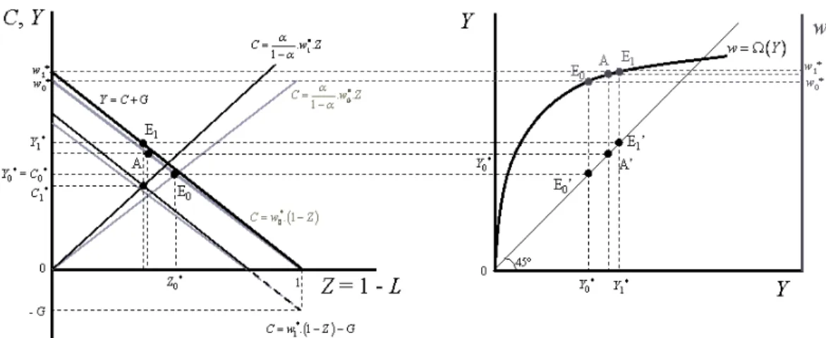
Figure 8: The Multiplier with a Varying Real Wage

a result that is obtained through the free-entry condition = 0.

Thus, an aggregate demand increase induces an increase in real wages that will a¤ect …scal policy e¤ectiveness as28

wG = :

w

Y :k = :[1 (1 ):g ]:k > 0,

i.e. entry of …rms, a consequence of the aggregate demand stimulus, leads to a real wage increase and consequently to a consumption increase, opening a transmission channel similar to the pro…t one in the no-entry model. In this case, the multiplier is given by

k_EjdT₀=dG

G=0

= 1

1 :[1 (1 ):g ] 0. (30.E)

Notice that, due to >0we have >0and consequently a larger multiplier than in the free-entry constant-returns case (1 ).

On the left-hand-side panel of Figure 8 we can observe that …scal policy would change the equilibrium from point E0 to point A. That is the situation depicted in

Figure 5, corresponding to a …xed-wage environment. However, point A is not an equilibrium in this model, as the real wage is a function of the aggregate outputw = (Y) with 0_{( )>0. This fact can easily be observed by combining equations (25)}

and (32). Therefore, a higher output induce new …rms to enter and that stimulates

aggregate demand via private consumption in the case of love for variety and labour demand in the case of increasing returns to specialisation. In any case, the equilibrium wage rate goes up, as we can observe on the secondary axes of the right-hand-side panel of Figure 8. The wage increase rotates the income expansion path, the household budget constraint, and the macroeconomic constraint up in the left-hand-side panel. The new equilibrium is …nally reached in point E1with a larger output and a smaller

decrease in private consumption.

Despite the fact that we are using a consumption function with constant marginal propensities to consume, this multiplier depends upon the monopoly power level in the economy throughg and = : =( : + 1 ). It is simple to demonstrate that is increasing with the mark-up29_{, but it is not easy so show how does g depends}

on . A …rst glance, one could think the weight of public consumption in output should be increasing with the monopoly degree, as it means more ine¢ciency, thus less output. However, taking into account net pro…ts are zero, the macroeconomic production function can be represented as

Y = (1 ):n 1:L.

In the equation above we can observe that, for the same employment level, an increase in leads to a reduction in the term (1 ), but it also increases the exponent, as it corresponds to a reduction in . This means that the monopoly degree under monopolistic competition reinforces the e¤ect of increasing returns. There is also an indirect e¤ect that acts throughn, since an increase in stimulates entry.

Therefore, we can easily determine what is the e¤ect on the multiplier when we start from a zero-government-consumption steady state

@k_E

@ dT0=dG G=0

g =0

= 1

(1 )2:[1 :(1 )]2 0.

In this particular case, the larger is the market power, the larger is the entry e¤ect on the real wage, increasing the e¤ectiveness of the initial …scal stimulus. An identical outcome can be obtained for situations whereg does not react dramatically to changes in the mark-up. Using numerical simulations with plausible values for the parameters, we also obtain a multiplier that is an increasing function of .

Now comparing the "short-" and "long-run" multipliers, we observe that

E

k_EjdT₀=dG

G=0

k_Aj_dT

0=dG

= 1 :

1 :[1 (1 ):g ].

29@

@ =

2

Considering that and g depends upon the values of other parameters in the model, it is not possible to say a priori if this value is larger of smaller than one. Thus, we know that for < :[1 (1 ):g ] the free-entry ("long-run") multiplier is larger than the multiplier with a …xed mass of …rms, given the positive externality caused by the entry of new …rms. The opposite result is obtained when the mark-up is high.

2.4.6 Endogenous mark-ups

The assumption that entry of …rms is done through the creation of new monopolies associated to new products hides an additional assumption that product innovation is cheaper than copying an existing good or creating a close substitute. When facing signi…cant costs associated with creating a di¤erentiated product, the incentive to create a new industry may be smaller than the incentive to enter an existing industry. Thus,m may be the endogenous variable in our free-entry model instead ofn.30

Up to this point, we considered that was an exogenous variable, as we assumed

m was …xed and equal to one (a basic assumption in monopolistically competitive models). When we alter the endogenous variable in the entry process, we also endo-genise = 1=( :m). This value can be obtained through the zero-pro…t condition, assuming once again there is no love for variety ( = 0):

=

1 + , (33)

where = n: =Y is an increasing returns to scale indicator for the production function and it represents the weight of total …xed costs in aggregate output. We can notice its equilibrium value is a decreasing function of the equilibrium output. Note that, in this case, the market power has a negative correlation with aggregate output, which is consistent with counter-cyclical mark-ups as documented in the empirical literature31_.

Despite the fact this hypothesis is considered in Dixon and Lawler (1996), the treatment of …scal-policy e¤ectiveness in an endogenous-mark-up framework is done in Costa (2004). However, there are other endogenous-mark-ups models, though not speci…cally dedicated to …scal-policy e¤ectiveness, that are surveyed in Rotemberg and Woodford (1999).

In the case treated here, it is the real wage that reacts to …scal policy, as we have

w = 1 . Nonetheless, considering the reduced-form macroeconomic production function with free entry Y = (1 ):L, the endogenous mark-up may work as a

30_{For a more detailed analysis of the underlying process and its fundamentals see Costa and Dixon}

(2007).

productivity shock, but it originates in the aggregate-demand side in the case of …scal policy32_.

Thus, an increase in public consumption translates into a mark-up reduction, i.e. a real-wage increase w_G = ( )2:k =(n: ) > 0. Therefore, the increase in intra-industrial competition induced by an expansionary …scal policy leads to an second stimulus in private consumption, via real wages, reinforcing the multiplier mechanism and acting as a positive externality:

k_FjdT₀=dG

G=0

= 1

1 (_n:)2 0. (30.F)

The graphical representation of this mechanism is also given by Figure 8, where

w = (Y) is obtained from equation (33). Despite the di¤erence in the economic mechanism, the real-wage transmission mechanism is similar to the previous model.

Considering that is now an endogenous variable, it makes no sense to calculate the derivative of this multiplier in order to the mark-up. However, any change in the parameter values or exogenous variables that leads to a higher mark-up (e.g. a smaller public consumption or a higher …xed cost) induces an increase in …scal policy e¤ectiveness.

Finally, considering the no-entry mechanism is the same as in the previous case, we have

F

k_FjdT₀=dG

G=0

k_Aj_dT

0=dG

= 1 : 1 (_n:)2.

Thus, near the initial equilibrium where = , the "long-run" multiplier is larger than the "short-run" one, as long as the monopoly power indicator is su¢ciently large, i.e. as long as > :n: .

Molana and Zhang (2001) study the steady-state e¤ects in an intertemporal model similar to Costa (2004), where they assume that = (n) with 0_{(n)<0. In a way}

similar to Galí (1995), these authors assume that there is imperfect competition in intermediate goods markets used to produce …nal goods and where a larger mass of varieties increases the elasticity of substitution amongst them. Despite the di¤erent endogenous mark-up generation mechanism, the qualitative results are similar33_.

In both the endogenous mark-up and the taste for variety (or increasing returns to specialisation) cases, …scal policy (or aggregate demand management policy in

32_{There is an recent interest in this subject in the business-cycle literature. For an example, see}

Barro and Tenreyro (2006),inter alia.

33_{Chen et al. (2005) present a model that intends to extend the DMS framework to an}

general) have a positive e¤ect on the e¢ciency level in the economy. This allows the balanced-budget multiplier to be greater than one and simultaneously, for a given employment level, the output to be larger. Consequently, taking into account the multiplier e¤ect of public over private consumption is given byk 1, it is possible to obtain a positive …nal e¤ect on households consumption. For the same reason, leisure will not decrease so much as in the previous cases.

Therefore, it is possible that …scal policy, without any direct externalities, has a positive e¤ect on households welfare as long as: i) the e¤ect of the e¢ciency gain is large enough to guarantee that k >1and ii) the increase in private consumption is su¢ciently important to o¤set the reduction in leisure.

2.4.7 Extensions and generalisations

Many additional works try to analyse the relationship between market power and …scal policy e¤ectiveness, but we cannot go through all of them here. However, some of the most interesting results can be brie‡y described in this section.

Amongst static models, Molana and Montagna (2000) introduce heterogeneity in the marginal product of labour in a DMS-style framework, also keeping love for vari-ety. There, the zero-pro…t condition only applies to the "marginal …rm (industry)," the reason why its more e¢cient competitors present positive pro…ts. In their model, the absence of taste for variety leads to the entry of less e¢cient …rms, so it reduces the average e¢ciency of the economy and also …scal policy e¤ectiveness. Love for variety tends to oppose this e¤ect.

Still considering static models, Torregrosa (1998) supplies a demonstration for the conjecture in Molana and Moutos (1991) stating that a negative multiplier can be obtained when there exist only proportional taxes on labour income. Reinhorn (1998) studies optimal …scal policy in a framework where public consumption directly a¤ects consumers utility.

Finally, Censolo and Colombo (2008) study the way …scal policy e¤ectiveness is in‡uenced by di¤erences between the composition of private and public expenditures, when di¤erent market structures (perfect and monopolistic competition) exist simul-taneously in the same economy.

3

Intertemporal models

section34_.

3.1

Intertemporal household

In particular, the instantaneous household utility follows as before: 1 and 2 with

= 0:The in…nitely-lived household has a discount rate of >0and, instead of (1), it maximises lifetime utility:

max C;Z U =

Z 1

0

u[(C( ); Z( )]:e : :d . (34)

In the dynamic model the household owns capital K( ) at moment which it rents out to …rms at pricer( ): hence its total income at timet is as before, labour income

w( ):L( ) and equity pro…ts ( ), plus the income from capitalR( ):K( ).35

Notice that, with an in…nitely-living household, Ricardian equivalence holds. Thus, since we are not interested in studying how public debt evolves overtime, noth-ing is lost if we assume government follows a balanced-budget rule at each moment . Also, for simplicity in this section we will assume that the government …nances expenditure by a lump-sum tax P ( ):G( ) = T0( ), i.e. we have ( ) = 0 and

t( ) = 0.

We still consider the preferences for varieties given by equation (2) and the re-source constraint in equation (3). Therefore, the intertemporal budget constraint can be simply expressed in terms of aggregate variables. The household can choose to allocate its income between consumption, paying tax or accumulating capital. The accumulation of capital is thus:

_

K( ) = w( ):L( ) +R( ):K( ) + ( )

P ( ) C( ) G( ). (35)

For simplicity we ignore time indices ( ) from this point onwards. Also, we continue to choose the composite good as numéraire, soP ( ) = 1.

3.2

Firm and production

The representative …rm’s decision is inherently static, since it rents capital from the household. Each instant , the …rm employs labour and capital to produce output:

yi(j)= max F(Ki(j); Ni(j)) . (36)

34_{This model is based on lecture notes by Huw Dixon "Imperfect competition and}

macroeco-nomics" used for PhD courses given at a variety of institutions, including Finnish Doctoral Pro-gramme 1996, ISEG/TULisbon 1999, Munich (CES ifo) 2000, as well as York and Cardi¤.

35_{We ignore depreciation of capital in order to keep the presentation simple. Considering a positive}

where we assume that FK > 0, FN > 0, FKK < 0, FN N < 0, FKN > 0, also that

functionF ( )is homogeneous to degree 1 (HoD1), i.e. the technology would present constant returns to scale (CRtS) if was equal to zero, and the Inada conditions hold. The …rm faces the demand curve (16). Given the real wage and rental on capital, the …rst order conditions for pro…t maximization imply (in a symmetric industry equilibrium):

(1 ):FKi(j) =R; (1 ):FN i(j) =w. (37)

Since the marginal products of labour and capital are the same across all …rms (this is ensured by competitive factor markets), we can rewrite the household’s accumulation equation using (37) as

_

K = (1 ):(FN:N +FK:K) + C G.

Since function F( ) HoD1 in(K; N), by Euler’s Theorem36 _{we have:}

_

K = (1 ):F(K; N) + C+G.

Furthermore, in a symmetric equilibrium where p(j) = P = 1, the pro…ts of each …rm are simply:

i(j) = p(j):yi(j) T Ci(j) = = yi(j) w:Ni(j) R:Ki(j) =

= F(Ki(j); Ni(j)) (1 ):F Ki(j); Ni(j) = = :F Ki(j); Ni(j) ,

so that aggregating across all …rms we have

= :F (K; N) n:m: . (38)

whereN =R₀n X i(j)2=(j)

Ni(j):djis the total demand for labour andK = Rn

0 X

i(j)2=(j)

Ki(j):dj

represents total demand for capital. Again, equilibrium in the labour market implies that N =L.

Under imperfect competition, a wedge is driven between the marginal product of each factor and the factor return: this leads to each additional unit of output yielding a marginal pro…t of (since only a proportion (1 ) is used to pay for labour and capital. There is also the overhead …xed cost, which may make the pro…t per …rm negative or positive, depending upon the level of output.

36_{WhenF( )is HoD1,F(K; N) =F}

3.3

The household’s intertemporal optimization

The household chooses (C( ); L( )) to maximize lifetime utility (34) subject to the accumulation equation (35), in e¤ect a dynamic budget constraint. The current-value Hamiltonian for this intertemporal optimisation problem is

H=u(C;1 L) + :(w:L+R:K + C G),

The …rst-order conditions for this are

HC uC = 0;

HL uZ+ :w = 0;

HK :R= _ + : ;

lim

!1 e

: _{: ( ):K( ) = 0.}

Using (37) we can express (w; R) in terms of the marginal products. Hence, we derive two basic optimality conditions:

Intra-temporal optimality Once again37_{,M(C; Z);the marginal rate of}

substitu-tion between consumpsubstitu-tion and leisure equals the net real wage rate

M(C; Z) uZ

uC

= (1 ):FN.

Inter-temporal optimality The Euler condition. Assuming that uCZ = 0, i.e.

assuming the felicity function is additively separable, this can be written as

_

C

C = :[(1 ):FK ],

where uC=(C:uCC) is the elasticity of intertemporal substitution in

consump-tion.

3.4

Steady State

In the steady state, we have the condition that C_ = 0: Hence the Euler condition implies that

(1 ):F_K = ,

where asterisks stand for steady-state values. In the Walrasian case ( = 0) this is just the modi…ed golden rule. What imperfect competition does is to discourage

investment, since the returns on investment are depressed (there is a wedge between the marginal product and the rental on capital.

Now, under the assumption that functionF ( )is HoD1, we can write it in factor intensive form F(K; L) = L:F K_L;1 =L:f(k), where k K=L. Hence the steady-state Euler condition is

f0_{(k ) =}

1 , (39)

where f0_{(k) =F}

K K_L;1 >0 and f00(k) =FKK K_L;1 <0.

Let us now consider the special case of monopolistic competition where every industry is a monopoly, i.e. m( ) = 1. In this case, given the CES preferences in (2), the mark-up is also constant and given by ( ) = = 1= .

With this particular market structure we can write the solution to this as k =

k ( ) with k 0 _{< 0. With F( ) HoD1, the steady-state Euler condition is very}

powerful: not only is the marginal product of capital determined, but so is the steady-state wage rate

w ( ) =f[k ( )] :k ( )

1 . (40)

With this we have the income expansion path (IEP) for consumption and leisure, de…ned by the intertemporal optimality condition and the steady state wage

u_Z

u_C = (1 ):FN =w ( ). (41)

As in the static model, the IEP will be upward sloping in (Z; C), since both con-sumption and leisure are normal; it will be linear if preferences are quasi-homothetic; it will be a linear ray through the origin if preferences are homothetic.

There is a steady-state relationship between income and consumption given by38_:

C =L :f[k ( )] n : G . (42)

We will call this the Euler frontier (EF).

38_{This can be derived from the budget constraint:}

C = w ( ):L +R :K + G =

= w ( ):L +

1 L:k ( ) + :L :f(k ) n : G =

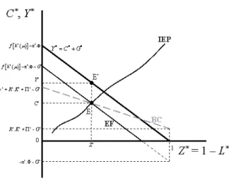
Figure 9: The Steady-State Equilibrium

Note that the EF is not the household’s budget constraint (BC). Let us take the case of where the number of …rms is …xed. The household receives pro…t income , which it sees as a lump-sum payment, and also the rental income on capital. The household thus only sees the variation in labour income as it considers varying L : the slope of the actual budget constrain is thusw ( ). The actual budget constraint is given by the grey dotted line in Figure 9: if the household is at point E0, it is ‡atter

than the EF. Also, at the intercept there is all of the non-labour income (rental on capital, pro…ts less tax).

The unique steady-state equilibrium is the found at the intersection of the IEP and EF at point E0, as depicted in the same …gure39. Here we can see the equilibrium

level ofC andL = 1 Z . The optimal capital stock is then simplyK =L :k ( ).

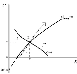
3.4.1 Dynamics

Whilst the steady state is best understood in terms of leisure-consumption space, the dynamics is best understood in the classic Ramsey projection(K; C). As a …rst step, we need to note that the intratemporal relationship means that we can de…ne labour supply as an implicit function of (C; K) : L = L(C; K; ); with LC < 0 < LK and

L <0.40

39_{Uniqueness is not guaranteed when we have a signi¢cant taste for variety, i.e. is large, when}

the mark-up is endogenous, i.e. = (k ), or when there are increasing returns to scale at the aggregate level.

Figure 10: The Saddle-Point Stable Equilibrium

The dynamics are represented by the two isoclines:

_

C = 0 : (1 ):FK[K; L(C; K; )] = 0; (43) _

K = 0 :F [K; L(C; K; )] n: G C = 0. (44)

The consumption isocline isdownward sloping in(K; C): it is de…ned by the equality of the marginal revenue product of capital being equal to the discount rate. To the right of the consumption isocline, consumption is falling, since(1 ):FK < ; to the

left it is increasing. The capital isocline has the standard upward-sloping shape41_{: it}

need not be globally concave due to the e¤ect ofK on the labour supply. The phase diagram thus has a unique saddle-path solution as depicted in Figure 10.

3.5

The e¤ect of imperfect competition on the long-run

equi-librium

In this section we illustrate the e¤ect of a change in on the steady-state equilibrium from both (1 L; C) space and (K; C) space. First, let us analyse the consequences of imperfect competition in leisure-consumption space. We have two e¤ects of an increase in the degree of imperfect competition:

41_{See appendix 7. Notice that with >0the capital isocline would present the usual hump shape:}

Figure 11: Market Power and the Steady-State Equilibrium (I)

The EF curve rotates anti-clockwise. Since we have

f0(k ) =

1 ;

dk

d =

f0_{(k )}

(1 ):f00_{(k )} = _{(1 )}2_:f00_{(k )} <0.

The real wage falls, so that the IEP moves to the right. Since from (40)

w ( ) = f[k ( )] :k ( )

1 ;

dw

d =

:k ( ) (1 )2 <0.

These two e¤ects are depicted in Figure 11, where the equilibrium moves from E0

to E1 when we compare a low-markup steady-state ( = 0) with a large-markup one

( = 1 > 0).

Figure 12: Market Power and the Steady-State Equilibrium (II)

Turning to capital-consumption space and the phase diagram, the way to under-stand the e¤ect of is via the e¤ect onL: for given(K; C), an increase in increases the wedge between the marginal product of labour and the wage, hence leading to a reduction in the labour supply. Less labour means that both total output and the marginal product of capital fall. Hence we have two e¤ects of an increase in :

The consumption isocline shifts to the left (sinceFK falls asL decreases).

The capital isocline shifts downwards, as there is less output given(K; C).

The shift from equilibrium E0 to E1 in Figure 11 is represented in(K; C)in Figure

12. Note that whilst steady-state consumption falls, the e¤ect on capital is potentially ambiguous. This is because the e¤ect of on labour supply is ambiguous. Here capital decreases, which is compatible with the reduction in employment observed in Figure 11.

3.6

Free Entry

Until now, we have assumed that the number of …rms is …xed across time, so that

n( ) =n. In this case, aggregate output is given by:

Y( ) =L( ):f[k( )] n: . (45)

If there is instantaneous free entry which drives pro…ts to zero, from (38), for given

(K; L);pro…ts are zero when