Predicting Amazon Deforestation through the deterninants of demand for agricultural land

F U N D A

ç

Ã

O

"

#"

Getulio Vargas

IPGI

Escola de Pós-Graduação em Economia

Seminários de Pesquisa Econômica I (2

parte)

"PBEDICTIl\TG AlVIAZOl\T

DEFOBESTATIOl\T TRBOUGR TRE

DETEBNal\T~SOFDEMAND

FOB AGBICULTUBAL LAl\TD"

L

YKKE

E.

ANDERSEN

/

,I!

(Univ. of Aarhus, Denmark)

..

..

----~---

-Predicting Alnazon Deforestation through the

Deterlninants of Delnand for Agricultural Land

Lykke E. Andersen*

Department of Economics

University of Aarhus, Denmark

E-mail: [email protected]

Eustáquio J. Reis

Institute for Applied Economics Research

Rio de Janeiro, Brazil

April 18, 1996 (Preliminary draft)

Abstract

This paper develops a model of deforestation pressure in the Amazon. It

is based on the determinants of demand for agricultural land, i.e. the interactions between population dynamics, urbanization and the growth of local markets, land prices, and government spending and policies. The mo deI is estimated using data from the period 1970 - 1985, and predictions for the period 1985 - 2010 are made under explicit assumptions about the underlying factors of deforestation.

The predictions indicate that economic growth in the Amazon is likely to continue at high rates even if the federal government abandons its ag-gressive development policy. Deforestation will be much smaller if they do, though, since the active development policies tend to promote wasteful use of land.

JEL classification: C53, Q23, Q28

Keywords: Tropical deforestation, simulation model.

* This research was carried out while the first author was visiting the Institute for Applied Economics Research in Rio de Janeiro and the hospitality of institute is gratefully acknowledged.

..

•

1. Introd uction

Many deforestation studies from the late eighties showed alarming predictions for the future speed of forest clearing in the Amazon. Applying an assumption of a constant annual percentage increase in deforested land, they fitted expo-nential trends to the available data, and with the few data points available this

assumption seemed to fit the data well up to 1988.

The assumption of an an exponential trend is very strong, as can be illustrated by the following example. According to data from the Brazilian Institute of

Statistics and Geography

(IBGE),

Legal Amazonia was about 3.9

%

extension of that trend would imply that the whole area of 5 million square

kilometers would be cleared by the year 2037. For some Amazonian states the

speed of clearing was much higher than that. Rondônia, for example, experienced

average clearing rates of 8.7 % per year during the same period. If that were to

continue the whole state would be cleared by the year 2015.

The latest deforestation estimates indicate that these trend projections were too pessimistic. The assumption of an exponential trend is also theoretically questionable, since it requires that the underlying factors of deforestation also grow at an exponential rate. While this may be reasonable for factors like output growth and population growth, it is hard to justify for factors such as road build-ing and govemment subsidies which are funded from a limited public expenditure budget.

The problem with trend projections is not only the assumptions of constant clearing rates, but also the assumption that the underlying factors of deforesta-tion remain largely unchanged during the projecdeforesta-tion period. A change in public priorities in the late eighties has indeed changed the trends of many of the

under-lying factors of land clearing (see, for example, Schneider 1992). As land becomes

more scarce a natural process of technical progress and substitution towards more labor-intensive and less land-intensive production methods will aIs o work against the exponential trend.

This paper develops a model of deforestation pressure in the Amazon. It is

based on the determinants of future demand for agricultural land, i.e. the in-teractions between population dynamics, urbanization and the growth of local markets, govemment spending and policies, and land prices. The mo deI is

in-spired by the theoretical model of Deacon (1995), but adapted to the data set

available in order to construct an empirically estimable model.

The model i8 estimated using data from the period 1970 - 1985.

Predic-tions for the period 1985 - 2010 are made under explicit assumptions about the

underlying factors of deforestation.

1 Clearing here means conversion of natural vegetation to agriculturalland uses (crops,

...

2. The model

Previous empirical work on the determinants of Amazon deforestation indicate that the main source of deforestation is conversion of forest to agriculturalland

(e.g. Andersen et al 1996, Reis and Guzman 1994, Brown and Pearce 1994).

Logging, fuelwood collection, mining, and infrastructure building, on the other hand, play only a minor role.

Since forested land in the Amazon has been virtually free for anyone who wanted to develop it, forest conversion is mainly determined by demand for agri-cultural land. The current mo deI is therefore constructed under the assumption that the main source of deforestation is the use of land for agropastoral activities. The demand for agricultural land on a particular location depends on the expected profitability of forest conversion. Profitability, in turn, is determined by factors such as accessibility, availability, market conditions, and fiscal incentives. The model consists of one ma in equation predicting the demand for cleared

land in region i at time t on the basis of past characteristics of region i and its

closest neighbors. In addition, there are 5 equations which explain the interaction between rural and urban populations, rural and urban output, and land prices. 2.1. Demand for agricultural land

Before 1960 there was very little economic incentive to create agricultural es-tablishments in the Amazon. Most of the region was virtually inaccessible, the soils were covered by dense and stubborn forest that would have to be removed before the land could be used, there were no local markets for neither inputs nor outputs, and there was a totallack of social infrastructure.

This changed, however, when the Brazilian government through ambitious road building and settlement programs decided to open up the region, and "bring men without land to the land without people." During the subsequent decades more than 10 million people suddenly found it economically sensible to settle down in the Amazon.

The settlement was not evenly distributed over the region, though. The east-ern and southeast-ern regions received far more migrants than the westeast-ern and north-ern regions, and clearing was visibly concentrated along the major highways, their feeder roads, and the big rivers, thus giving evidence to the criticaI importance of accessibility. In our empirical model accessibility of a region will be proxied by i) distance to the federal capital, Brasília, ii) extension of the road network, iii) length of main rivers in region, and iv) the leveI of clearing in neighboring municipalities .

As population densities increased in these areas and land became more scarce land prices were pushed up. This would naturally reduce the demand in areas where land was scarce compared to areas where it was abundant. To capture the efIect of land availability in our empirical model we use the following three

variables: i) rural population density, ii) land pnces, and iii) lagged leveI of clearing.

Besides the fundamental requirements of accessibility and availability of land, demand is affected by the economic prospects in a region. Because of the long distances and the high costs of transporting agricultural goods, farmers in the Amazon depend heavily on the availability of local markets. The economic viabil-ity of Amazonian agriculture has indeed depended critically on the rapid growth of urban markets that took place during the last decades (Schneider, 1992, p.12). The number of urban residents per rural resident in Legal Amazonia increased steadily from 0.6 in 1970 to 1.2 in 1991, and urban output grew at an impressive

rate of 7.7

%

is by far the dominant industry in the Amazon. This constitutes government, commerce, financiaI, and other services required to sustain the basic activities of agricultural, agro-processing, timber, and mining sectors (Schneider, 1992, p.12). The variables used to capture the local market conditions are the following: i) growth of urban output in region, ii) road length in region, and iii) distance to the state capital.

Other factors directly related to the profitability of agricultural settlement are land prices and fiscal subsidies and incentives. Agriculture in the Amazon has been an attractive tax shelter because of the virtual exemption from income taxation (Binswanger 1989, p. 20). This exemption naturally adds to demand for agricultural land, but it does so evenly over the whole region, and we are unable to measure the effect in our empirical model. However, some regions were

officially designated as growth poles, and enjoyed extra favorable conditions2.

We include a dummy for these regions to capture non-monetary incentives. The

distribution of monetary incentives is proxied by the amount of FINAM credit

obtained in each region in 1985.

For a potential migrant the leveI of rural income per rural capita in the pre-vious period is a good indicator for his expected future income. Relatively high expected income in a region will add to demand for land in that region so this variable is also included in our model.

The considerations above leads us to assume the following function for the demand for cleared land in Amazonia:

C LR_LAN Df; -

f

river lengthi, leveI of clearing in neighboring regionSi,t_l

speed of clearing in neighboring regionSi,t,

rural population densitYi,t-b leveI of clearingi,t_b

growth of urban outputi,t, distance to state capitali,

2For example the Free-zone of Manaus. For a full list and descriptions of the growth poles in Legal Amazonia, see Andersen et al (1996).

growth pole dUmmYi, FINAM _crediti,

land priceSi,t-I, rural in come per rural capitai,t-l, municipality areai)

Municipality are a is included to control for differences in municipality sizes, since big municipalities would tend to have more forest available for clearing.

For estimation purposes, we assume that the function is log-linear in the relevant space. To eliminate problems of causality, alI explanatory variables are

lagged so that stock variables are from time t - 1 while flow variables are from

the period between time t - 1 and time t.

2.2. Population dynamics

Total population in Legal Amazonia grew at an average annual rate of 4.0 %

during the period 1970 - 1991. The urban part of the population expanded much faster than the rural, though, leading to a dramatic change in the composition of the population. Since rural and urban persons have very different effects on deforestation, it is important to model these to groups separately. Urban persons typicalIy work in the service sector and is therefore assumed to have no direct impact on deforestation. There will, nevertheless, be an indirect effect through the demand for agricultural goods.

2.2.1. Rural population

The size of the rural population is determined partly by the size of the inherent population and partly by new immigration. The number of immigrants depends both on push and pulI factors. Push factors are population pressure in neigh-boring areas, while the main pulI factor is economic possibilities in the region. The economic attractiveness of a region depends on its accessibility, productivity, market conditions, and fiscal subsidies.

The size of the rural population in region i at time t can then be predicted

by estimating the folIowing function:

PO P _RU RALi _, t

f

neighboring regionSi,t-l, distance to federal capitali,

road lengthi,t_I, river lengthi, rural income per rural capitai,t-l, leveI of urban outputi,t-l, growth of urban outputi,t,

urban output per urban capitai,t-l, distance to state capitali,

growth pole dummYi, FINAM crediti, municipalityareai)

For estimation purposes it is again assumed that the function is log-linear in the relevant space.

•

2.2.2. Urban population

The size of the urban population is aIs o partly determined by the inherent urban population and partly by immigration. A relatively high urban income per urban capita is expected to attract people to the city, both when compared to rural incomes and when compared to urban incomes in other regions.

Other pull factors are fiscal incentives and a good urban infrastructure. As an indicator of urban infrastructure we use a composite variable which is the sum of the share of households which have running water, the share of households which have electricity, and the share of households which have sanitary installations.

Thus, we expect to be able to estimate the size of the urban population in

region i at time t from a function of the following form:

POP_URBANi,t = !(POP_URBANi,t-b urban income per urban personi,t-l

rural income per rural capitai,t-l, change in road lengthi,t_l, road lengthi,t-l, road length change in neighboring areaSi,t,

growth pole dummYi, FINAM _{crediti, urban infrastructurei,t_b}

municipalityareai). 2.3. Rural and urban output

Since the deforestation effects of urban activities are very different from those of rural activities, it is important to model the two sectors separately.

Agriculture's share of total regional output has fallen steadily from 30 % in 1970 to only 17 % in 1985. This trend alone has a dampening effect on deforesta-tion since we have assumed that only agropastoral activities have any significant effect on deforestation. In 1985 the overall composition of urban output was: industry (43%), financiaI sector (20%), commerce (12%), public administration (10%), transport sector (5%), and other services (10%).

An unusually large part of the urban sector is public administration, which is mainly funded by federal transfers. While the average share of public admin-istration in Brazil was about 5% of GDP, it was as high as 21 % in Acre, 17% in Roraima, 16% in Rondonia, and 13% in Amapa in 1985. In earlier periods those shares were even higher. For the new states in the Amazon, the big public sector represents an injection of demand into the local economy rather than a drain on local directly productive resources (Schneider 1992, p.13).

The leveI of urban output at time t in region i can be estimated on the

basis of the urban population size and its average productivity at time t - 1,

infrastructure conditions, the amount of fiscal subsidies, and the quality of the urban infrastructure.

road lengthi,t-l, change in road lengthi,t-l, river lengthi,

growth pole dummYi, FINAM _crediti,

urban infrastructurei,t_b municipality areai).

Similarly, the leveI of rural output can be estimated on the basis of the ru-ral population size and its average productivity, infrastructure conditions, fiscal subsidies, plus vegetation conditions. The natural vegetation type differs greatly across the Amazon. Some regions have predominantly savanna type vegetation, while others are covered by more dense forest. The nutrients that are left after burning forests are criticaI for the productivity of crops, even though they are used up or washed away rather quickly. This nutrient boost from forest ashes is much smaller on savanna lands, so you would expect agricultural productivity to be higher in areas which are naturally forested. These areas require more clearing effort, however, and the net effect on agricultural output is difficult to predict.

If a region is already highly cleared, we would expect most of the nutrients to

have been mined, and therefore the productivity to be lower. The region may, however, be highly cleared exactly because it is suitable for agriculture or because it is welllocated with respect to markets. So the effect from this variable is also theoretically ambiguous. The quality of soil in the municipality is proxied by the area of high yield soils, and municipality area is included in the regression to control for differences in municipality sizes.

The value of agricultural production in developing countries is in general very dependent of world prices for agricultural products. The development of these prices is largely externaI to the Amazonian rural sector, and we therefore include a trend term to allow for such externaI effects which are common to the whole region.

GDP_RURALit ,

2.4. Land prices

f

road lengthi,t-l, change in road lengthi,t_b river lengthi ,

neighbors' road lengthi,t-l, growth pole dummYi,

FINAM _{crediti, natural forest areai, high quality soil areai,}

leveI of clearingi,t_l, munici pality areai, trend).

The difference in land prices between the South and the North have been a pow-erful magnet driving migrants to the Amazon. The big difference has encouraged landless people from the South to become small farmers in the Amazon, and small farmers from the South to become large farmers in the North. In 1980, for example, a farmer could, on average, buy 10 hectares of land in the North for every hectare he sold in the South (Schneider 1992, p.11).

Differences in land prices between the North and the South is becoming smaller, though, as the price of land in Amazonia responds to increasing scarcity of land. As long as access to new lands is assured (or expected) by continued federal road building, land at the frontier develops little scarcity value. A decline in new road building, however, will imply an upward pressure on land prices.

Road improvements, in contrast to new road building, will increase the pres-sure on land prices, since it reduces transportation costs to are as already ac-cessible, but do not open up new land (Schneider 1992, p.lI). This introduces some empirical difficulties because we cannot, with the current data, distinguish between the construction of new paved roads, and the paving of existing dirt roads. As rough indications, however, we can use the increase in dirt roads and the length of planned roads to capture the effect of opening up new land, and the increase in paved roads to capture the effect of road improvements.

To explain variations in land prices across the Amazon region and over time we therefore include the variables: i) change in non-paved road length ii) change in paved road length, and iii) planned road length. Other important variables explaining land prices are market conditions and soil quality. As proxies for market conditions we include: iv) distance to federal capital, v) distance to state capital, and vi) urban income per urban capita. Soil conditions may be captured by: vii) area with high yield soil, and viii) change in agricultural output.

An additional factor that may influence land prices is government subsidies, since particularly attractive tax and credit conditions would tend to be capitalized into land prices. To capture this effect we include ix) the growth pole dummy

and x) the amount of FINAM credit obtained in 1985.

To capture possible changes in relative land prices compared to other places in Brazil, we also include time dummies in our empirical model of land prices.

Thus, the function determining land prices in region i at time t becomes:

LANDPRICEit , j(change in non-paved roadsi,t, change in paved roadsi,t,

planned roadsi,t, distance to federal capitali,

distance to state capitali, urban income per urban capitai,t-l area with high yield soili, change in agricultural outputi,t

growth pole dummYi, FINAM _{crediti ,}

3. The Amazon data set

All data used for this project is extracted from a large panel data set3 _constructed

and maintained at IPEA 4 in Rio de Janeiro. Data on several hundred economic,

demographic, agricultural, and ecological variables have been collected for the years 1970, 1975, 1980, and 1985 for 316 consistently defined geographic areas in

Legal Amazonia5. For a more comprehensive description of the data set and the

variables used for this project, see the Amazon report by Andersen et al (1996).

3.1. Cleared land

The objective of the model is to predict where and how much land will be cleared for agricultural purposes in the Amazon in the next few decades. Cleared areas in

past periods are estimated from comprehensive land surveys conducted by IBGE

every five years6. Private land used for annual crops, perennial crops, planted

forest, natural pasture, planted pasture, and fallow land is considered cleared, while all public land plus private land kept as natural forest is considered virgin. Legal Amazonia comprises an area of approximately 5 million square kilome-ters. By 1985 about 23% of this are a had been privatized, while only about 14

%

3.2. The variables

Rural and urban populations are derived from the Brazilian Demographic Census for 1970, 1980, and 1991. The population values for 1975 and 1985 are estimated by interpolation.

Data on urban and rural output and on land prices are obtained from the Agricultural Census, the Industrial Census, the Commercial Census, and the Service sector Census for 1970, 1975, 1980, and 1985.

Infrastructure conditions are estimated from 1976 and 1986 road maps from the Department of Roads in the Ministry of Transportation. Several sub-categories

3DESMAT (Dados Ecológicos e Sociais para Municípios da Amazônia Tropical), February 1996.

4Instituto de Pesquisa Econômica Aplicada (Institute for Applied Economics Research). 5Legal Amazonia is an administrative region created for regional planning purposes. It

contains the old North Region (the states Acre, Amapá, Amazonas, Pará, Rondônia, and Roraima) plus Mato Grosso and the parts of Goiás and Maranhão which are north of paralel 16 and west of meridian 44.

6The data from 1991 is unfortunately very incomplete. Because of recession, the Brazilian Institute of Geography and Statistics were not allocated sufficient funds to complete the sched-uled censuses. The latest period from which ali the agricultural data is available is therefore 1985.

7The 14 % clearing mentioned here is higher than the usually quoted deforestation estimates derived from satellite imagery (about 7-8% in 1988 according to Fearnside (1996)) because clearing includes land conversion not only in densely forested areas but also in savannah areas.

,,---~~~~~~~~~-~---~-~---~~----~~~~~~~~~~~~~~-~~~~~----,

are available: state roads and federal roads, paved, non-paved and planned. Com-plementary information on transportation is provided by the municipal network of rivers (with more than 2.1 meters of depth at least 90% of the time) estimated from maps available in the 1985 Statistical Yearbook.

The distances between the administrative center of each municipality and the state and federal capitaIs are used as proxies for access conditions to local and national markets.

Detailed data on soil quality was obtained from the Agricultural Censuses,

and the data was interpreted and stratified by scientists at LASERE/UFF. The

first leveI of stratification divides the soils into high, average, and low yields. Each of these strata is then divided according to the drainage conditions. This report uses the land area judged to have high yield soil as a proxy for soil quality in the municipality.

Data on credit from different sources (Banco do Brasil, SUDAM, and other

government entities) is available, but for 1985 only. We assume that the distribu-tion of credit for 1985 is representative for all time-periods. In order to capture non-credit incentives, such as tax holidays, import and export dutyexemptions, and various subsidies, a dummy was created for all municipalities located partly

or wholly in a designated POLAMAZONIA growth pole was created.

The Demographic Censuses from 1970 and 1980 provide data on the urban infrastructure conditions. A proxy for the quality of urban infrastructure was created by adding together the share of households that have electricity, the share of households that have running water, and the share of households that have sanitary installations.

Distances between all municipality centers were calculated from the coordi-nates of the administrative center of each municipality. These distances are used to calculate spatial variables, which are variables describing conditions in neigh-boring municipalities. The variable measuring the leveI of clearing in neighneigh-boring municipalities, for example, is constructed as a weighted average of the leveI of clearing in the closest five municipalities. The weights are inversely proportional

to the distance between municipality centers8.

4. Estimation results

The six equations were all assumed to be log linear and estimated using a general-to-specific principIe. We started out by including all the theoretically relevant explaining variables, then deleted those that were statistically insignificant, one by one, until all remaining coefficients were statistically significant at the 1%

level9_{• The six equations were then estimated as a system using the Seemingly}

8For a more comprehensive discussion of the use of spatial variables, see Andersen and Weinhold (1996).

"

Unrelated Regression (SUR) method to take advantage of any cross-equation correlation in the error terms.

The estimation results for the six equations are summarized in Tables 1 - 6.

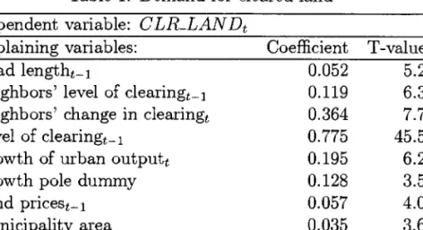
Table 1: Demand for cleared land

Dependent variable: CLR_LAND_t

Explaining variables: Coefficient T-value

Road lengtht_1 0.052 5.2

Neighbors' leveI of clearingt_l 0.119 6.3

Neighbors' change in clearingt 0.364 7.7

LeveI of clearingt_l 0.775 45.5

Growth of urban outputt 0.195 6.2

Growth pole dummy 0.128 3.5

Land priCeSt-l 0.057 4.0

Municipality area 0.035 3.6

Adjusted R2 0.876

The amount of cleared land is mainly determined by the demand for agricul-tural land, which in turn depend on the expected profitability of that land. The profitability depends on factors such as accessibility, availability, market condi-tions, and fiscal incentives.

Accessibility of land in a particular municipality was captured by road length in that municipality and by the clearing situation in neighboring municipalities. Access is being rapidly improved when the leveI and the speed of clearing is high in neighboring municipalities. All three variables have the expected sign and are highly significant.

The coefficient of the lagged leveI of clearing is positive but significant1y lower than unity. This is evidence of the saturation effect. As the leveI of clearing gets high, less forest is available for new clearing.

Economic prospects in a region are captured by urban output growth which indicates favorable local market conditions. The fiscal incentives in growth poles also has a significant1y positive effect on demand for agricultural land.

High land prices were expected to dampen the demand for cleared land, but the land price variable gets a significant1y positive coefficient. This may be be-cause high land prices is associated with good economic prospects which would add to the demand for cleared land.

The size of the rural population is mainly determined by the size of the rural population in the previous period. Population pressure from neighboring munic-ipalities is ais o very important, as shown by the highly significant coefficient to neighbors' change in rural population. Market conditions in the municipality are captured by urban income per urban capita and the growth rate of urban output. Finally, accessibility is captured by neighbors' change in road length.

t

Table 2: Rural population equation

Dependent variable: PO P -RU RALt

Explaining variables: Coefficient T-value

Constant -0.513 -7.2

Rural populationt_l 1.009 134.4

Urban income per urban capitat-l 0.041 5.1

Growth of urban outputt 0.103 9.5

Municipalityarea 0.016 4.1

Neighbors' change in rural populationt 0.691 15.0

Neighbors' change in road lengtht 0.027 3.0

Adjusted R2 0.965

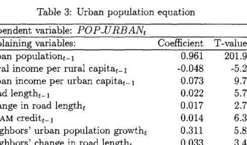
Table 3: Urban population equation

Dependent variable: _POP-URBANt

Explaining variables: Coefficient T-value

Urban populationt_l 0.961 201.9

Rural income per rural capitat_l -0.048 -5.2

Urban income per urban capitat-l 0.073 9.7

Road lengtht_1 0.022 5.7

Change in road lengtht 0.017 2.7

FIN AM credi tt-l 0.014 6.3

Neighbors' urban population growtht 0.311 5.8

Neighbors' change in road lengtht 0.033 3.4

Municipalityarea 0.025 5.5

Adjusted R2 _0.978

The size of the urban population depends mainly on last periods urban pop-ulation and on urban poppop-ulation growth in neighboring municipalities. Accessi-bility is captured by road length, new road building, and new road building in neighboring municipalities, which all have significantly positive coefficients.

The economic attractiveness of urban life in a municipality is captured by

urban income per urban capita and by the leveI of FINAM credito If rural income

per rural capita is high it becomes relatively less attractive to move to the city, as indicated by the negative coefficient on rural income per rural capita.

Rural output is mainly explained by the rural population and the average productivity of rural persons in the previous period.

The extension of the road network and the length of main rivers do not have significant effects on rural output. New road building, however, adds to rural output because it gives access to new forest which can be cleared and mined for nutrients. Yields are in general high the first few years after forest-burning, but

..

,

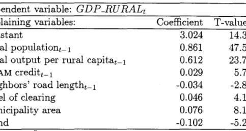
Table 4: Rural output equation

Dependent variable: G D P -RU RALt

Explaining variables: Coefficient T-value

Constant 3.024 14.3

Rural populationt_l 0.861 47.5

Rural output per rural capitat-l 0.612 23.7

FINAM creditt_l 0.029 5.7

N eighbors' road lengtht_1 -0.034 -2.8

LeveI of clearing 0.046 4.1

Muni ci pali ty area 0.076 8.1

Trend -0.102 -5.2

Adjusted R2 0.814

drops sharply thereafter unless artificial fertilizers are supplied.

Subsidized credit has a significantly positive effect on rural output, as ex-pected. The negative coefficient on neighbors' road length is unexex-pected.

The trend term gets a significantly negative coefficient, indicating either that the rural sector has experienced a general fall in productivity over the 1970-1985 period or that it has experienced a general deterioration in the terms of trade. Studies of the productivity of different kinds of land uses in the Amazon show that the productivity of both pasture land and crop land has increased steadily during that period. However, there has been a change in the composition of land uses in favor of cattle ranching which is, by far, the least productive land use in Amazonia. This change in composition can explain the overall fall in productivity

(Andersen et al (1996)).

Table 5: Urban output equation

Dependent variable: _GDP-URBANt

Explaining variables: Constant

Urban populationt_l

Urban output per urban capitat_l

FINAM creditt_l

Rural in come per rural capitat_l Urban environment Adjusted R2 Coefficient 2.495 0.905 0.796 0.052 -0.159 0.417 0.890 T-value 10.5 48.8 34.0 8.3 -6.0 4.7

Urban output is mainly explained by urban population and their productivity in the previous period. A good infrastructure adds to the leveI of urban output as does government incentives in the form of subsidized credito The negative

coefficient on rural income per rural capita shows that a relatively rich rural population is bad for urban output.

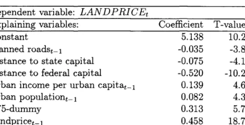
Table 6: Land price equation

Dependent variable: LAN D P RI C Et

Explaining variables: Constant

Planned roadst-1

Distance to state capital Distance to federal capital

Urban income per urban capitat_l Urban populationt_l T75-dummy Landpricet_l Adjusted R2 Coefficient 5.138 -0.035 -0.075 -0.520 0.139 0.082 0.313 0.458 0.466 T-value 10.2 -3.8 -4.1 -10.2 4.6 4.3 5.7 18.7

Land prices are mainly predicted from last periods land price, but location is also important. The farther away from Brasília, the lower the land prices, and the farther away from each state capital the lower the land prices. A relatively big urban population pushes up the land prices, especially if they are also relatively wealthy.

The negative coefficient on planned roads supports the argument made in

Section 2.4 on scarcity value. If people expect new land to be opened up by

new road building, then the already cleared land does not generate much scarcity value and, consequently, the pressure on land prices is lower.

Finally we get a significantly positive coefficient on the dummy for the 1975 period. This could be explained by a host of factors, but the most obvious is a relative change in the land prices in the rest of Brazil compared to the land

prices in the Amazon. If land prices in the rest of Brazil increased relatively fast

in the 1970-1975 period, this would but upward pressure on the land prices in the Amazon also. This was indeed the case. Land prices in the south increased so rapidly during the 1970-1975 period, that the gap between the South and the North increased from 1.7 in 1970 to 8.7 in 1975. In the following two five year periods, the gap remained around that leveI, and in 1985 the gap South-North

land price gap was about 8.110.

5. Predictions for 1985 - 2010

The model estimated in the previous section can be used to make rough predic-tions on the leveI and location of future land clearing in the Amazon.

•

Because of the linearity assumption, there is no built-in limit to the leveI of clearing that the model predicts. When predicted cleared are a exceeds 100% of municipality area, the predicted are a is therefore set equal to municipality area.

Predictions are made for two basic scenarios. One in which the aggressive development policies of the 1970-1985 period is continued in the following 25 years, and one in which they are seriously reduced or abandoned .

Scenario 1: Active development policies in the Amazon maintained. The assumptions made for scenario 1 are the following:

• Planned roads in 1985 are built evenly over the following 25 years.

• New roads continue to be planned, so that the amount of planned roads stay constant at the 1985 leveI.

• FINAM credit continues at the 1985 leveI. • Growth pole incentives are maintained.

• The urban infrastructure index is assumed to remain at the 1980 leveI, because a rapid urban population growth makes it impossible to improve housing conditions above that leveI.

• The land price gradient compared to the rest of Brazil is kept at the same leveI as in 1980 and 1985.

• The negative trend in agricultural output is assumed to stagnate, since a further deterioration in rural productivity and rural-urban terms of trade seem unrealistic in the view of technical progress and rapidly growing urban populations.

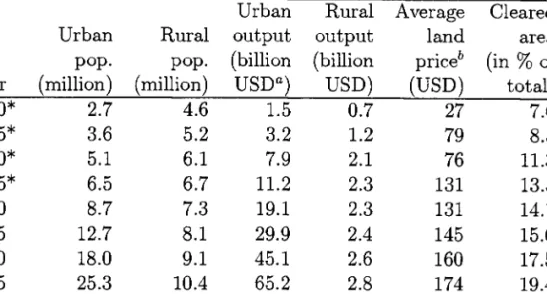
Using the estimated coefficients from the previous section together with the above assumptions about the exogenous variables, we get a cleared are a in year 2010 of 1.09 million square kilometers, or approximately 22 % of Legal Amazonia. The predicted behavior of the key variables is shown in Table 7.

The figures indicate a virtual explosion of the urban population. During the estimation period 1970-1985 the urban population already grew at an average annual rate of 6.1 %. In the forecasting period 1985-2010 this rate increased to 7.0% per year implying an urban population in the Amazon of about 35 million in the year 2010.

The rural population is predicted to grow at more modest rates. The average annual growth rate of 2.5% during the estimation period will more or less continue the following 25 years.

Real urban output is predicted to grow even faster than urban population. During the estimation period, urban output grew at an astonishing rate of 14.2%

1#

..

Table 7: Predictions under scenario 1

Urban Rural Average Cleared

Urban Rural output output land area

pop. pop. (billion (billion priceb (in % of

Year (million) (million) USDa) USD) (USD) total)

1970* 2.7 4.6 1.5 0.7 27 7.6 1975* 3.6 5.2 3.2 1.2 79 8.5 1980* 5.1 6.1 7.9 2.1 76 11.3 1985* 6.5 6.7 11.2 2.3 131 13.5 1990 8.7 7.3 19.1 2.3 131 14.1 1995 12.7 8.1 29.9 2.4 145 15.6 2000 18.0 9.1 45.1 2.6 160 17.5 2005 25.3 10.4 65.2 2.8 174 19.4 2010 35.4 11.9 91.4 3.1 186 21.5

a All values are in fixed 1985-USD. bWeighted by municipality size.

*

per year. The predicted annual growth rate of urban output during the following 25 years is 8.8%.

The growth rate of rural output was drastically reduced in the eighties com-pared to the seventies, and this lower growth rate is predicted to continue during the prediction period with average annual growth rates of only 1.2%. This is clearly not enough to feed the rapidly expanding urban population, so food im-ports will be necessary under this scenario.

Scenario 2: Active developrnent policies in the Arnazon abandoned. The assumptions made for scenario 2 are the following:

• The roads planned in 1985 are never built. The total amount of federal and state roads remain constant at the 1985 leveI.

• No new roads are being planned.

• FINAM credit drops to zero .

• Growth pole incentives are abandoned.

• The urban infrastructure index is assumed to remain at the 1980 leveI. • The land price gradient compared to the rest of Brazil is kept at the same

leveI as in 1980 and 1985.

11

•

..

•

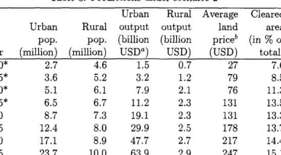
U sing the estimated coefficients from the previous section together with the above assumptions about the exogenous variables, we get a cleared area in 2010

of 0.80 million square kilometers, or approximately 16

%

predicted behavior of the key variables is shown in Table 8. Table 8: Predictions under scenario 2

Urban Rural Average Cleared

Urban Rural output output land area

pop. pop. (billion (billion priceb (in

%

Year (million) (million) USDa) USD) (USD) total)

1970* 2.7 4.6 1.5 0.7 27 7.6 1975* 3.6 5.2 3.2 1.2 79 8.5 1980* 5.1 6.1 7.9 2.1 76 11.3 1985* 6.5 6.7 11.2 2.3 131 13.5 1990 8.7 7.3 19.1 2.3 131 13.3 1995 12.4 8.0 29.9 2.5 178 13.7 2000 17.1 8.9 47.7 2.7 217 14.4 2005 23.7 10.0 63.9 2.9 247 15.1 2010 32.4 11.4 88.2 3.1 271 15.8

aAll values are in fuced 1985-USD. bWeighted by municipality size.

*

The dramatic change in assumptions on federal development policy had very

little effect on population growth and output growth. It did nevertheless reduce

the amount of cleared land considerably. Clearing in the year 2010 is reduced by 27% compared to scenario 1, while total output and total population are only reduced by 3% and 7%, respectively.

Even though the negative trend for rural productivity was assumed to leveI off under both scenarios, agricultural production per capita is predicted to fall dra-matically. In view of the recent productivity improvements experienced in older

settlements in the Amazon regionl l _{and the dramatic urbanization predicted, it}

may be reasonable to assume that the negative trend in rural productivity not only stagnates after 1985 but is actually reversed. Such a reversal would lead to a bigger and more realistic increase in rural output and a corresponding drop in

urban output12.

llSee, for example, Almeida and Uhl (1995) .

12It is not possible, with the current model, to give accurate quantitative information on the effects of changes in productivity and terms of trade, since these effects are only captured in a general trend termo

)I

•

•

6. Discussion

Several interesting points are highlighted by the predictions from the estimated model. Most important is probably the assertion that economic activity in the Amazon is not just policy-driven but based fundamentally on underlying market forces. The predictions show that a total abandonment of the aggressive develop-ment policies pursued in the 1960-1985 period, will imply only a small reduction in regional output compared to a situation of continued federal road building and continued subsidization of the region. The deforestation effect of government policy is not negligible however. Cleared area by the year 2010 is predicted to be 36% larger if the aggressive development policies are continued. This should be compared to a gain in regional output of less than 4%. This difference arises because the government policies tend to promote wasteful use of the land, while the private motivations driving urban and rural growth promote more effective use of the land. The difference between the two scenarios is almost 300,000 square kilometers of cleared land by the year 2010 - an area the size of Italy.

Another very interesting point is the impact of government policy on land prices. A sudden reduction in new road building implies that land along existing roads will develop scarcity value and land prices be pushed up. This is nicely captured by our model which predicts that average land prices in the year 2010 will be 46% higher if new federal road building is halted, compared to the situation where road building and the planning of new roads is continued at the 1985 level. It is also clear from the predictions that spatial correlation is very important. Clearing visibly takes place at a moving agricultural frontier, which moves from the highly cleared are as in the southern and eastern part of Legal Amazonia towards the still forested areas in the north-western parto Smaller frontiers can be seen to extend outwards from the major cities in the regions, most notably Manaus, Santarém, and Rio Branco.

The rapid population growth predicted under both scenarios require a con-tinued massive migration to the Amazon region. Assuming that the resident population in Legal Amazonia in 1985 grow at an average annual rate of 2.5% we need about 20 million migrants during the 1985-2010 period to fiU the gap. Schneider (1992, p. 9) argues that the pool of potential migrants will fall during that period because he assumes that migrants will continue to come mainly from rural areas. But that is not necessarily a good assumption, since 85% of the pop-ulation growth is predicted to take place in urban areas. Assuming a historically moderate average population growth rate of 2.0% for the whole of Brazil, there will be a total population increase of 85 million people during the 1985-2010 pe-riod. Considering the congestion of people in the megalopolises in the South and the concentration of land ownership, it is quite possible that a good fraction of these will move to the Amazon where real urban income per capita is predicted to grow at more than 1.8% per year.

•

•

..

•

•

References

Almeida, O. T. d. & Uhl, C. (1995), 'Developing a quantitative framework for

sustainable resource-use planning in the Brazilian Amazon', World

Devel-opment 23, 1745-1764.

Andersen, L. E. & Weinhold, D. (1996), Modelling the frontier-effect in

Ama-zon deforestation using spatial variables, Mimeo, Department of Economics, University of Aarhus, Denmark.

Andersen, L. E., Granger, C. W. J., Reis, E. J., Huang, L.-L. & Weinhold, D.

(1996), Report on Amazon deforestation, Discussion paper, Department of Economics, University of California - San Diego.

Binswanger, H. P. (1989), Brazilian policies that encourage deforestation in the

Amazon, Environment Department Working Paper 16, The World Bank.

Brown, K. & Pearce, D. W., eds (1994), The Causes of Tropical Deforestation,

London: UCL Press Limited.

Deacon, R. T. (1995), 'Assessing the relationship between government policy

and deforestation', Journal of Environmental Economics and Management

28, 1-18.

Fearnside, P. M. (1996), Deforestation in Brazilian Amazonia: Comparison of

recent landsat estimates, Draft, National Institute for Research in the Ama-zon, Manaus, Brazil.

Reis, E. J. & Guzman, R. M. (1994), An econometric model of Amazon

de-forestation, in K. Brown & D. W. Pearce, eds, 'The Causes of Tropical

Deforestation', London: UCL Press Limited.

Schneider, R. R. (1992), An economic analysis of environmental problems in the

I ~ I ,

•

,

•

N.Cham. P/EPGE SPE A544p

Autor: Andersen, Lykke E.

Título: Predicting Amazon deforestation through the

1111111111111111111111111111111111111111

~:!:

FGV _ BMHS N" Pat.:F2~/98