Is in ﬂation targeting a good remedy to control inﬂation? ☆

(1)

Is in

ﬂ

ation targeting a good remedy to control in

ﬂ

ation?

☆

Helder Ferreira de Mendonça

a,

_⁎

_{, Gustavo José de Guimarães e Souza}

b,c,1 a_{Fluminense Federal University, Department of Economics, National Council for Scienti}_ﬁ_{c and Technological Development (CNPq), Brazil} b_{University of Brasilia, Department of Economics, Brazil}

c_{Banco do Brasil, Brazil}

a b s t r a c t

a r t i c l e

i n f o

Article history:

Received 8 February 2009

Received in revised form 5 June 2011 Accepted 29 June 2011

JEL classiﬁcation: E42

E52

Keywords: Inﬂation targeting Credibility

Propensity score matching

Since the 1990s inflation targeting (IT) has been adopted by several central banks as a strategy for monetary policy. It is expected that the adoption of this monetary regime can reduce inflation and inflation volatility. This article is concerned with these issues and makes use of the Propensity Score Matching methodology on a sample of 180 countries for the period from 1990 to 2007. For analysis, the sample is split into two sets of countries (advanced and developing). Thefindings suggest that the adoption of IT is an ideal monetary regime for developing economies and, in addition to reducing inflation volatility, can drive inflation down to internationally acceptable levels. Regarding advanced economies, the adoption of IT does not appear to represent an advantageous strategy. In brief, the empirical results indicate that the adoption of IT is useful for countries that must enhance their credibility for the management of monetary policy.

1. Introduction

Since the early 1990s, inflation targeting framework (IT) has been adopted by several central banks as a strategy for the implementation of monetary policy. IT has as its main feature the official announce-ment of ranges for inflationfluctuations and the explicit recognition that the main objective of monetary policy is to assure a low and stable inflation rate. This monetary regime works as a guide for inflation expectations and it is associated with an increase in central bank transparency, which, in turn, increases accountability in the implementation of monetary policy and thus improves the central banks' credibility.2

An important step in controlling inflation is to guide inflationary expectations, thus one main task of a central bank is to build credibility through the commitment to price stability. Credibility is important because it influences public expectations affecting interest and exchange rates and thereby improves the implementation of monetary policy and a lower and stable inflation rate.

Nowadays, there is a growing literature (both theoretical and empirical) that seeks to demonstrate the advantages and weaknesses of the IT regime. Nonetheless, the effectiveness of this framework for inflation control fuels a controversial debate between policymakers and academics. Two key questions remain unanswered in a conclusive way: (i) How successful is IT in reducing and stabilizing the inflation rate? (ii) Are effects caused by IT sufficiently homogeneous when both developing and industrialized countries are taken into consid-eration? The answer to these questions depends on the observation of the countries that have adopted IT; as such, the analysis is fundamentally empirical.

Although the empirical results are not always convergent, it is possible to identify a common element in the studies– the self-selection problem–which in turn may create a bias in the outcomes (Lin and Ye, 2007).3_{To mitigate the bias problem, this article adopts a} method used by the medical literature and that is typically used to solve microeconomic problems: Propensity Score Matching, or PSM (Rosenbaum and Rubin, 1983). PSM emerged from the theory of counterfactuals, which calculates possible outcomes for patients who do receive or do not receive a given medical treatment. Due to the logical impossibility of observing this situation, the solution is to estimate the event. Hence, the matching framework is adequate for

Journal of Development Economics 98 (2012) 178–191

☆ We thank Érica Amorim, two anonymous referees and the editor, William Easterly, for helpful comments on an earlier version of this article. Any remaining errors are the sole responsibility of the authors.

⁎ Corresponding author at: Rua Dr. Sodré, 59, Vila Suíça, Miguel Pereira, Rio de Janeiro, CEP: 26900-000, Brazil.

E-mail addresses:[email protected](H.F. de Mendonça),

[email protected](G.J. de Guimarães e Souza).

1_{SQS 408, Bloco G, Apto 203, Asa Sul, Brasília/DF, CEP: 71939-360, Brazil.} 2_See,_{Svensson (1997), Mishkin (1999), Bernanke et al. (1999), Landarretche et al.}

(2001), de Mendonça and Simão Filho (2007), and Blinder et al. (2008).

3_{This problem is due to the fact that the adoption of IT is voluntary. For a wide}

discussion about the problem and its origins, seeWooldridge (2002).

Contents lists available atScienceDirect

Journal of Development Economics

(2)

these cases. Moreover, the propensity score also serves as a strategy for overcoming selection bias problems in the estimations.

In comparing inflation to medicine, inflation can be seen as an analogy for a typical illness in capitalist economies. In a general way, inflation is an illness without a cure; that said, the illness can still be treated in order to control the symptoms. Under this view, IT can be understood as a remedy for stabilizing and controlling inflation. Hence, just as in medicine, this study involves a quasi-natural experiment in which it is analyzed whether the remedy (IT) leads to the desired effects, or whether observed outcomes derive from other factors. To shed light on this question, this article looks at countries that adopted inflation targeting (inflation targeters—ITers) to see whether the changes with respect to inflation/inflation volatility observed over time are really due to the adoption of IT.

With the above-mentioned objective in mind and with recourse to panel data methodology, a set of 180 countries is considered in the analysis of the period 1990 to 2007. Note that among these countries, 29 adopted IT during the period under consideration. Due to the difficulty in determining the date when each country adopted IT, this analysis conducts extensive research of the literature as well as consultation with all the respective central banks. As a consequence, two sets of data are used: one with the start date of partial adoption of inflation targeting (soft inflation targeting); another with the date of full adoption of inflation targeting (full-fledged inflation targeting).

The analysis in this paper employs the best-fitted methodology available in the literature, i.e., PSM. The sample is split into two sets of countries (advanced and developing countries), which provides, using the same database, distinct and comparable results.4_{Based on} the same methodology, it is therefore possible to evaluate whether the outcomes for countries under IT still remain when advanced and developing countries are analyzed separately. Additionally, cases of high inflation in the study are controlled with the objective of rendering a more robust analysis. In brief, it is expected that with the assessment of the conditions described above, this study can improve the analysis of effects on inflation and volatility exclusively caused by implementation of IT. The article is organized as follows:Section 3 summarizes the research in literature regarding (a) IT, and (b) central banks vis-à-vis the inflation targeting adoption date according to conceptual criteria.Section 3describes the matching method known as propensity score and the database. Section 4 presents the estimation of PSM models and reports the results regarding the evaluation of IT worldwide.Section 5concludes the article.

2. IT adoption date

Despite the extensive literature on IT, there is no consensus as to the exact date that IT was implemented for thefirst time. Indeed, varying criteria are used by academics and policymakers. Because the main contribution of this study is empirical, the correct identification of the period under treatment (period under IT) is crucial; thus this study considers the information available in the inflation targeting literature and information from central banks regarding adoption date.

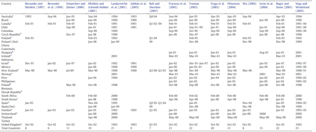
With the intention of avoiding the date-of-adoption problem and of strengthening this analysis, this study adopts two possible start dates for each country, as proposed byVega and Winkelried (2005). Thefirst set of dates refers to the period when the country announces a numerical target for inflation and the transition to IT is confirmed (soft IT). In this case, the monetary authority releases an inflation target to the public, although a set of policies that characterize a complete IT is not assumed (initial classification). The second set of

dates refers to complete adoption of IT (full-fledged IT). Full-fledged IT assumes explicit adoption of IT and the absence of other nominal anchors (conservative classification).

Table A.1(seeAppendix A) consolidates the data regarding the different dates of IT adoption for the countries considered in this study. The dates in the table were obtained through several studies concerning IT in the period 1997 to 2008. In cases where the literature and consultation with central banks present two distinct dates as to the date of adoption for a given country, the earlier date is considered as“initial”and the later is classiﬁed as“conservative.”5

As can be seen in Table A.1, the date of IT adoption is not homogenous among the sources. Even when the presence of one or two authors is observed in different articles, there are different dates for several countries.6_{The reason for this concerns the option} of some countries using a transition period leading up to full-ﬂedged IT. In a general way, the dates in advanced countries are less controversial because a transition period is not adopted. This behavior is evidenced by the difference in years between the two classiﬁcations used. For the set of countries that adopted IT, the average difference is 1.7 years; for the 17 developing countries, the difference is 2 years; and for the 12 advanced countries, the difference is 1.3 years.

3. Methodology

Over time, the experience of countries that have adopted IT, as well as the number of ITers, increases. This burgeoning database is a fertile ground for new possibilities for measuring the IT effects on inflation; consequently, the empirical literature includes myriad ways to exhibit results. For example,Landarretche et al. (2001)conduct an empirical study through the use of Vector Autoregression Analysis (VAR) regarding the advantages of IT adoption for the period 1980 to 1999 for three sets of countries (ITers, potential ITers, and non-ITers) in a total sample of 25 countries. They found that ITers have been successful in meeting targets and have consistently reduced inflation-forecast errors. Johnson (2002)comparesfive ITers with six non-ITers from 1984 to 2000, based on dummy coefficients; it was found that inflation targets correlated with disinflation and smaller forecast errors. In the same way, Neumann and von Hagen (2002)take into consideration six industrial ITers and three non-ITers, quantifying the response of inflation on supply shocks; they found evidence that ITers reduced inflation to low levels and curbed inflation and interest rate volatility.

Taking into account a sample of 21 ITers,Pétursson (2004)uses a dummy variable for the period after the adoption of IT with the objective of evaluating the performance of macroeconomic indicators. Under this view, IT is successful and increases the probability that monetary policy can engender good decision-making, thereby improving the credibility of monetary policy. Levin et al. (2004) considered 11 industrialized countries (including five ITers) in analyzing the effect caused by IT on the persistence of inflation through a univariate autoregressive process. They found that IT has played a role in anchoring inflation expectations and in reducing inflation persistence. Based on a sample of 14 full-fledged ITers,de Mendonça (2007a)analyzed macroeconomic performance before and after adoption of IT and concluded that IT is a good framework for disinflation, and contributes to reducing interest rates without curtailing economic growth.

4_{The division is made taking into consideration the classi}_ﬁ_{cation made by the} International Monetary Fund (IMF).

5_{Due to their entrances into the European Union, the abandon date of IT by Finland}

and Spain is also shown.

6_{For example, South Africa, Australia, Spain, Israel, and Sweden (see}_{Bernanke et al.,}

1999; Bernanke and Mishkin, 1997; Landarretche et al., 2001; Mishkin and Schmidt-Hebbel, 2001, 2007).

(3)

The main problem with the abovementioned studies is due to the arbitrary selection of countries that have not adopted IT for purposes of comparison with countries that have adopted IT, or because the study analyzes a country before and after IT adoption.7_{Moreover, the} studies mentioned do not address the problem of self-selection and, thus, suffer from potential bias in the results.

Few studies take into consideration the choice of counterfactuals. Ball and Sheridan (2003)use the difference-in-differences method for 20 OCDE countries (where 7 are ITers).Gonçalves and Salles (2008) extend the same analysis to 36 developing countries (where 13 are ITers).Vega and Winkelried (2005)use the PSM method for a sample of 109 countries (23 ITers) for the period 1990 to 2004. However, because the authors use an average ofﬁve years for model variables, the result is based on a mere 100 observations, which in turn, entails few counterfactuals (33 on average for each model). Lin and Ye (2007)employ PSM analysis for seven industrial countries that have adopted IT out of a total sample of 22 countries for the period 1985 to 1999 (total of 321 observations).

The above review of the literature reveals that the majority of studies concerning IT fails to consider problems caused by selection bias. The few studies that do take the problem into consideration are compromised by (a) too-short a window of analysis; (b) too-few countries implementing IT; (c) insufﬁcient quantity/quality of counterfactuals; and (d) outcomes that enable a comparison to be made between advanced and developing countries. In this study, the PSM framework (the most suitable for analyzing inﬂation and its volatility under IT),8 _{a greater number of treatment and control} countries, and a more extensive period of time including recent experiences with IT are considered. Moreover, temporal control variables, which constitute the context of IT implementation worldwide, are embedded in the model. The full panel data framework shows information of 180 countries for the period 1990 to 2007, i.e., 3240 observations. In relation to the 30 advanced countries in the sample, 12 have already adopted IT. Among the 150 developing countries in the analysis, 17 have adopted IT. Therefore, this study considers the experience of 29 countries under IT treatment (at the time of writing, the largest sample of ITers studied thus far– seeTable A.1–appendix).

The matching method consists of the selection of an ideal control group based on a treatment group. The idea is that for each country that has adopted IT, there is a counterfactual for comparison. However, the statistical literature recognizes that the estimation of a casual effect through the comparison of a treatment group with a control group (non-experimental) can be biased, either due to the selectivity problem or due to some systematic bias by researchers when selecting for matching.

The abovementioned bias can appear a consequence of the difference between ITers and non-ITers, which in turn, can affect the choice for adopting IT as well as its subsequent performance, and causing problems with sample selection. Therefore, the matching method considers distinct sets that are alike, based on their observable characteristics, and that allows ﬁnding non-biased estimation. In this sense, due to the high-dimensional covariate vectors needed for the objective of this study, the PSM method is the preferred option (Dehejia and Wahba, 2002).

It is important to note that the estimation of the propensity score does not attempt to ﬁnd the best model that can provide the probability of adopting IT. According toPersson (2001, p. 441)“the objective […] is not to build a statistical (let alone an economic or political) model explaining […] in the best possible way […] in fact, a

close to perfect fit […] would be destructive for the matching approach.”9_{Therefore, the variables that determine only the} proba-bility of IT being adopted by a central bank are not used. The set of characteristics may influence the probability of adopting IT and also the average and volatility of inflation. In addition, variables that characterize and summarize the state of the economy are also considered.

The key question when using this methodology is, had the country not adopted IT, would it have achieved the same results with respect to inﬂation and inﬂation volatility? Based on a methodology that simulates a pseudo-natural experiment, it should be possible to answer this question.

3.1. Data

The panel data present in this study includes information from 180 countries from 1990 to 2007 (see appendix—Table A.1to ITers and Table A.2to non-ITers). Due to the methodology adopted, it makes little sense to extend the sample to the years before the 1990s. This is because before the 1990s, the likelihood of adopting IT was low due to a lack of theoretical development and practical application. The data was gathered from the following sources: World Development Indicators (WDI); International Financial Statistics (IFS);Reinhart and Rogoff (2004); Ilzetzki et al. (2008); and Chinn and Ito (2008).10 Based on an analysis of the probability of adoption of IT and the effects of IT on inﬂation, the following variables were deﬁned for the PSM11_:

(i) GDPP — per capita GDP12 _{of the country; GDPP can be} understood as a universal measure of economic development. Leyva (2008) emphasizes that this variable can work as a general indicator of institutional development for substituting the indices of autonomy or central bank credibility13_; (ii) GFB — government ﬁscal balance (per cent of GDP); it is

assumed that GFB avoids the monetization process and thus is one precondition to the success of IT.14_{Under this view, the} control of money is not a sufficient condition to determine the path of inflation. According toWoodford (2001, p. 724),“a central bank charged with maintaining price stability cannot be indifferent as to howfiscal policy is determined;”

(iii) MONEY—ratio of M2/GDP; based on a monetarist view, it is expected that an increase in this ratio implies pressure on inﬂation;

(iv) KAOPEN —a measure of financial openness; the degree of integration of a country to international capital markets may affect the way countries react to international shocks, the effectiveness of its monetary (or exchange rate) policy and, ultimately, the rate of inflation. The argument holds that due to financial globalization, competition among currencies helps induce central banks to adopt best practices and keeps inflation low (Tytell and Wei, 2004);

(v) TRADE —a measure of commercial openness; TRADE corre-sponds to the exportation plus importation of goods and services (percent of GDP). As suggested, for example, byRomer

7_{It is important to note that when the in}_ﬂ_{ation of a country is compared before and} after IT adoption, the observed change can be a result of factors other than the adoption of the monetary regime.

8_{Appendix A.1 shows the explanation of the PSM methodology used in this study.}

9_{See also,}_{Vega and Winkelried (2005), and Lin and Ye (2007)}_.

10_{Other sources also considered in the analysis were Penn World Table (PWT 6.3),}

andGhosh et al. (2003); however, for reasons of parsimony, this information was not considered in theﬁnal speciﬁcations of the models.

11_{The studies considered are}_{Vega and Winkelried (2005), Hu (2006), Lin and Ye}

(2007), and Leyva (2008).

12_{Gross Domestic Product is the most commonly used single measure of a country's}

overall economic activity.

13_{For an analysis regarding these indices, see}_{Cukierman et al. (1992), Svensson and}

Faust (2001), Cecchetti and Krause (2002), de Mendonça (2007a), and de Mendonça and de Guimarães e Souza (2009).

(4)

(1993) and Rogoff (2003), more open economies reduces the inﬂation bias of central banks;

(vi) FER—fixed exchange rate; FER is a dummy variable equal to one when the country has some control over the exchange rate (e.g., currency board, crawling peg, de facto peg, etc.) and zero otherwise (e.g., managedfloating, freelyfloating, etc.); (vii) CPI−1—the previous inflation rate, as measured by Consumer

Price Index; lagged inﬂation is relevant in the model due to the fact that the magnitude of this variable has the power to inﬂuence the adoption of IT; used as a control for initial conditions.

In addition, with the intention of differentiating between the temporal characteristics and the international environment, which influence the decision to adopt IT and also affect the country's inflation and volatility, the following variables are also considered: TIME—a time dummy; WCPI—the world inflation rate; and WGDP— world GDP.

In brief, the covariates matrix chosen (a) characterizes the country's economy and maps the historical moment; (b) assures the random process concerning the choice of adopting IT; and (c) is systematically correlated with the outcomes of inﬂation and volatility. Given the foregoing, the conditions for estimation of PSM are assured.15

As a measure of inflation, the annual variation of Consumer Price Indexfigures released by the International Monetary Fund are used. Note that regarding inflation volatility, by reducing inflation, countries with a greater level of inflation can decrease the standard deviation, but not relative volatility (coefficient of variation); thus, the use of standard deviation is unsuitable in this case. Nonetheless, the coefficient of variation is not a perfect substitute, since it tends to balloon as inflation becomes very low. Hence, with the objective of mitigating an improper measurement and thus a false outcome in regard to inflation volatility, both standard deviation and coefficient of variation are employed in the estimations.16

4. Evaluation of IT in the world through a PSM model

Since the 1990s, a growing number of countries have adopted IT. The literature concerning IT suggests that the use of this strategy contributes to decreased inflation and inflation volatility. Table 1 shows the average inflation for the set of countries that adopted IT and for countries that adopted other strategies for the implementation of monetary policy in the period 1990 to 2007. The total sample concerns 180 countries, and the IT adoption date is based on initial classification. In addition,Table 1shows the same information for the case where the countries with high inflation are removed from the sample. The table takes into account two sets of countries: advanced and developing.

It is evident that average inﬂation, as well as average inﬂation volatility, is greater for the set of countries that did not adopt IT. The main reason for this outcome is due to the presence of developing countries in the sample.17_{Furthermore, it can be seen that although} the difference between ITers and non-ITers diminishes, it is not eliminated.

Taking into account the above considerations, a set of six models (compared one with the other, which allows an ample analysis from the results found) is estimated. The baseline model considers the dates of adoption of IT based on initial classiﬁcation (similar to dates

obtained from central banks) and original data (without any treatment). The second model uses dates of adoption of IT based on conservative classification. Hence, besides the comparison with the baseline model, the second model is also employed to make a specific analysis for the cases where there exists an explicit IT. The third model represents the baseline model without TRADE. The elimination of TRADE from the estimation is motivated by the fact that certain authors, e.g.,Wynne and Kersting (2007), argue that the discipline on central banks is a consequence offinancial globalization rather than real (goods and services) globalization. Therefore, the estimation without this variable provides assurance as to its relevance in the analysis. In an attempt to remove the presence of outliers from estimation, the fourth model eliminates the cases of high inflation (annual inflation rate greater than 40%).18Because the presence of outliers (very high inflation for a few countries) will be very influential in determining the results, and aiming to maintain the number of observations in the models, the fifth model takes into account the inflation“D”instead of percentage change in price level, as suggested byCukierman et al. (1992).19_{The sixth model, instead of} using time dummies (TIME) in order to control the Probit specifi ca-tion, includes worldwide variables (WCPI and WGDP).

Periods of high world inflation imply greater domestic inflation rates and thus the traditional mechanism for controlling the increase in domestic prices loses efficiency. Under such an environment, the monetary authority has a lower credibility and consequently demands a greater sacrifice rate for controlling the increase in prices. One possible outcome is that the adoption of a tight monetary policy, such as IT, may be inhibited, resulting in negative WCPI. On the other hand, it is expected that the sign of WGDP is positive, given that in global boom periods, better structural and institutional conditions for the adoption of IT prevail.

In relation to the other covariates that deﬁne the economy of the country, it is expected that GDPP, MONEY, KAOPEN, and TIME have positive signs in the estimations. As pointed out byTruman (2003), and Lin and Ye (2007), greater GDPP implies better conditions for the adoption of IT. The variable MONEY represents the degree to which the economy is monetized. Moreover, when this ratio is higher, greater competence by the government is implied in its programming of monetary policy in an effective way (Hu, 2006).20 _{In regard to} KAOPEN, an increase in a country's integration with international capital markets can work as an instrument in the control of inﬂation through an improvement in credibility (see Gruben and McLeod, 2002), thereby creating a favorable environment for the adoption of

15_{The variables chosen also take into account characteristics that the literature}

indicates as prerequisite conditions for the adoption of IT. See,Svensson (2002); Mishkin (2004); Truman (2003); and Lin and Ye (2007).

16_{Standard deviation and the coef}_ﬁ_{cient of variation for in}_ﬂ_{ation rate are calculated} for the period of one year.

17_{The number of developing countries represents 83.33% of the total countries.}

18_{The classical de}_fi_{nition of hyperin}_fl_{ation is due to}_{Cagan (1956)}_{. The modern} classification of hyperinflation and high inflation used in this article is based onBruno and Easterly (1998), Fischer et al. (2002), and Reinhart and Savastano (2003).

19_“_D_”_{is the transformed in}_ﬂ_{ation rate and it takes a value from}_“₀_”_to_“₁_”_(D=_π_/(1+_π_)), whereπis the in_ﬂation rate.

20_{This ratio is useful to determine the ef}_ﬁ_{ciency of the}_ﬁ_{nancial system to mobilize} funds for economic growth (Bruno and Easterly, 1998).

Table 1

Inﬂation and its volatility (1990–2007).

Average All countries Advanced countries Developing countries Non-ITers Iters Non-ITers Iters Non-ITers ITers

All sample

CPI 78.25 5.03 3.26 2.76 92.95 6.82 CPI S.E. 49.10 1.12 0.60 0.75 58.54 1.41

Without high inﬂation

CPI 7.26 4.83 3.26 2.76 8.13 6.48 CPI S.E. 3.04 1.06 0.60 0.75 3.57 1.31 Note: S.E. is the standard error.“Without High Inﬂation”corresponds to the case of countries with inﬂation lower than 40% pa.

(5)

IT. At a minimum, a positive relation for TIME is expected because it captures the increase in the probability of adopting IT over time.

Contrary to the variables listed above, it is expected that the signs for GFB, TRADE, FER, and CPI−1 are negative. Fiscal control is a

necessary condition for achieving price stability. Therefore, contrary to the monetarist view, the determination of price level is afiscal phenomenon. Underpinning this theory is the hypothesis that the growth rate of public bonds explains the price level. Therefore, afiscal imbalance suggests a lower chance for the adoption of IT. Based on Vega and Winkelried (2005), and Lin and Ye (2007), the use of exchange rate targeting is more attractive to countries that are more open to trade; thus a negative coefficient of the variable TRADE is expected. As the use of afixed exchange rate regime is incompatible with IT, a negative sign for FER is expected. In regard to earlier inflation levels, high current inflation inhibits the adoption of IT because the use of a disinflationary strategy can have a high social cost; therefore, a negative sign is expected.

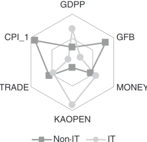
Fig. 1depicts the main characteristics of the variables present in the analysis, taking into account full data (developing and advanced countries). As indicated, GDPP and KAOPEN are greatest for the set of ITers. The opposite occurs when GFB and CPI−1are considered. No

reasonably clear interpretation of MONEY and TRADE is apparent. Nonetheless, in a general way, the variables used in the models behave differently when ITers and non-ITers are considered. There-fore, the distinction between the two sets regarding the effects of these variables in the estimation of the propensity score is confirmed. Table 2shows the estimations for the six models of propensity score. In a general way, independently of the specifications, the observed signs of the coefficients on the variables are in agreement with the theoretical view. The PSM models estimated using Probit present a good degree of fit and were approved in the diagnostic tests.21

It is observed that the tripod pertaining to the external side of the economy (KAOPEN-TRADE-FER) is relevant in the estimations. In particular, the worst speciﬁcation takes place when TRADE is taken out of the model (lowest pseudo R2_{, highest AIC and BIC).}

Furthermore, the following factors did not considerably change the outcomes achieved in the baseline model: (a) the use of models taking into account the conservative date in regard to the adoption of IT; (b) the elimination of countries with high inflation; and (c) the use of inflation“D”to mitigate the possible influence of outliers.

The results from the last model suggest that the use of time dummies as a control is preferable to the inclusion of variables such as WCPI and WGDP. Nonetheless, as expected, in the sixth specification, the coefficient on WCPI is negative, albeit with no statistical significance. In short, it is not safe to say that high WCPI is a disincentive to the adoption of IT. The coefficient on the other temporal control variable (WGDP) is positive, however, and does have statistical significance. Thus, moments of greater world economic activity correlate with a greater probability to adopt IT.

4.1. Average effect of treatment on the treated (ATT)

The ATT may be calculated after propensity score estimations. For each of the six PSM models, the average effects of adoption of IT for the ITers with respect to inflation and inflation volatility are reported. The ATT for each model is calculated based on by Stratification Matching, Nearest Neighbor-Matching, Radius Matching, and Kernel Matching estimators.22_{With the objective of increasing the sensitivity} in the analysis, an ample radius (r=0.10) and a lower radius (r=0.05) in Radius estimator are used, whereas in the Kernel estimator, the functions Gaussian and Epanechnikov are used.

Table 3summarizes the six models, taking into consideration the effects on inﬂation. Each model shows the outcomes of ATT for the average inﬂation with regard to the total sample, developing countries, and advanced countries. For a more detailed analysis of the effects of treatment (IT), the set of“matching”estimators was used. Despite the use of the common support condition (which improves the quality of matching, but reduces the number of observations), a great number of individuals for all models are available, which in turn improves the properties of PSM model.

Taking into account the total sample, the effect of the treatment on inflation is negative and has statistical significance independent of the estimator used for the six models. The most relevant reduction in the inflation average is observed by baseline model, which corresponds to 4 percentage points (hereinafter p.p.); the smallest reduction in the inflation average is presented by the model without the presence of high inflation (2.4 p.p.).23_{The same behavior is seen when the sample} of developing countries is considered in the analysis. In fact, the results are stronger than in the previous case: the highest fall in inflation is 6 p.p. (model“without trade”) and the lowest is 4.2 p.p. (model“high inflation”). It is important to stress that, when the outcomes found for advanced countries are analyzed separately, there is no empirical evidence that the presence of IT causes inflation to drop. This observation suggests that the result found in the total sample is influenced by developing countries.

In sum, the results considering “all sample” and “developing countries,”are strong and robust for the distinct PSM models and for different methods of matching. The evidence suggests that the adoption of full-ﬂedged IT, in opposition to soft IT, is advantageous for the case of developing countries. Furthermore, it is important to note that the use of controls for the cases of“conservative dates,” “without trade,” “high inﬂation,” “with D,” and “international controls” did not considerably change the results found by the baseline model.

It is expected that IT is capable not only of reducing inflation, but also of maintaining price stability. In this sense,Tables 3 and 4show the outcomes concerning inflation volatility (standard deviations and coefficient of variation, respectively). The stability contributes to improving the public's expectation of inflation and becomes an important mechanism for central banks to implement monetary

GDPP

GFB

MONEY

KAOPEN

TRADE

CPI_1

Non IT

IT

Fig. 1.Characteristics of the variables—full data.

21_{The value of 0.7 for an adjusted R}2_{of a model calculated through OLS can be}

compared to a value of 0.2 of a pseudo R2₍_{Louviere et al., 2000}_).

22_{The two manners for calculating the Nearest Neighbor estimator (equal weight}

and random draw) are identical, thus only one is reported.

23_{The analysis of comparison among the models excludes the model}_“_{with D}_” because its coefﬁcients do not allow a direct comparison with the others.

(6)

policy under IT.“As the most important step in controlling inflation is to control inflationary expectations, one main task of the [central bank] has been to build credibility as a monetary authority committed to price stability. Such credibility is important because it influences expectations affecting interest and exchange rates and thereby affects the cost of reducing inflation in terms of lost output and employment” (de Mendonça, 2007b, p. 2604).

The analysis regarding absolute volatility (standard deviations— Table 4) suggests that there is a significant decrease in volatility when the total sample and the case of developing countries are considered. Taking into account the total sample, the results indicate that the decrease in volatility is greater for the“baseline model,”while the decrease in volatility is lower for the“high inflation”model. In other words, when the countries with high inflation are removed from the sample (a typical case of developing economies) the consequence is a smaller impact on inflation volatility. Therefore, the results observed in the “all sample” model are explained in great measure by the performance of developing countries. In regard to developing economies, the model that captures the greater decrease in volatility is“international controls,”although the“without trade”model is very close. The smallest decrease in volatility is observed through the “baseline model.”

Contrary to the evidence above, the case of advanced countries suggests an increase in volatility due to the introduction of IT. Although the signiﬁcance is not as robust as in the previous cases, the use of counterfactuals indicates a very small increase in volatility in more than half of the models.24

With respect to relative volatility, measured by the coefficient of variation, the results are less conclusive than in the previous analysis. It can be seen that in the models “all sample” and “advanced countries,” the influence caused by adoption of IT on inflation volatility can be disregarded. Nonetheless, as in the analysis concerning absolute volatility, the models for developing economies

reveal significant influence of IT on inflation volatility. Thus, this observation strengthens the relevance of the analysis for developing economies.

With the intention of analyzing the main results from the ATTs reported in Tables 3–5, Table 6 presents a summary of the aggregate results of all matching models.25 _{There is no doubt} that the effect of the treatment on inflation has statistical significance and causes a decrease in the inflation rate when the total sample (average of −3.3 p.p.) and developing countries (average of −5 p.p.) are considered. In contrast, there is no evidence that the adoption of IT implies any effect on inflation in the case of advanced countries.26

Similar to the analysis concerning the effect of the treatment on inflation, the results from standard deviations suggest there is a significant decrease in inflation volatility for cases where the total sample (average of−1.5 p.p.) and developing countries (average of −2 p.p.) are considered. The evidence from the coefficient of variations is not as strong as that shown by the standard deviations. However, where significant results were observed, the models also provided evidence of a decrease in inflation volatility (especially for developing countries). The results for the advanced economies indicate a different behavior. In the case of the outcomes from standard deviations, the increase in inflation volatility, although small, cannot be ignored (average of 0.3 p.p.). The models with statistical significance for coefficient variation also suggest an increase in inflation volatility. A possible reason for this result is that in the case of advanced economies, credibility is already high, thus the central bank has more flexibility in the management of monetary policy.

In short, as in medical cases, the effects are not homogenous when different types of individuals are considered (here developing and advanced countries). The results suggest that for developing

Table 2

Propensity score estimations—Probit model.

Variables Baseline Conservative dates Without trade High inﬂation With D International controls Coef Robust

std. err.

Coef Robust std. err.

Coef Robust std. err. GDPP 0.0358⁎⁎⁎ _0.0083 _0.0398⁎⁎⁎ _0.0093 _0.0299⁎⁎⁎ _0.0073 _0.0394⁎⁎⁎ _0.0088 _0.0354⁎⁎⁎ _0.0083 _0.0368⁎⁎⁎ _0.0083

GFB −0.0466⁎⁎⁎ _0.0171 ₋_0.0713⁎⁎ _0.0203 ₋_0.0524⁎⁎⁎ _0.0132 ₋_0.0477⁎⁎⁎ _0.0177 ₋_0.0467⁎⁎⁎ _0.0171 ₋_0.0498⁎⁎⁎ _0.0174

MONEY 0.0019⁎ _0.0011 _0.0029⁎ _0.0017 ₋_0.0019 _0.0015 _0.0014⁎⁎ _0.0008 _0.0017⁎ _0.0010 _0.0017 _0.0018

KAOPEN 0.0928⁎⁎ _0.0424 _0.0211 _0.0459 _0.0928⁎⁎ _0.0409 _0.0765⁎ _0.0425 _0.0930⁎⁎ _0.0424 _0.0929⁎⁎ _0.0429

TRADE 0.0049⁎⁎⁎ _0.0013 ₋_0.0038⁎⁎⁎ _0.0014 ₋_0.0048⁎⁎⁎ _0.0013 ₋_0.0049⁎⁎⁎ _0.0013 _0.0049⁎⁎⁎ _0.0013

FER −1.1434⁎⁎⁎ _0.1330 ₋_{1. 3686}⁎⁎⁎ _0.1500 ₋_1.1458⁎⁎⁎ _0.1265 ₋_1.1308⁎⁎⁎ _0.1329 ₋_1.1440 _0.1337 ₋_1.1574⁎⁎⁎ _0.1324

CPI_1 −0.0213⁎⁎ _0.0085 ₋_0.0718⁎⁎⁎ _0.0133 ₋_0.0218⁎⁎⁎ _0.0081 ₋_0.0180⁎⁎ _0.0093 ₋_3.0423 _1.0167 ₋_0.0222⁎⁎⁎ _0.0085

TIME 0.0707⁎⁎⁎ _0.0158 _0.1446⁎⁎⁎ _0.0246 _0.0591⁎⁎⁎ _0.0145 _0.0707⁎⁎⁎ _0.0159 _0.0712 _0.0159

WCPI −0.0027 0.0151

WGDP 0.0275⁎⁎⁎ _0.0080

Observations 828 828 863 779 828 828

Common support [0.0069, 0.9064] [0.0211, 0.9548] [0.0056, 0.8107] [0.0093, 0.9084] [0.0073, 0.9059] [0.0067, 0.9097] Log pseudo likelihood −264.02 −196.86 −285.36 −258.04 −264.21 −263.32 Wald chi2 _134.16⁎⁎⁎ _136.78⁎⁎⁎ _140.35⁎⁎⁎ _129.63⁎⁎⁎ _133.87⁎⁎⁎ _134.59⁎⁎⁎

Pseudo R2 _0.3042 _0.4194 _0.2667 _0.2967 _0.3037 _0.3060

AIC 546.05 411.71 586.73 534.07 546.41 546.63

BIC 588.52 454.18 624.81 576.00 588.88 593.82

Correctly classiﬁed 0.8816 0.9082 0.8691 0.8793 0.8804 0.8804

Note: Pseudo R2_{is the McFadden's R}2_{, AIC is the Akaike information Criterion and BIC is the Bayesian information Criterion. The constants terms are included but not reported. The} balancing property is satisﬁed for every models. D_1 was used instead of CPI_1 in the model With D.

⁎ Indicate the signiﬁcance level of 10%.

⁎⁎Indicate the signiﬁcance level of 5%.

⁎⁎⁎Indicate the signiﬁcance level of 1%.

24_{Note that the analysis on developed countries is based on a small sample size,}

which, in turn, implies that the results cannot be considered deﬁnitive.

25_{Differently from the previous analysis, the model}_“_with_D_”_{considers the in}_ﬂ_ation (π=D/(1−D)) to permit a direct comparison of the averages.

26_{The average of the models do not present large differences, which in turn,}

strengthens the idea that the PSM speciﬁcations are correct.

(7)

Table 3

Estimations of the treatment effect by IT on inﬂation for ITers.

Countries Matching

Stratiﬁcation Nearest neighbor

Radius Kernel Stratiﬁcations Nearest neighbor

Radius Kernel

0.1 0.05 Gausssian Epanechnikov 0.1 0.05 Gausssian Epanechnikov 0.1 0.05 Gausssian Epanechnikov

Model Baseline Conservatives dates Without TRADE

All sample −3.422 −3.181 −6.996 −3.436 −3.378 −3.529 −3.770 −4.230 −2.637 −2.983 −3.655 −3.976 −3.870 −1.948 −5.689 −3.918 −3.591 −3.543 (1.197)⁎⁎⁎ _(1.890)⁎ _(2.219) _(1.124) _– _– _(2.071)⁎ _(1.340)⁎⁎⁎ _(1.569)⁎ _(1.353)⁎⁎ _– _– _(1.168)⁎⁎⁎ _(1.107)⁎ _(2.751)⁎⁎ _(2.187)

⁎ – –

[1.245]⁎⁎⁎ _[1.679] _[1.118]⁎⁎⁎ _[1.211]⁎⁎⁎ _[1.465]⁎⁎ _[1.409]⁎⁎ _[2.450] _[2.435]⁎ _[1.627] _[1.451]⁎⁎ _[1.761]⁎⁎ _[1.814]⁎⁎ _11.468]⁎⁎⁎ _[1.433] _[3.418]⁎ _[3.221] _[1.078]⁎⁎⁎ _[1.282]⁎⁎⁎

IT 142 142 105 96 142 142 118 118 83 69 118 118 144 144 122 112 144 144

Non-IT 616 74 612 612 616 616 380 66 380 380 380 380 671 89 670 670 671 671

All 758 216 717 708 758 758 498 184 463 449 498 498 815 233 792 782 815 815

Developing countries

−5.017 −4.766 −6.718 −6.780 −4.964 −5.560 −6.366 −6.564 −4.292 −4.469 −6.324 −6.372 −6.554 −3.406 −6.099 −8.164 −5.656 −6.016 (1.440)⁎⁎⁎ _(2.565)⁎ _(3.611)⁎ _(4.067)⁎ _– _– _(2.263)⁎⁎⁎ _(1.445)⁎⁎⁎ _(1.863)⁎⁎ _(2.589)⁎ _– _– _(1.851)⁎⁎⁎ _(1.896)⁎ _(4.666)⁎ _(4.666)⁎ _– _–

[1.242]⁎⁎⁎ _[3.399] _[5.140] _[5.185] _[1.328]⁎⁎⁎ _[1.587]⁎⁎⁎ _[1.839]⁎⁎⁎ _[2.359]⁎⁎⁎ _[1.635]⁎⁎⁎ _[1.672]⁎⁎⁎ _[1.687]⁎⁎⁎ _[2.120]⁎⁎⁎ _[2.311]⁎⁎⁎ _[3.454] _[4.809] _[6.196] _[1.573]⁎⁎⁎ _[1.951]⁎⁎⁎

IT 90 90 84 72 90 90 70 72 56 46 72 72 90 90 79 69 90 90

Non-IT 565 60 565 565 565 565 336 48 334 334 334 334 600 68 539 539 600 600

All 655 150 649 637 655 655 406 120 390 380 406 406 690 158 618 608 690 690

Advanced countries

0.265 −0.058 0.142 −0.900 0.365 0.186 0.123 0.343 −1.355 −1.499 0.262 0.214 0.656 1.005 −0.682 −0.934 0.685 0.807 (0.403) (0.782) (0.394) (1.284) – – (0.487) (0.680) (0.826) (1.378) – – (0.549) (0.785) (0.574) (1.180) – –

[0.427] [0.408] [0.382] [1.280] [0.380] [0.433] [0.549] [0.411] [0.866] [1.132] [0.314] [0.438] [0.495] [0.633] [0.748] [1.034] [0.495] [0.583]

IT 52 52 52 13 52 52 46 46 18 13 46 46 53 54 25 17 54 54

Non-IT 35 14 35 35 35 35 42 12 42 42 42 42 57 21 56 56 56 56

All 87 66 87 48 87 87 88 58 60 55 88 88 110 75 81 73 110 110

Model High inﬂation With D International controls

All sample −2.439 −2.644 −2.362 −1.966 −2.532 −2.613 −0.022 −0.026 −0.029 −0.031 −0.022 −0.021 −3.697 −2.217 −7.142 −3.624 −3.378 −3.587 (0.876)⁎⁎⁎ _(2.661) _(0.638)⁎⁎⁎ _(0.894)⁎⁎ _– _– _(0.007)⁎⁎⁎ _(0.018) _(0.008)⁎⁎⁎ _(0.010)⁎⁎⁎ _– _– _(1.317)⁎⁎⁎ _(2.241) _(2.812)⁎⁎ _(2.078)⁎ _– _–

[1.138]⁎⁎ _[1.955] _[0.802]⁎⁎⁎ _[0.921]⁎⁎ _[0.865]⁎⁎⁎ _[1.373]⁎ _[0.010]⁎⁎ _[0.017] _[0.008]⁎⁎⁎ _[0.010]⁎⁎⁎ _[0.011]⁎⁎ _[0.008]⁎⁎⁎ _[1.500]⁎⁎ _[1.266]⁎ _[2.820]⁎⁎ _[3.270] _[1.507]⁎⁎ _[1.390]⁎⁎

IT 141 141 102 94 141 141 142 142 109 96 142 142 141 142 110 98 142 142

Non-IT 606 78 606 606 606 606 615 79 615 615 615 615 625 78 623 623 624 624

All 747 219 708 700 747 747 757 221 724 711 757 757 766 220 733 721 766 766

−4.726 −7.311 −1.941 −1.960 −4.123 −4.860 −0.032 −0.034 −0.024 −0.028 −0.033 −0.035 −5.528 −3.476 −7.743 −7.146 −4.967 −5.531 (1.151)⁎⁎⁎ _(2.896)⁎⁎ _(0.854)⁎⁎ _(1.025)⁎ _– _– _(0.010)⁎⁎⁎ _(0.017)⁎⁎ _(0.010)⁎⁎ _(0.011)⁎⁎ _– _– _(1.935)⁎⁎⁎ _(1.822)⁎ _(4.338)⁎ _(3.882)⁎ _– _–

[1.486]⁎⁎⁎ _[2.667]⁎⁎⁎ _[0.979]⁎⁎ _[0.967]⁎⁎ _[1.153]⁎⁎⁎ _[2.034]⁎⁎ _[0.009]v _[0.016]⁎⁎ _[0.010]⁎⁎ _[0.012]⁎⁎ _[0.010]⁎⁎⁎ _[0.012]⁎⁎⁎ _[1.769]⁎⁎⁎ _[1.952]⁎ _[4.540]⁎ _[4.767] _[1.580]⁎⁎⁎ _[1.678]⁎⁎

IT 90 90 79 74 90 90 90 90 78 76 90 90 88 90 81 69 90 90

Non-IT 555 59 555 555 555 555 564 65 564 564 564 564 575 63 573 573 573 573

All 645 149 634 629 645 645 654 155 642 540 554 654 663 153 654 642 663 663

Advanced countries

0.282 0.050 −0.689 −0.900 0.369 0.286 0.002 0.000 −0.010 −0.012 0.003 0.002 0.437 0.491 −0.709 −1.187 0.404 0.398 (0.357) (0.811) (0.961) (1.309) – – (0.004) (0.007) (0.009) (0.011) – – (0.380) (0.668) (1.006) (1.031) – –

[0.451] [0.380] [0.966] [1.352] [0.364] [0.415] [0.004] [0.003] [0.009] [0.014] [0.004] [0.004] [0.384] [0.365] [0.921] [1.349] [0.325] [0.343]

IT 51 51 23 13 51 51 52 52 23 12 52 52 49 52 19 14 52 52

Non-IT 35 15 35 35 35 35 35 14 35 35 35 35 34 16 31 31 31 31

All 86 66 58 48 86 86 87 66 58 47 87 87 83 68 50 45 83 83

Notes: 0.06ﬁxed bandwith is used for Epanechikov kernel. The analytical standard errors are reported in parenthesis and the bootstrapped standard errors are reported in brackets (they are based on 1000 replications of data).

⁎ _{Indicate the signi}_ﬁ_{cance level of 10%.} ⁎⁎ Indicate the signiﬁcance level of 5%.

⁎⁎⁎ Indicate the signiﬁcance level of 1%.

184

H.F.

de

Mendonça,

G.J.

de

Guim

arães

e

Souza

/

Journal

of

Development

Economics

98

(2012)

178

–

(8)

Table 4

Estimations of the treatment effect by IT on inﬂation volatility for ITers (standard deviations).

Countries Matching Stratiﬁcation Nearest

neighbor

Radius Kernel

Model Baseline Conservatives dates Without TRADE

All sample −1.183 −1.432 −4.980 −1.218 −1.113 −1.204 −1.439 −1.573 −1.059 −0.672 −1.406 −1.543 −1.182 −0.819 −5.522 −1.613 −1.160 −1.187 (0.460)⁎⁎ _(0.829)⁎ _(5.753) _(0.729)⁎ _– _– _(0.860)⁎ _(0.451)⁎⁎⁎ _(0.576)⁎ _(0.459) _– _– _(0.405)⁎⁎⁎ _(0.532)⁎ _(3.293)⁎ _(4.884) _– _–

[0.515]⁎⁎ _[0.7651⁎ _[2.865]⁎ _[0.877] _[0.536]⁎⁎ _[0.451]⁎⁎⁎ _[0.739]⁎ _[1.125] _[0.788] _[0.601] _[0.582]⁎⁎ _[0.816]⁎ _[0.402]⁎⁎⁎ _[0.515] _[4.104] _[4.672] _[0.329]⁎⁎⁎ _[0.334]⁎⁎⁎

IT 142 142 105 96 142 142 118 118 83 69 118 118 144 144 122 112 144 144

Non-IT 616 74 612 612 616 616 380 66 380 380 380 380 671 89 670 670 671 671

All 758 216 717 708 758 758 498 184 463 449 498 498 815 233 792 782 815 815

−1.799 −2.071 −5.073 −5.968 −1.725 −1.941 −2.607 −2.763 −0.878 −0.921 −2.552 −2.613 −2.077 −1.480) −5.582 −7.534 −1.911 −2.040 (0.490)⁎⁎⁎ _(0.769)⁎⁎⁎ _(5.586) _(4.811) _– _– _(0.727)⁎⁎⁎ _(0.493)⁎⁎⁎ _(0.459)⁎ _(0.927) _– _– _(0.689) _(0.591) _(3.070) _(11.697) _– _–

[0.445]⁎⁎⁎ _[0.966]⁎⁎ _[6.020] _[7.917] _[0.513]⁎⁎⁎ _[0.566]⁎⁎⁎ _[0.749]⁎⁎⁎ _[0.871]⁎⁎⁎ _[0.755] _[0.927] _[0.687]⁎⁎⁎ _[0.988]⁎⁎⁎ _[0.644]⁎⁎ _[0.310] _[0.175]⁎ _[0.263] _[0.115]⁎⁎⁎ _[0.151]⁎⁎

IT 90 90 84 72 90 90 70 72 56 46 72 72 90 90 79 69 90 90

Non-IT 565 60 565 565 565 565 336 48 334 334 334 334 600 68 539 539 600 600

All 655 150 649 637 655 655 406 120 390 380 406 406 690 158 618 608 690 590

Advanced countries

0.248 0.270 0.255 0.051 0.294 0.234 0.313 0.303 0.262 0.061 0.297 0.303 0.293 0.321 0.076 −0.024 0.290 0.288 (0.1.33)⁎ _(0.186) _(0.215) _(0.235) – – (0.157)⁎⁎ _(0.202) _(0.231) _(0.444) – – (0.102) (0.101) (0.171) (0.245) – –

[0.142]⁎ _[0.131]⁎⁎ _[0.294] _[0.338] _[0.101]⁎⁎⁎ _[0.147] _[0.139] _[0.126] _[0.327] _[0.291] _[0.107]⁎⁎⁎ _[0.130]⁎⁎ _[0.108]⁎⁎⁎ _[0.106]⁎⁎⁎ _[0.193] _[0.224] _[0.096]⁎⁎⁎ _[0.104]⁎⁎⁎

IT 52 52 52 13 52 52 46 46 18 13 46 46 53 54 25 17 54 54

Non-IT 35 14 35 35 35 35 42 12 42 42 42 42 57 21 56 56 56 56

All 87 66 87 48 87 87 88 58 60 55 88 88 110 75 81 73 110 110

All sample −0.884 −0.795 −0.951 −0.738 −0.887 −0.927 −0.008 −0.008 −0.007 −0.006 −0.007 −0.007 −1.175 −0.789 −5.173 −1.422 −1.067 −1.142 (0.377)⁎⁎ _(0.702) _(0.253)⁎⁎⁎ _(0.326)⁎⁎ _– _– _(0.003)⁎⁎⁎ _(0.004)⁎⁎ _(0.003)⁎⁎ _(0.003)⁎ _– _– _(0.443)⁎⁎⁎ _[0.464]⁎ _(3.140)⁎ _(3.240) _– _–

[0.450]⁎⁎ _[0.433]⁎ _[0.216]⁎⁎⁎ _[0.276]⁎⁎⁎ _[0.434]⁎ _[0.457]⁎⁎ _[0.003]⁎⁎⁎ _[0.005] _[0.003]⁎⁎ _[0.003]⁎ _[0.004]⁎ _[0.003]⁎⁎ _[0.545]⁎⁎ _[0.460]⁎ _[4.228] _[4.484] _[0.345]⁎⁎⁎ _[0.508]⁎⁎

IT 141 141 102 94 141 141 142 142 109 96 142 142 141 142 110 98 142 142

Non-IT 606 78 606 606 606 606 615 79 615 615 615 615 625 78 623 623 624 624

All 747 219 708 700 747 747 757 221 724 711 757 757 766 220 733 721 766 766

−1.781 −2.619 −1.002 −1.065 −1.574 −1.814 −0.012 −0.012 −0.010 −0.009 −0.012 −0.012 −1.844 −1.036 −5.210 −6.782 −1.682 −1.839 (0.438)⁎⁎⁎ _(0.834)⁎⁎⁎ _(0.334)⁎⁎⁎ _(0.323)⁎⁎⁎ – – (0.003)⁎⁎⁎ _(0.004)⁎⁎⁎ _(0.003)⁎⁎⁎ _(0.004)⁎⁎ – – (0.584)⁎⁎ _(0.462)⁎⁎ _(4.528) _(4.194) – –

[0.464]⁎⁎⁎ _[1.003]⁎⁎⁎ _[0.278]⁎⁎⁎ _[0.366]⁎⁎⁎ _[0.424]⁎⁎ _[0.648]⁎⁎⁎ _[0.003]⁎⁎⁎ _[0.004]⁎⁎⁎ _[0.004]⁎⁎ _[0.004]⁎⁎ _[0.003]⁎⁎⁎ _[0.004]⁎⁎⁎ _[0.608]⁎⁎⁎ _[0.585]⁎ _[6.414] _[4.020]⁎ _[0.430]⁎⁎⁎ _[0.618]⁎⁎⁎

IT 90 90 79 74 90 90 90 90 78 76 90 90 88 90 81 69 90 90

Non-IT 555 59 555 555 555 555 564 65 564 564 564 564 575 63 573 573 573 573

All 645 149 634 629 645 645 654 155 642 640 554 654 663 153 654 642 663 663

Advanced countries

0.253 0.050 0.137 0.045 0.292 0.291 0.002 0.003 0.002 0.001 0.003 0.002 0.301 0.305 0.378 0.365 0.298 0.291 (0.105)⁎⁎ _(0.811) _(0.254) _(0.309) _– _– _(0.001)⁎⁎ _(0.002) _(0.002) _(0.002) _– _– _(0.096) _(0.178) _(0.214)⁎ _(0.279) _– _–

[0.132]⁎ _[0.380] _[0.288] _[0.312] _[0.097]⁎⁎ _[0.171]⁎ _[0.001]⁎⁎ _[0.001]⁎⁎⁎ _[0.003] _[0.003] _[0.001]⁎⁎⁎ _[0.001]⁎⁎ _[0.117]⁎⁎ _[0.102]⁎⁎⁎ _[0.292] _[0.387] _[0.080]⁎⁎⁎ _[0.130]⁎⁎

IT 51 51 23 13 51 51 52 52 23 12 52 52 49 52 19 14 52 52

Non-IT 35 15 35 35 35 35 35 14 35 35 35 35 34 16 31 31 31 31

All 89 66 58 48 86 86 87 66 58 47 87 87 830 68 50 45 83 83

Notes: 0.06ﬁxed bandwith is used for Epanechnikov kernel. The analytical standard errors are reported in parentheses and the bootstrapped standard errors are reported in brackets (they are based on 1000 replications of the data).

⁎⁎ Indicate the signiﬁcance level of 5%.

⁎⁎⁎ _{Indicate the signi}_ﬁ_{cance level of 1%.}

185

H.F.

de

Mendonça,

G.J.

de

Guim

arães

e

Souza

/

Journal

of

Development

Economics

98

(2012)

178

–

(9)

Table 5

Estimations of the treatment effect by IT on inﬂation volatility for ITers (coefﬁcient of variation).

Countries Matching

Stratiﬁcation Nearest neighbor

Radius Kernel

Model Baseline Conservative dates Without TRADE

All sample −0.118 −0.176 −0.092 −0.121 −0.121 −0.121 −0.046 −0.091 −0.203 −0.259 −0.064 −0.059 −0.298 −0.363 −0.360 −0.378 −0.347 −0.337 (0.116) (0.242) (0.150) (0.158) – – (0.107) (0.363) (0.164) (0.207) – – (0.211) (0.241) (0.270) (0.288) – –

[0.099] [0.116] [0.141] [0.158] [0.093] [0.101] [0.116] [0.173] [0.164] [0.228] [0.087] [0.124] [0.341] [0.416] [0.339] [0.372] [0.214] [0.170⁎⁎_]

IT 142 142 105 96 142 142 118 118 83 69 118 118 144 144 122 112 144 144

Non-IT 616 74 612 612 616 616 380 66 380 380 380 380 671 89 670 670 671 671

All 158 216 717 708 758 758 498 184 463 449 498 498 815 233 792 782 815 815

−0.309 −0.265 −0.221 −0.207 −0.279 −0.267 −0.245 −0.317 −0.456 −0.399 −0.250 −0.249 −0.346 −0.463 −0.307 −0.214 −0.356 −0.364 (0.134)⁎⁎ _(0.123)⁎⁎ _(0.208) _(0.219) _– _– _(0.138)⁎ _(0.410) _(0.242)⁎ _(0.316) _– _– _(0.129)⁎⁎⁎ _(0.194)⁎⁎ _(0.180)⁎ _(0.213) _– _–

[0.150]⁎⁎ _[0.153]⁎ _[0.185] _[0.239] _[0.145] _[0.126]⁎⁎ _[0.145]⁎ _[0.250] _[0.253]⁎ _[0.295] _[0.125]⁎⁎ _[0.134]⁎ _[0.144]⁎⁎⁎ _[0.310] _[0.175]⁎ _[0.263] _[0.115]⁎⁎⁎ _[0.151]⁎⁎

IT 90 90 84 72 90 90 70 72 56 46 72 72 90 90 79 69 90 90

Non-IT 565 60 565 565 565 565 336 48 334 334 334 334 334 68 539 539 600 600

All 655 150 649 637 655 655 406 120 390 380 406 406 406 158 618 608 690 690

Advanced countries

0.233 0.222 0.128 0.118 0.165 0.145 0.270 0.246 0.315 0.195 0.230 0.249 −0.141 −1.142 0.008 0.099 −0.275 −0.518 (0.185) (0.131)⁎ _(0.245) _(0.270) _– _– _(0.172) _(0.177) _(0.493) _(0.725) _– _– _(0.210) _(1.675) _(0.784) _(1.257) _– _–

[0.189] [0.190] [0.289] [0.339] [0.136] [0.194] [0.159]⁎ _[0.161] _[0.305] _[0.348] _[0.185] _[0.174] _[0.299] _[1.846] _[1.121] _[1.286] _[0.374] _[0.517]

IT 52 52 52 13 52 52 46 46 18 13 46 46 53 54 25 17 54 54

Non-IT 35 14 35 35 35 35 42 12 42 42 42 42 57 21 56 56 56 56

All 87 66 87 48 87 87 88 58 60 55 88 88 110 75 81 73 110 110

All sample −0.108 −0.104 −0.160 −0.106 −0.122 −0.113 −0.180 −0.001 −0.239 −0.255 −0.214 −0.200 −0.108 −0.132 −0.208 −0.348 −0.110 −0.109 (0.113) (0.373) (0.155) (0.150) – – (0.130) (0.207) (0.231) (0.227) – – (0.107) (0.272) (0.157) (0.215) – –

[0.111] [0.166] [0.160] [0.183] [0.102] [0.115] [0.190] [0.148] [0.236] [0.280] [0.170] [0.188] [0.125] [0.134] [0.137] [0.211]⁎ _[0.100] _[0.103]

IT 141 141 102 94 141 141 142 142 109 96 142 142 141 142 110 98 142 142

Non-IT 606 78 606 606 606 606 615 79 615 615 615 615 625 78 623 623 624 624

All 747 219 708 700 747 747 757 221 724 711 757 757 766 220 733 721 766 766

Developing countries −0.320 −0.269 −0.260 −0.336 −0.287 −0.269 −0.418 −0.125 −0.271 −0.355 −0.427 −0.402 −0.275 −0.205 −0.308 −0.189 −0.273 −0.266 (0.142)⁎⁎ _(0.372) _(0.148)⁎ _(0.023)⁎ _– _– _(0.199)⁎⁎ _(0.147) _(0.297) _(0.364) _– _– _(0.150)⁎ _(0.233) _(0.227) _(0.229) _– _–

[0.166]⁎ _[0.188] _[0.196] _[0.213] _[0.123]⁎ _[0.111]⁎⁎ _0.287 _[0.189] _[0.275] _[0.444] _[0.290] _[0.239]⁎ _[0.139]⁎⁎ _[0.316] _[0.179]⁎ _[0.197] _[0.154]⁎ _[0.111]⁎⁎

IT 90 90 79 74 90 90 90 90 78 76 90 90 88 90 81 69 90 90

Non-IT 555 59 555 555 555 555 564 65 564 564 564 564 575 63 573 573 573 573

All 645 149 634 629 645 645 654 155 642 640 654 654 663 153 654 642 663 663

Advanced countries 0.254 0.203 0.121 0.121 0.169 0.138 0.240 0.217 0.219 0.323 0.174 0.160 0.196 0.002 0.436 0.448 0.173 0.170 (0.168) (0.157) (0.346) (0.498) – – (0.165) (0.226) (0.245) (0.269) – – (0.185) (0.428) (0.280) (0.536) – –

[0.147]⁎ _[0.121]⁎ _[0.299] _[0.349] _[0.155] _[0.156] _[0.128]⁎ _[0.184] _[0.260] _[0.438] _[0.164] _[0.203] _[0.102] _[0.232] _[0.418] _[0.307] _[0.160] _[0.168]

IT 51 51 23 13 51 51 52 52 23 12 52 52 49 52 19 14 52 52

Non-IT 35 15 35 35 35 35 35 14 35 35 35 35 34 16 31 31 31 31

All 86 66 58 48 86 86 87 66 58 47 87 87 88 68 50 45 83

Notes: 0.06ﬁxed bandwith is used for Epanechnikov kernel. The analytical standard errors are reported in parentheses and the bootstrapped standard errors are reported in brackets (they are based on 1000 replications of the data).

⁎⁎ Indicate the signiﬁcance level of 5%.

⁎⁎⁎ Indicate the signiﬁcance level of 1%.

186

H.F.

de

Mendonça,

G.J.

de

Guim

arães

e

Souza

/

Journal

of

Development

Economics

98

(2012)

178

–

(10)

countries, IT contributes effectively to the reduction of average inﬂation and inﬂation volatility. However, for advanced countries, the results suggest that the non-adoption of this monetary regime would engender similar results.

5. Conclusion

Despite the increase in the number of countries that have adopted IT, the advantages from the adoption of this monetary regime are controversial. However, the increases in the number of countries that use this strategy, combined with the growing experience over time, provide better conditions to achieve robust empirical analysis. Through simulation techniques of a quasi-natural experiment, the real contribution of IT in reducing inflation and inflation volatility around the world in recent years was analyzed. Although the drop in the inflation is a global phenom-enon, the reduction in price levels is different between developing and advanced countries; thus a distinct analysis for each case was made.

For developing economies, the treatment effects are strong on inflation and inflation volatility. Therefore, IT is an ideal strategy for driving inflation to internationally acceptable levels. Moreover, IT contributes to decreasing inflation volatility. This conclusion is in consonance withFaust and Henderson (2004, p. 1):“Common wisdom and conventional models suggest that best-practice policy can be summarized in terms of two goals:first, get mean inflation right; second, get the variance of inflation right.” In summary, the empirical findings outlined in this article confirm thefindings in the theoretical literature concerning IT. However, the adoption of IT is advantageous only for countries that need increased credibility for conducting monetary policy. In contrast, in the case of advanced economies, the adoption of IT is innocuous.

Appendix A. Matching analysis—the PSM methods

According toRavallion (2001, p. 126),“propensity score matching is a better method of dealing with the differences in observables.”PSM is fundamentally a weighting procedure, which in turn, determines the weights for control individuals in the estimation of the treatment effect. In the same way, this procedure to match the units based on propensity score, which is a measure of conditional probability regarding the participation of treatment given by vectorX, is given by p(X),27

p Xð Þ≡Pr Dð = 1jXÞ=E Dð jXÞ ð1Þ

where X is a multidimensional vector of variables that measure the characteristics, andD={0,1} is the indicator (dummy) of exposition to the treatment. Therefore, if the exposition to the treatment is random within the elements deﬁned by values of a one-dimensional covariates vectorX, it is also random within the elements deﬁned by values of a one-dimensional variable p(X). As a result, since a population of individuals is denoted byI, and if the propensity score p(X) is known, then the average effect of treatment on the treated (ATT) may be estimated as:

τ≡E Yf 1i−Y0ijDi= 1g

=E E Y½ f 1i−Y0ijDi= 1;p Xð Þ_i g

=E E Y½ f ₁_ijD_i= 1;p Xð Þi g−E Yf 0ijDi= 0;p Xð ÞigjDi= 1;

ð2Þ

WhereY1andY0are the possible results in both counterfactuals

cases, i.e., with treatment and without treatment, respectively. Formally, the next two hypotheses are needed to derive Eq. (2), given Eq.(1). Ifp(X) is the propensity score, then

D⊥Xjp Xð Þ;

where⊥means statistical independence. This assumption is known as the Balancing Hypothesis. The second hypothesis assumes that although the choice by treatment is non-random, it is unconfoundable (Unconfoundedness Hypothesis), or

Y₁;Y0⊥DjX:

Hence, the choice of treatment is (conditionally) unconfoundable if the treatment is independent from the outcomesYconditionals toX. If this proposition is maintained, it is implied that

Y1;Y0⊥Djp Xð Þ;

i.e., the independence ofY1,Y0, andDfor a givenp(X).

With thefirst hypothesis satisfied, the observations with the same propensity score may have the same distribution of observable (and unobservable) characteristics independent of the treatment status (0 or 1). Hence, for a given propensity score, the exposition to the treatment is artificially random, and the average outcomes inYfor the treated and control individuals may be identical. It is important to note that any probability model can be used to estimate the propensity scores.28

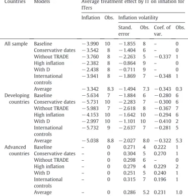
Table 6

Aggregate results.

Countries Models Average treatment effect by IT on inﬂation for ITers

Inﬂation Obs. Inﬂation volatility Stand.

error Obs. Coef. ofvar. Obs. All sample Baseline −3.990 10 −1.855 8 – 0

Conservative dates −3.542 8 −1.404 6 – 0 Without TRADE −3.760 8 −2.263 5 −0.337 1 High inﬂation −2.382 8 −0.864 9 – 0 With D −2.438 8 −0.711 9 – 0 International

controls

−3.941 8 −1.869 7 −0.348 1

Average −3.342 8.3 −1.494 7.3 −0.343 0.3 Developing

countries

Baseline −5.634 7 −1.884 6 −0.280 6 Conservative dates −5.731 10 −2.283 7 −0.300 6 Without TRADE −5.983 7 −2.618 8 −0.367 7 High inﬂation −4.153 10 −1.642 10 −0.294 6 With D −2.997 10 −1.101 10 −0.410 2 International

controls

−5.732 9 −2.637 7 −0.281 5

Average −5.038 8.8 −2.027 8.0 −0.322 5.3 Advanced

countries

Baseline – 0 0.271 4 0.222 1 Conservative dates – 0 0.304 5 0.270 1 Without TRADE – 0 0.298 6 – 0 High inﬂation – 0 0.279 4 0.229 2 With D – 0 0.251 5 0.240 1 International

controls

– 0 0.315 7 0.196 1

Average – 0 0.286 5.2 0.231 1.0 Note: Only statistically signiﬁcant results. Obs.: number of signiﬁcant results (10%).

27_{This presentation takes into account} _{Rosenbaum and Rubin (1983), Imbens}

(2000), and Becker and Ichino (2002). 28_{In this case the Probit model was chosen.}